Article

Prediction of Battery Electric Vehicle Energy Consumption via Pre-Trained Model Under Inconsistent Feature Spaces

School of Ocean and Civil Engineering, Shanghai Jiao Tong University, Shanghai 200240, China
*
Authors to whom correspondence should be addressed.
Technologies 2025, 13(11), 493; https://doi.org/10.3390/technologies13110493
Submission received: 15 September 2025 / Revised: 14 October 2025 / Accepted: 27 October 2025 / Published: 29 October 2025
(This article belongs to the Topic Dynamics, Control and Simulation of Electric Vehicles)

Abstract

Accurately predicting the trip-level energy consumption of battery electric vehicles (BEVs) can alleviate range anxiety of drivers and improve intelligent route planning. However, although data-driven methods excel in predicting with multi-feature inputs, each vehicle often requires a dedicated model due to potential inconsistencies in feature spaces of collected data. Consequently, the necessity of sufficient trip data challenges newly registered vehicles. To address the challenges, this study proposed a transformer-based pre-trained model for BEV energy consumption prediction adapting to inconsistent feature spaces, referred to as IFS-Former. By innovatively introducing trainable missing-feature embeddings and placeholder masks, the IFS-Former can tolerate new or missing features of downstream tasks after pre-training. The IFS-Former was pre-trained on a dataset comprising 837 vehicles from 8 different cities, containing 492 thousand trips, and validated on 13 vehicles with inconsistent feature spaces. After applying transfer learning to the 13 vehicles, the pre-trained IFS-Former attains high prediction accuracy (R2 = 0.97, mean absolute error (MAE) = 1.19). Even under extremely inconsistent feature spaces, the IFS-Former maintains robust performance (R2 = 0.96, MAE = 1.31) leveraging its pre-trained knowledge. Furthermore, the IFS-Former is well-suited for on-board deployment with a size of only 32 MB. This study facilitates on-board artificial intelligence for accurate and practical energy consumption prediction.

1. Introduction

As a new generation of environmentally friendly transportation, electric vehicles (EVs) represent a significant milestone in the ongoing electrification of the automotive industry. The merits of these EVs are manifold, including high energy efficiency, low noise, intelligence, and reduced pollutant emissions, and their ownership is growing rapidly [1,2,3]. Battery electric vehicles (BEVs) are fully powered by their batteries. This makes them much more environmentally friendly and convenient, and they account for a significant proportion of EVs [4,5]. This study focuses on the trip-level energy consumption prediction of BEVs. In comparison with the refuelling process of conventional internal combustion engine vehicles, the charging process of BEVs is more time-consuming, and the energy consumption is more susceptible to changes caused by various factors such as environmental temperature [6]. Consequently, drivers are often concerned with the question of how far can the BEV still travel, a phenomenon referred to as range anxiety [7]. Accurately predicting the trip energy consumption can enhance the accuracy of remaining range prediction and mitigate the range anxiety experienced by drivers [8].
In recent times, the trip energy consumption prediction of BEVs usually adopts the historical energy consumption rate method, which directly predicts energy consumption based on information from the previous trips [9]. This approach is eminently practical, yet it fails to take into account the heterogeneity of each trip. It fails to consider the influence of driving behaviour, meteorological conditions, and traffic status, resulting in limited prediction accuracy [10]. With the advancement of artificial intelligence (AI), data-driven prediction models have demonstrated more accurate prediction capabilities [11]. Building on this progress, researchers have constructed features of factors influencing energy consumption based on field data and performed energy consumption prediction using quantile regression forests [12]. Additionally, artificial neural networks were applied to predict BEV energy consumption with detailed feature selection [13]. Furthermore, deep neural networks were adopted to predict BEV energy consumption by combining static and dynamic data relating to specified routes [14]. In further efforts, researchers compared multiple machine learning models, including multiple linear regression (MLR), extreme gradient boosting (XGBoost) [15], and support vector regression (SVR) [16] for BEV energy consumption prediction, finding that XGBoost achieved higher accuracy and providing interpretability analysis of the model outputs [17]. Ref. [18] employed a combination of random forest and gradient boosting decision tree models with a view to constructing a more reliable energy consumption prediction model. Ref. [19] employed sequence modelling on the trips and utilised deep learning methods, including long short-term memory (LSTM) and temporal convolutional networks, to predict energy consumption. Concurrently, with the emergence of the Transformer [20], more advanced models such as TabTransformer have been applied for BEV energy consumption prediction [21]. Ref. [22] proposed an integrated model combining LSTM and Transformer architectures, which significantly enhances the predictive accuracy of BEV energy consumption.
However, most existing data-driven methodologies presuppose that the input features are immutable [23,24], a premise that renders them incapable of modification once the model has been trained. In practice, due to differences in on-board sensors, data acquisition systems and data privacy agreement across different vehicle models, the collected features are often not the same [25,26]. For instance, some datasets may lack records of accelerator and brake pedal positions, which are deemed to be critical for characterising driving behaviour [25]. It is important to note that, even for the same vehicle, some features may be missing during different trips. This can be attributed to data transmission errors or sensor failures [27,28]. Furthermore, in real-world scenarios, in order to adequately account for heterogeneities in driving behaviour and state-of-health (SOH) of the batteries, it is necessary to train a dedicated model for each vehicle [22,29]. However, for a newly registered vehicle, it may take a significant amount of time may be required to accumulate sufficient trip data to train a high-performing prediction model [23].
In scenarios where the downstream task data are scarce, the merits of pre-training and transfer learning become evident. Pre-training is a process whereby a model is initially trained on large-scale datasets to capture general knowledge. A pre-trained model learns general representations from the source domain and can efficiently adapt to data-scarce environments through transfer learning (training quickly within limited epochs) on the downstream tasks, achieving excellent performance. This capability has been extensively validated in the fields of natural language processing (NLP) and computer vision (CV) [30,31]. In the domain of BEVs, relevant studies have also confirmed the feasibility of pre-training and transfer learning. For example, Ref. [32] pre-trained a machine learning model for trip energy consumption prediction on a large dataset from a BEV model and subsequently transferred it to another new BEV model with only a small amount of trip data. This approach led to a significant reduction in prediction error. Building upon this concept, a Transformer-based pre-trained model for energy consumption prediction was proposed using a large collection of trip data from BEVs, which could be quickly adapted to downstream vehicles through transfer learning, thus addressing the issue of limited data for newly registered vehicles [23]. In a similar vein, another energy consumption prediction model for BEVs was proposed and achieved energy consumption prediction across different vehicle models through few-shot learning [33].
Currently, studies are underway on the utilisation of pre-trained models for predicting energy consumption of BEVs. While some studies have already considered data scarcity in downstream tasks [23,32], they have not yet taken into account changes in feature spaces. In general, feature changes are not drastic for BEV trip energy consumption prediction tasks. If the model can learn much as possible about the representation of different features during pre-training, the knowledge acquired can still be useful when some changes in features occur.
This study specifically targets scenarios where both data scarcity and feature space changes exist. The Transformer architecture is selected to construct the model for its flexibility and efficient computational performance [20]. It has demonstrated outstanding performance in NLP and CV tasks [34,35,36], and has also shown strong potential in regression tasks [37,38,39,40]. A Transformer-based pre-trained model adapting to inputs with inconsistent feature spaces is proposed to achieve trip energy consumption prediction for BEVs under different feature spaces, referred to as IFS-Former. The research methodology for this study is illustrated in Figure 1. Trip information and corresponding features are extracted from real-world data and fed into the IFS-Former for pre-training. The IFS-Former activates sufficient feature spaces, extracting as many features as possible during pre-training while masking placeholder features. During training, missing features are constructed as trainable embeddings, enabling the IFS-Former to adapt to feature missing. In downstream prediction tasks, through a flexible combination of missing feature padding and placeholder feature masking, together with transfer learning, the IFS-Former can accommodate to reduced or newly added features with scarce samples of downstream tasks. The subsequent sections of this paper will provide a more detailed discussion of the data feature engineering and model training procedures employed in this study. The main contributions of this study are listed as follows:
  • A universal model for BEV trip energy consumption prediction, the IFS-Former, was developed and trained, achieving higher accuracy than vehicle-specific models.
  • Feature missing was introduced in large-scale datasets during pre-training to enable the IFS-Former to adapt to inconsistent vehicle feature spaces.
  • The robust strength of the IFS-Former under extremely inconsistent feature spaces was demonstrated through feature ablation experiments.
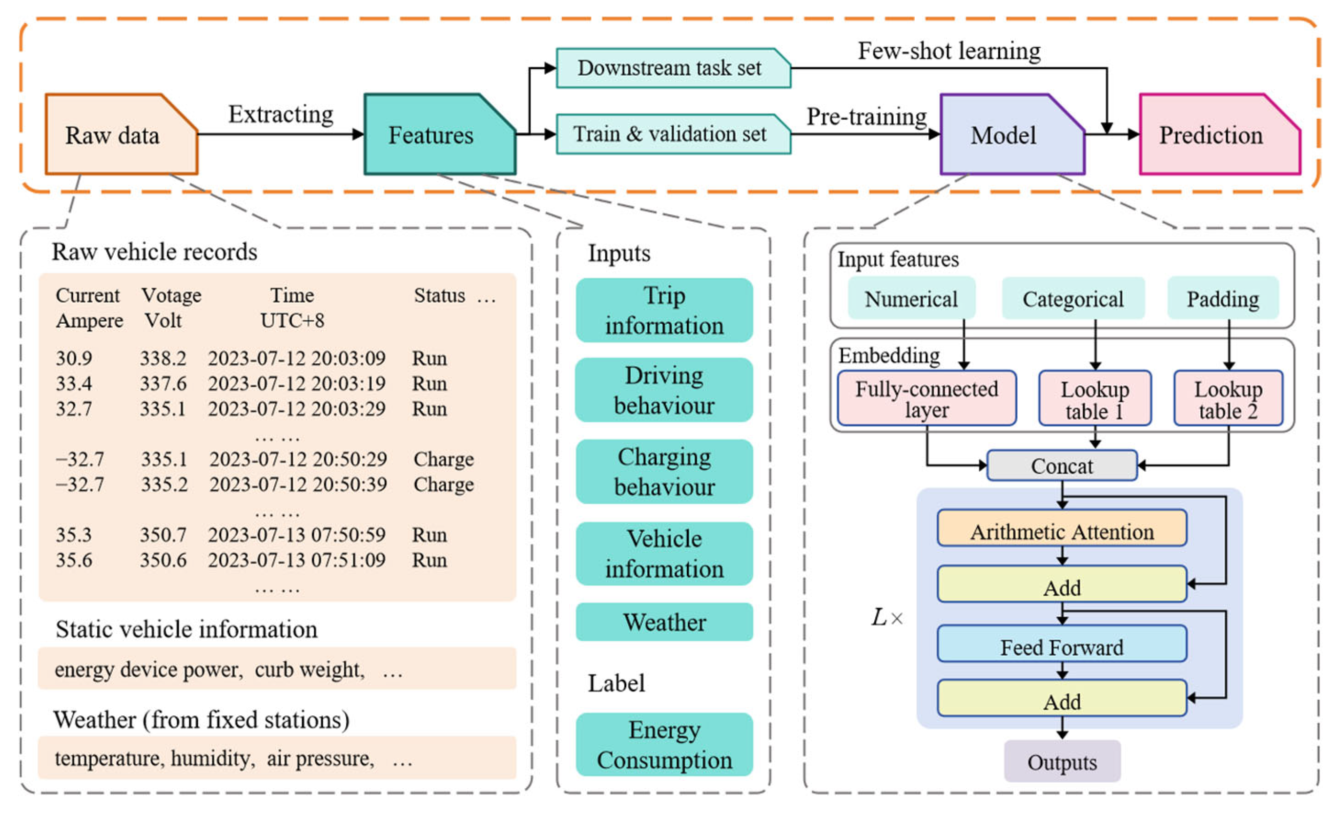
Figure 1. The flowchart of this study.
Technologies 13 00493 g001

2. Scenarios and Data

2.1. Data Description and Pre-Processing

This study utilises real-time operational data collected from 850 BEVs, sourced from the National Big Data Alliance of New Energy Vehicles Open Lab, and the Shanghai Electric Vehicle Public Data Collecting, Monitoring and Research Center. The data collection methodology conforms to the specifications outlined in the National Standard of China: GB/T 32960-2016, Technical specifications for remote service and management system for electric vehicles [41]. The data were sampled at a standard frequency of 0.1 hertz (Hz), including timestamps, vehicle status, voltage, current, and other real-time information. The temporal and geographical scope of the dataset extends from December 2020 to May 2024, covering 20 different vehicle models distributed across 8 Chinese cities (Tianjin, Guangzhou, Leshan, Dongguan, Shenzhen, Chengdu, Beihai and Shanghai). The dataset currently contains more than 500 million records. In addition, the maximum power, maximum torque, curb weight, and wheelbase of the vehicle were obtained from the official announcement.
It is evident that the processes of collecting, transmitting, and storing BEV data are inherently complex. Consequently, the dataset inevitably contains duplicate values, outliers, and missing values. Duplicate values were deleted directly. Outliers in the original data, typically resulting from errors in the data collection process, were automatically identified by the transmission system and removed based on a predefined rule table. Missing values were attributed to discontinuities in the temporal data stream, and so were not imputed, since vehicle operating conditions are subject to change in real time, and imputation could potentially result in errors. In instances where missing values impeded feature extraction, the IFS-Former demonstrated its capacity to handle such scenarios in this study.
To investigate the impact of temperature and other factors on BEV energy consumption, meteorological data were obtained from the website https://rp5.ru (accessed on 19 May 2025). The meteorological dataset was collected from meteorological stations in different cities at 1 or 3 hourly intervals., while also inevitably containing a limited number of missing values. In response to these factors, the meteorological data was addressed through linear imputation, with hourly standard timestamps serving as a reference point.
All the original data mentioned above are comprehensively demonstrated with illustrative examples in Table 1.

2.2. Trip Extraction

This study aims to develop a trip energy consumption prediction model that can predict the energy consumption of an individual trip directly from input features. However, as shown in Figure 1, the original vehicle data merely records the instantaneous state of vehicles at fixed time intervals and cannot be utilised directly for model training. The initial step involves the extraction of each trip from the original data. Subsequently, the construction of other features associated with that trip is necessary, and these are then fed into the model for training.
Within the original vehicle data (Table 1), driving records can be systematically identified through the vehicle status field, which indicates the vehicle is running. The delineation of trip boundaries was achieved by implementing a temporal threshold of 3 min. If the time interval between 2 consecutive driving records exceeded this threshold, the onset of a new trip was assumed. It is noteworthy that adopting a longer threshold would allow for a greater tolerance of missing data. Nevertheless, this adjustment may undermine the accuracy of trip-level energy consumption prediction.

2.3. Feature Construction

In this study, the target variable is trip energy consumption. According to previous studies [6,23], the trip energy consumption can be extracted based on the trip segments, which is calculated using the following formula:
T E C = i = 1 s 1 V i × I i 1000 × t i 3600 ,
where T E C is the trip energy consumption, s denotes the length of the trip segment. V i and I i represent the voltage in volt and current in ampere at each time step, respectively. t i refers to the time interval in second between the current timestamp and the next one. The calculated result is expressed in kilowatt hour (kWh).
In order to enhance the accuracy and reliability of BEV trip energy consumption prediction, it is necessary to identify and extract a multitude of factors that exert influence on trip energy usage. From the perspective of trip-level analysis, the trip distance is directly proportional to energy consumption [6]. It can thus be concluded that a basic method for predicting trip energy consumption is to multiply the historical mean energy consumption rate by the distance of the current trip. However, this method is limited in accuracy, as numerous other factors also significantly influence trip energy consumption [42]. In terms of driving behaviour, aggressive driving behaviour leads to higher energy consumption [43]. From the perspective of battery status, variations in the state-of-charge (SOC) can alter the output efficiency of the battery, thereby influencing energy consumption [44]. The SOH of the battery can be reflected by changes in internal resistance [45], which also influences output efficiency and ultimately impacts trip energy consumption. With regard to the characteristics of vehicles, it is evident that different vehicle models vary in parameters such as wheelbase, power, and curb weight. These factors have the capacity to influence energy consumption. From the meteorological standpoint, under low-temperature conditions, batteries require additional energy for preheating [46]. Furthermore, under conditions of extremely high temperature, there is also an increase in BEV energy consumption [47]. In addition, wind speed exerts a notable influence on BEV energy consumption [48]. In relation to traffic conditions, traffic states directly influence driver behaviour (e.g., long periods of idling or low-speed driving), which in turn influences the efficiency of the drive motor and ultimately impacts energy consumption [49]. The built environment also impacts energy consumption (e.g., road slopes [50]).
The data obtained in this study was used to construct 6 categories of features, namely trip information, driving behaviour, charging behaviour, vehicle information, weather, and transportation. The built environment like road slopes were not considered due to the de-identification of most of the original and the absence of GPS information.
Initially, trip information features were extracted. When predicting energy consumption using trip distance, the considered features included trip distance, historical energy consumption rate, and the current time. In this study, random noise within ±5% was added to all extracted trip distances. This was due to the fact that the trip distance, when predicting future trip energy consumption, is dependent on prediction provided by the on-board navigation system, which is typically unable to perfectly predict the actual travel distance. This helps to prevent the IFS-Former from over-relying on trip distance, thereby improving its robustness.
Subsequently, driving behaviour and charging behaviour features were constructed. Driving behaviour was primarily characterised using accelerator pedal and brake pedal records, while charging behaviour was represented mainly by the charging patterns of users. Most of these features were directly extracted from the original data. Special attention should be given to the definition of the energy recovery ratio, which is defined as follows:
E R R = i = 1 s 1 V i × R e L U ( I i ) × t i / ( 1000 × 3600 ) i = 1 s 1 V i × R e L U ( I i ) × t i / ( 1000 × 3600 ) ,
where E R R is the energy recovery ratio, V i is always non-negative, and I i is positive when representing energy output and negative when representing energy recovery. The numerator of this equation represents the total energy recovered, while the denominator denotes the total energy output (in kWh). Their ratio is the energy recovery ratio.
After extracting the 3 categories mentioned above, vehicle information and weather were appended directly. This process completed the initial construction of the 5 major feature categories (Figure 2).
Despite the preliminary processing of the original data, abnormal trips still needed to be removed after the initial construction. Specifically, trips were excluded if they met any of the following criteria: trip duration less than 10 min [51], trip distance less than 1 km, mean trip speed less than 1 km/h, total trip energy consumption less than 0.1 kWh, initial SOC less than 5% [23]. For other continuous features, any values deviating by more than 3 times standard deviations from the mean values were treated as outliers, and the corresponding trip records were removed.
Furthermore, to account for potential increases in available features during downstream tasks, an additional transportation feature category was designed to represent the overall traffic conditions experienced by the vehicle during a trip. This category comprised 2 features: trip time and trip mean speed. However, given that obtaining future traffic conditions depends on highly accurate predictions through on-board navigation systems, a relatively challenging feat, the 2 features of transportation were extracted solely for the purpose of downstream prediction tasks and were not added during the pre-training process.
A total of 506,138 trip records from 850 vehicles were obtained. The complete data from 13 randomly selected vehicles (13,304 trips) were kept for downstream prediction tasks. The remaining data from the left 837 vehicles (492,834 trips) were used for pre-training. The features and their relationships with energy consumption are shown in Figure 2. There are a total of 6 categories and 50 features. Among them, the 2 features of transportation were only extracted from 2 vehicles of the downstream prediction tasks, so the points of these 2 features appear relatively scarce. It can be observed that there exists a relatively direct linear relationship between trip distance, trip time, and trip energy consumption. Meanwhile, a relatively direct linear relationship is evident between the remaining SOC and the maximum trip energy consumption. The impact of additional features on trip energy consumption may only become evident through their interactions with features such as trip distance and trip time. This underscores the necessity for trip energy consumption prediction models to incorporate feature interactions.

3. Methodologies

3.1. The Transformer Architecture for Inconsistent Feature Spaces

The Transformer architecture is selected for the construction of the prediction model due to its efficient computation and architectural flexibility. Given that trip energy consumption is directly related to trip distance, and the influences of other features are often mediated through distance, the arithmetical feature interaction-based Transformer (AMFormer) [39] is employed as the backbone network.
At the input layer, all features are classified into categorical features ( x c a t e ) and numerical features ( x n u m e ). Categorical feature embeddings are obtained via a process of table look-up, while numerical feature embeddings are obtained through the application of linear transformation.
This study addresses the potential occurrence of feature missing or feature addition in BEV data collection by adopting a token-truncation strategy inspired by NLP models. A maximum input feature length is predefined, and each feature position is associated with a trainable embedding representing a missing feature. The embedding is stored in a lookup table in the same manner as categorical feature embeddings (Figure 1). During the pre-training stage, only a subset of feature positions is activated, with actual feature values fed into these positions. In instances where a feature value is missing in a specific position, the corresponding trainable missing-feature embedding is utilised for padding. The embeddings participate in training and parameter updates, thereby enabling explicit modelling of missing information. Positions representing features that are only for placeholder are masked [20] like the padding tokens in an NLP model, and their embeddings remain in the initialised state to prevent them from contributing to the final output. Then the embeddings ( e c a t e   /   n u m e ) are formulated as
e j c a t e / n u m e = e j c a t e = C e m b e d [ x j c a t e ] , j a c t i v e ,   x j   o b s e r v e d e j n u m e = x j n u m e w j + b j , j a c t i v e ,   x j   o b s e r v e d M e m b e d [ j ] , j ( a c t i v e ,   x j   m i s s i n g ) p l a c e h o l d e r ,
where C e m b e d is the embedding table of categorical features, M e m b e d is the embedding table of missing features, and w j ,   b j R d are trainable parameters. The input tensor is obtained through concatenating the embeddings of categories and numerical features:
X = [ e j c a t e ] j = 1 l e n ( c a t e ) [ e j n u m e ] j = l e n ( c a t e ) + 1 l e n ( c a t e ) + l e n ( n u m e ) R N × d ,
where X represents the input embeddings, denotes the concatenation of the categorical and numerical feature embeddings along the feature dimension.
After pre-processing the input, the feature interaction stage follows the core mechanism of the AMFormer, which models the relationships between different features using a combination of additive attention and multiplicative attention. AMformer does not require explicit modelling of feature interactions. Instead, it accomplishes this through attention mechanisms. This approach facilitates the streamlining of the input features, and also enabling the capture of feature interactions that enhance the performance of the final prediction. Let the input embeddings be X R N × d . The additive interaction is implemented directly via a multi-head attention mechanism, where Q a d d = X W Q a d d , K a d d = X W K a d d , V a d d = X W V a d d , W Q a d d , K a d d , V a d d R d × d . The additive interaction attention is formulated as
A t t e n t i o n A = s o f t m a x Q a d d K a d d T d V a d d R N × d ,
For multiplicative interactions, the input feature embeddings are transformed using a logarithmic function, then the multiplicative interaction is computed:
X log = log ( ReLU ( X ) + ϵ ) R N × d ,
A t t e n t i o n M = exp s o f t m a x Q l o g K l o g T d V l o g R N × d ,
where ϵ is a small positive constant used to avoid taking the logarithm of 0. The additive interaction and multiplicative interaction are then combined and passed through a fully connected layer that decreases the dimension.
The functionality of feature interaction enables the IFS-Former to capture the combined influences of trip distance and other features on the energy consumption. By combining missing-feature padding and masking strategies, the IFS-Former has the capability to accommodate any input feature set whose size does not exceed the predefined maximum length. This enhancement to its robustness to feature addition or missing is significant.

3.2. The Loss Function

In this study, the distribution of trip distances was found to be imbalanced, with long-distance trips being relatively scarce. However, range anxiety is more pronounced during long-distance trips. To improve the prediction accuracy of the IFS-Former for long-distance trip energy consumption, a weighted loss function based on mean square error (MSE) was adopted, which is a commonly used approach in the field of imbalanced data [52]. According to previous studies [43,53], trips were categorised into 3 groups by distance (Table 2). In this study, an inverse-proportional weighting strategy based on the sample size of each group was applied to balance the influence of different trip distances in training. The formula of weighting is as follows:
w e i g h t q = n k × g q ,
where w e i g h t q denotes the weight of a sample, n represents the total number of samples, k indicates the number of groups, and g q refers to the number of samples in the group. The sample counts and the corresponding weights calculated through the equation are presented in Table 2.

3.3. Settings for Numerical Experiments

3.3.1. Pre-Training and Transfer Learning

In this study, the embedding dimension was set to 256, and the Transformer architecture consisted of 8 attention heads and 6 encoder layers, with each feed-forward network having a dimension of 1024. The batch size for training was fixed at 64. In order to accelerate convergence, an active learning rate adjustment strategy was employed, utilising a cosine annealing schedule with restarts. The initial maximum learning rate was 1.5 × 10⁻⁵, the minimum learning rate was 1 × 10⁻⁷, and each cosine annealing cycle lasted 25 epochs, after which the maximum learning rate was reduced to 70% of its previous value. The continuous features were normalised using min-max scaling prior to being fed into the IFS-Former. During the period of pre-training, 10% of the training dataset was randomly sampled as a validation set to monitor convergence in real time.
To simulate the issue of missing features in downstream tasks, artificial feature missing was introduced into the training data. In most cases, the original vehicle data supports extraction of most features. However, in some cases, there is a missing of data of accelerator and brake pedal records, which hinders the extraction of driving behaviour. In other cases, downstream datasets may lack detailed battery records, resulting in incomplete charging features. Consequently, only the complete missing of major feature categories were considered, including driving behaviour, charging behaviour, vehicle information and weather. Trip information was considered indispensable in this study. The missing proportion for each category was set to be 20%.
For pre-training, a total of 48 features were used, encompassing 5 categorical features and 43 continuous features. The maximum input sequence length was designated as to 96 (24 categorical features and 72 continuous features), thus permitting the incorporation of supplementary features in downstream tasks.
In downstream transfer learning, 5 different sample sizes were used for each vehicle: 32, 64, 128, 256, and 384. To avoid data leakage, the training was performed only on the first 384 samples in chronological order and testing was conducted exclusively on samples from the 385th onward. This transfer learning setting, where the pre-trained model is fine-tuned with a small number of labelled samples, can be regarded as few-shot learning. For completeness, the pre-trained model without fine-tuning was also considered, which is defined called zero-shot. The batch size for few-shot learning was set to 32 in order to accommodate small-sample scenarios. To prevent catastrophic forgetting of pre-trained knowledge, few-shot learning was limited to 10 epochs following a cosine-annealing two-stage learning rate schedule. In epoch 1 to 5, the backbone network were frozen, only the embeddings were optimised, with an initial learning rate of 5 × 10⁻⁶. In epoch 6 to 10, the backbone network was unfrozen, and joint few-shot learning of both backbone and embeddings was performed. The initial learning rates for both were set to 5 × 10⁻⁷, and annealed towards 0 using cosine decay.

3.3.2. Baseline Models

For comparison, several BEV trip energy consumption prediction methods are selected as baseline models, including multiplying the historical energy consumption rate by the predicted trip distance (ECR × d) [23], MLR [17], the XGBoost [17], the light gradient boosting machine (LightBGM) [24] and the Markov-based Gaussian processing regression (M-GPR) [54]. Each of these models was independently trained and tested on the dataset of each individual vehicle of downstream tasks. All numerical experiments were conducted on a Linux server equipped with an Intel Core i9-7940X CPU and 2 NVIDIA TITAN RTX GPUs. All the programme was run in a Python 3.10 environment.

3.3.3. Evaluation Metrics

Coefficient of determination (R2), Bias, mean absolute error (MAE), root mean square error (RMSE) and mean absolute percentage error (MAPE) are selected as evaluation metrics, which are commonly used in regression tasks [55]:
R 2 = 1 q = 1 n ( y q y ^ q ) 2 q = 1 n ( y q y ¯ ) 2 ,
B i a s = 1 n q = 1 n ( y ^ q y q ) ,
M A E = 1 n q = 1 n | y q y ^ q | ,
R M S E = 1 n q = 1 n y q y ^ q 2 ,
M A P E = 100 % n q = 1 n | y q y ^ q y q | ,
where y q denotes the true values of the samples, y ¯  represents the mean value of the samples, and y ^ q  indicates the prediction values of the samples.

4. Results and Discussion

4.1. Accuracy of Downstream Tasks

The proposed IFS-Former contains over 8 million trainable parameters. Pre-training was conducted for approximately 30 h, over 150 epochs (1,039,650 steps). During training, the loss on both the training and validation sets decreased gradually and eventually converged, completing the pre-training stage.
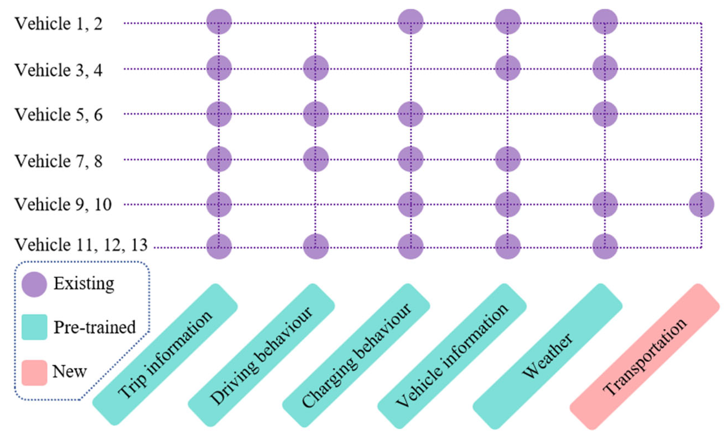
The downstream tasks were performed using operational data from 13 independent vehicles. These vehicles represent several inconsistent feature spaces compared to the pre-trained feature spaces (Figure 3). For example, Vehicle 1 and 2 lack of driving behaviour, and Vehicle 9 and 10 also lack driving behaviour, although they have transportation features.
The predictive metrics of different models on downstream tasks are presented in Table 3 and Figure 4. In Table 3, The missing results indicates R2 < 0.6, the ± denotes the standard deviation and the p-values for all methods tested on each individual vehicle are much less than 0.001. The findings indicate that the IFS-Former attains optimal performance, signifying robust transferability following large-scale pre-training. In the zero-shot setting, the IFS-Former attains high prediction accuracy (R2 = 0.97, Bias = −0.07, MAE = 1.19, RMSE = 1.76, MAPE = 0.13). This suggests that the pre-training process provides the IFS-Former with sufficient knowledge, thereby enabling effective generalisation to vehicles it has never encountered. In addition, under the few-shot learning, the IFS-Former maintains stable performance and consistently outperforms all baseline models. At the 384-shot setting, compared with the IFS-Former, the R2 of the baseline models decrease by 1.57% to 15.89%, while their MAE increase by 18.62% to 157.47%. While the IFS-Former shows continuous improvement, with a decline in Bias of 15.42% at the 384-shot setting in comparison to the zero-shot setting. This phenomenon indicates that the IFS-Former becomes more adaptable to each individual vehicle after few-shot learning, reducing the possibility of overestimating or underestimating the trip energy consumption.
In comparison, traditional tree-based methods (XGBoost and LightGBM) exhibit a more pronounced performance improvement as the number of samples increases. The R2 of the XGBoost improves from 0.80 in the 32-shot learning setting to 0.93 in the 384-shot learning setting. For the LightGBM, the R2 increases from 0.85 in the 128-shot learning setting to 0.93 in the 384-shot learning setting. This indicates that these models possess strong fitting capabilities when data are sufficient. However, collecting 384 samples in practical vehicle usage scenarios requires a considerable amount of time, especially for daily commuting usage, where obtaining from the start of vehicle ownership may take a long period. Therefore, considering data efficiency and practical applicability, the IFS-Former offers greater advantages in general scenarios.
The traditional ECR × d method achieves relatively stable performance, with an R2 of 0.95. However, the IFS-Former yields a better performance (in the 384-shot setting, the MAE of ECR × d is 18.62% higher), indicating the IFS-Former produces higher accuracy for individual trip-level predictions.
For the M-GPR and the MLR, the performance is comparatively poor. At the 384-shot setting, the R2 of the M-GPR remains at only 0.81, with the MAE reaching 3.07, which falls short of accuracy requirements. Compared to other models, the M-GPR exhibits the greatest negative Bias, indicating that it tends to underestimate energy consumption. This renders it unsuitable for practical applications. This may be due to the limited ability of such models to capture complex nonlinear relationships and their inadequate generalisation in multiple feature spaces. In the case of the MLR, the model lacks a unique solution when the number of samples is smaller than the number of features. Even when the sample size slightly exceeds the number of features, it still suffers from unstable parameter estimation and insufficient convergence, thereby resulting in suboptimal predictive performance.
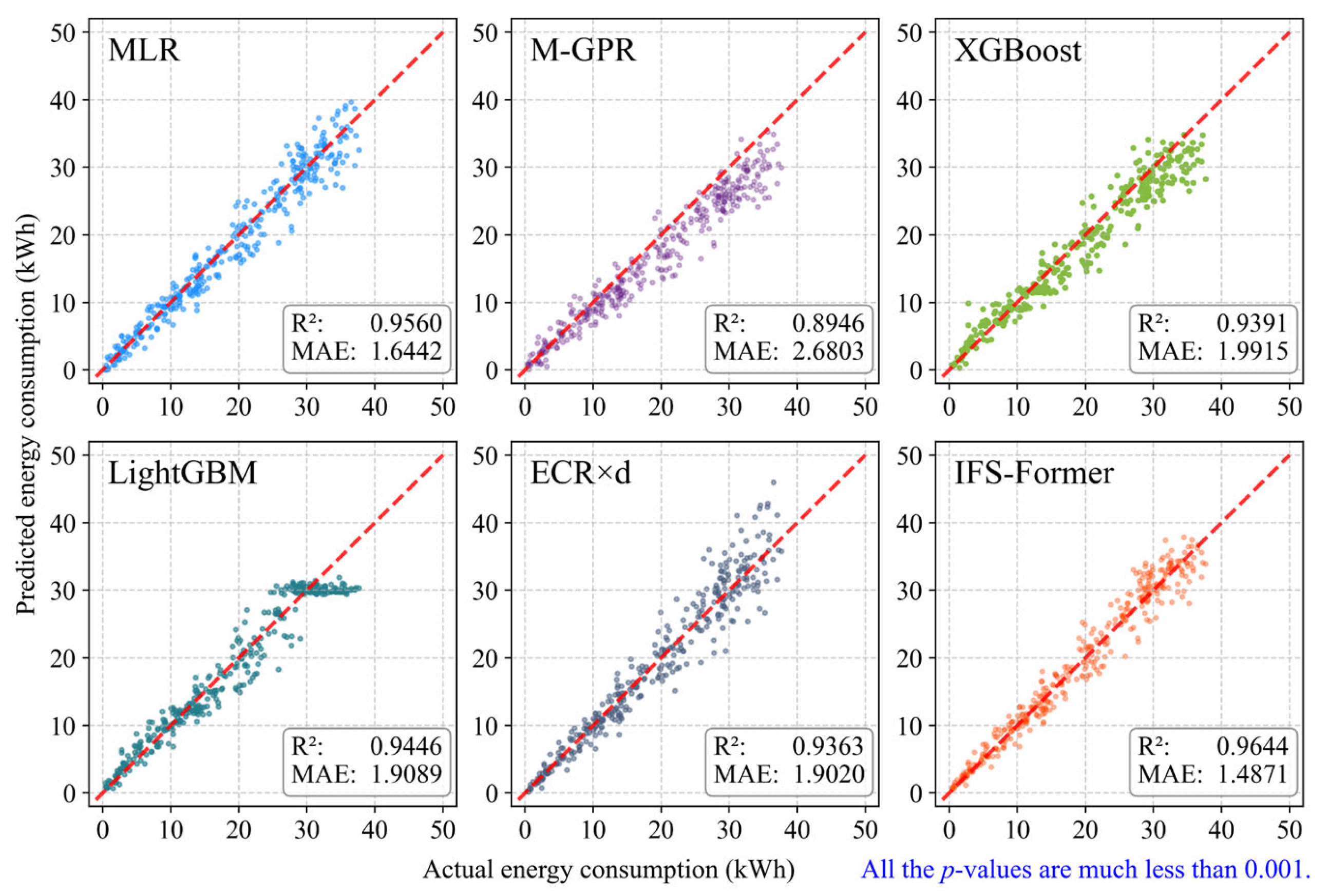
In the 384-shot setting, a vehicle is randomly selected for visualisation (Figure 5). As can be seen, the IFS-Former achieves the best overall performance, with the R2 of the baseline models reducing by 0.87% to 7.23% and the MAE increasing by 10.56% to 80.23% in comparison. The ECR × d method exhibits increasing prediction errors for long-distance trips. Although the MLR model performed relatively well on this vehicle, its overall performance (Table 3) indicates that its training remains somewhat unstable at the current sample size. The LightGBM and the XGBoost may not have reached their full potential under this sample size. The M-GPR consistently predicts the energy consumption lower than the actual values for most trips, which is highly undesirable in practical energy consumption prediction scenarios, as such prediction could mislead drivers and should therefore be avoided.

4.2. Ablation Analysis of Features

In order to evaluate the robustness of the IFS-Former under different feature-missing scenarios, an ablation study was conducted. The study used the 13 vehicles of downstream tasks on the 4 feature categories included: driving behaviour, charging behaviour, vehicle information, and weather (trip information is handled as an indispensable feature category). The following four feature groups were added to the missing state in sequence, based on the original test set. If a vehicle did not originally contain a given feature, it was kept missing throughout the process. The results of ablation analysis are demonstrated in Figure 6.
As shown in Figure 6, the performance of the IFS-Former exhibits a gradual decline as the number of available features diminishes. When only the trip information is retained, the results of the 384-shot setting indicate that the R2 decreases by 0.62% and the MAE increases by 9.91% compared to the scenario with the original features. This ablation result, however, validates the necessity of selecting multiple feature categories as inputs for maintaining model performance.
Despite the decline in the performance of the IFS-Former declines when certain downstream features are missing, it continues to demonstrate commendable performance (R2 = 0.96, MAE = 1.31), surpassing the performance of all baseline models with original feature spaces. This superiority can be attributed to the construction of missing features during pre-trainging, enabling the IFS-Former to learn representations of missing features. Consequently, even when a given feature is missing, the IFS-Former is capable of constructing the embeddings for the missing information based on pre-trained knowledge, thereby ensuring the maintenance of strong performance in scenarios where a high proportion of features are missing.

4.3. Efficiency and Interpretability of the Model

The parameters of the IFS-Former are stored in a 32 MB pth file in Float32 single-precision floating-point format, facilitating on-board deployment on vehicle terminal devices thanks to its lightweight design. Experimental results show that in the few-shot learning settings, the IFS-Former achieves training and inferencing speed of 1.7 and 0.8 ms/sample, which are comparable to those of other models in the same category [23]. Its high computational efficiency satisfies the requirement for real-time energy consumption prediction before departure, enhancing the feasibility of deploying the IFS-Former on-board.
Recently, the reliability of deep learning models is attracting increasing attention, with interpretability being a key evaluation indicator. For Transformer-based architectures, previous studies have shown that relying solely on attention distributions can reflect the interactions between features, but may not necessarily be closely related to the final outputs [56]. In contrast, incorporating gradient information helps reveal the sensitivity of model outputs to input features [57]. In this study, a method based on the fusion of attention and gradient information is employed to interpret the prediction process of the IFS-Former on tabular data. Attention weights are used to capture structural relationships among features. Gradient signals are introduced to emphasise those connections with higher impact on the prediction target. Subsequently, weighted aggregation is performed across multiple heads and layers, combined with residual correction and gating mechanisms, to derive the integrated contribution of each feature to the final prediction. Compared to relying solely on attention or gradient information, the proposed method provides a more stable and intuitive depiction of feature importance, effectively highlighting key features in model decision-making and offering stronger interpretability support.
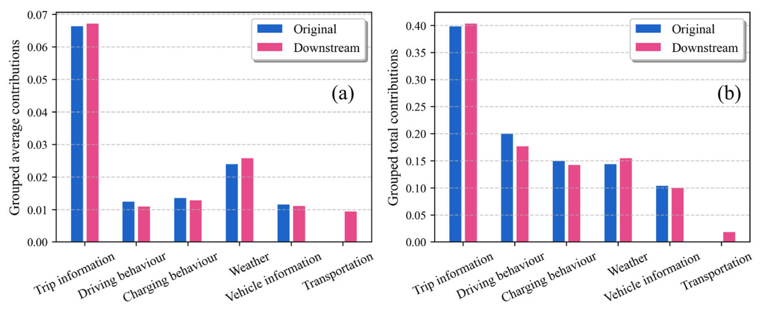
Under the 384-shot setting, model interpretability was computed using the pre-trained IFS-Former in two scenarios: Scenario 1 is the original feature spaces consistent with pre-training (Vehicle 9 and 10), while Scenario 2 is feature spaces with no driving behaviour but with transportation features (Vehicle 11, 12 and 13). Figure 7 shows the mean and overall contributions of each feature group. The results reveal that trip information makes the largest contribution to the prediction task. Weather also significantly influences trip energy consumption, likely due to variations in on-board air conditioning usage under different weather conditions. Transportation features were missing in Scenario 1 but present in Scenario 2 and were still able to contribute to predictions after few-shot learning. Driving behaviour features were present in Scenario 1 but missing in Scenario 2, thus their contribution decreased. However, interpreting deep learning models remains challenging, and the actual reduction in contribution due to missing driving behaviour may be greater than that reflected in the figure.

5. Conclusions

In this study, a pre-trained model, designated IFS-Former, was proposed for the prediction of BEV trip-level energy consumption. The model was developed to adapt to downstream inconsistent feature spaces and data scarcity. The IFS-Former was pre-trained with large-scale trip data extracted from real-world driving records of numerous BEVs and was subsequently evaluated through zero-shot and few-shot tests on downstream BEVs with inconsistent feature spaces to verify its accuracy and generalisation capability. In addition, the robustness of the IFS-Former under reduced feature spaces was examined through the ablation analysis. The primary conclusions that can be drawn from this study are as follows:
  • The proposed pre-trained IFS-Former model demonstrates superior performance over baseline models in BEV energy consumption prediction. After extensive pre-training, the IFS-Former achieves high accuracy on downstream tasks even without few-short learning (zero-shot, R2 = 0.97, Bias = −0.07, MAE = 1.19), and its performance further improves with few-shot learning (384-shot, Bias decreasing by 15.42%), and the MAE of the baseline models increases by 18.62% to 157.47% compared to the IFS-Former under the same setting.
  • Large-scale pre-training is leveraged to address inconsistent feature spaces in downstream tasks. Trainable missing-feature embeddings are introduced to enable the IFS-Former to handle feature missing scenarios. Moreover, artificially induced feature missing is incorporated into the pre-training data to help the IFS-Former learn effective strategies for dealing with missing features. Results of downstream tasks indicate that the IFS-Former retains strong performance under feature-missing scenarios (in the case of Figure 5, baseline models experience an increase in MAE ranging from 10.56% to 80.23%).
  • The IFS-Former exhibits robustness under highly inconsistent downstream feature spaces. Feature ablation experiments reveal that, although the IFS-Former performance gradually declines as features are reduced (the MAE increases of 9.91%), it consistently surpasses baseline models with the same feature spaces (in the 384-shot setting, baseline models experience an increase in MAE ranging from 7.94% to 95.05%). This demonstrates the pre-training process successfully enables the IFS-Former to learn strategies for handling missing features.
In summary, the proposed IFS-Former maintains high predictive performance under inconsistent downstream feature spaces, with its feasibility verified through multiple downstream tasks. The pre-training process enables the model to comprehensively learn the influences of different features and their interactions, as well as strategies for dealing with feature missing. The feature-adaptive architecture ensures robustness when facing inconsistent feature spaces in downstream tasks. Due to limitations in data collection, the current feature spaces are limited in comprehensiveness. Incorporating additional influential factors, such as road slopes, tyre width, passenger count, and air conditioning usage, could potentially improve prediction accuracy. The expandable feature spaces of the IFS-Former facilitate the rapid integration of such new features. The IFS-Former model in this study has the potential to inform future research on BEV energy consumption or the practical application of an AI-based BEV trip-level energy consumption prediction model.

Author Contributions

Conceptualisation, Y.W., H.H. and L.L.; methodology, Y.W., H.H. and R.H.; software, Y.W., H.H. and R.H.; validation, H.H.; formal analysis, L.L. and Y.W.; resources, H.H.; data curation, Y.W.; writing—original draft preparation, Y.W. and H.-D.H.; writing—review and editing, Y.W. and H.H.; visualisation, R.H. and L.L.; supervision, H.-D.H. All authors have read and agreed to the published version of the manuscript.

Funding

This research was funded by the National Natural Science Foundation of China, grant number 72471148.

Institutional Review Board Statement

Not applicable.

Informed Consent Statement

Not applicable.

Data Availability Statement

The source code, pre-trained model files, and test samples for this study are made publicly available at https://github.com/W1polytechnical/IFS-Former (accessed on 19 August 2025).

Acknowledgments

The authors acknowledge with gratitude the National Big Data Alliance of New Energy Vehicles Open Lab, and the Shanghai Electric Vehicle Public Data Collecting, Monitoring and Research Center for partially providing data support for this study.

Conflicts of Interest

The authors declare no conflicts of interest.

References

  1. Huang, H.; He, H.; Peng, Z. Urban-Scale Estimation Model of Carbon Emissions for Ride-Hailing Electric Vehicles during Operational Phase. Energy 2024, 293, 130665. [Google Scholar] [CrossRef]
  2. Koroma, M.S.; Costa, D.; Philippot, M.; Cardellini, G.; Hosen, M.S.; Coosemans, T.; Messagie, M. Life Cycle Assessment of Battery Electric Vehicles: Implications of Future Electricity Mix and Different Battery End-of-Life Management. Sci. Total Environ. 2022, 831, 154859. [Google Scholar] [CrossRef]
  3. Ntombela, M.; Musasa, K.; Moloi, K. A Comprehensive Review for Battery Electric Vehicles (BEV) Drive Circuits Technology, Operations, and Challenges. WEVJ 2023, 14, 195. [Google Scholar] [CrossRef]
  4. Bin Ahmad, M.S.; Pesyridis, A.; Sphicas, P.; Mahmoudzadeh Andwari, A.; Gharehghani, A.; Vaglieco, B.M. Electric Vehicle Modelling for Future Technology and Market Penetration Analysis. Front. Mech. Eng. 2022, 8, 896547. [Google Scholar] [CrossRef]
  5. International Energy Agency. Global EV Outlook 2024; International Energy Agency (IEA): Paris, France, 2024. [Google Scholar]
  6. Huang, H.; Li, B.; Wang, Y.; Zhang, Z.; He, H. Analysis of Factors Influencing Energy Consumption of Electric Vehicles: Statistical, Predictive, and Causal Perspectives. Appl. Energy 2024, 375, 124110. [Google Scholar] [CrossRef]
  7. Zhang, Z.; Tian, R. Studying Battery Range and Range Anxiety for Electric Vehicles Based on Real Travel Demands. In Proceedings of the Human Factors and Ergonomics Society Annual Meeting, Online, 25–28 October 2021; Volume 65, pp. 332–336. [Google Scholar]
  8. Petersen, P.; Sax, E. A Fully Automated Methodology for the Selection and Extraction of Energy-Relevant Features for the Energy Consumption of Battery Electric Vehicles. SN Comput. Sci. 2022, 3, 342. [Google Scholar] [CrossRef]
  9. Enthaler, A.; Gauterin, F. Method for Reducing Uncertainties of Predictive Range Estimation Algorithms in Electric Vehicles. In Proceedings of the 2015 IEEE 82nd Vehicular Technology Conference (VTC2015-Fall), Boston, MA, USA, 6–9 September 2015; IEEE: Boston, MA, USA, 2015; pp. 1–5. [Google Scholar]
  10. Miri, I.; Fotouhi, A.; Ewin, N. Electric Vehicle Energy Consumption Modelling and Estimation—A Case Study. Int. J. Energy Res. 2021, 45, 501–520. [Google Scholar] [CrossRef]
  11. Hussain, I.; Ching, K.B.; Uttraphan, C.; Tay, K.G.; Noor, A.; Memon, S.A. Optimizing Electric Vehicle Energy Consumption Prediction through Machine Learning and Ensemble Approaches. Sci. Rep. 2025, 15, 29065. [Google Scholar] [CrossRef]
  12. Zhu, Q.; Huang, Y.; Feng Lee, C.; Liu, P.; Zhang, J.; Wik, T. Predicting Electric Vehicle Energy Consumption From Field Data Using Machine Learning. IEEE Trans. Transp. Electrific. 2025, 11, 2120–2132. [Google Scholar] [CrossRef]
  13. Qi, X.; Wu, G.; Boriboonsomsin, K.; Barth, M.J. Data-Driven Decomposition Analysis and Estimation of Link-Level Electric Vehicle Energy Consumption under Real-World Traffic Conditions. Transp. Res. Part D Transp. Environ. 2018, 64, 36–52. [Google Scholar] [CrossRef]
  14. Yılmaz, H.; Yagmahan, B. Electric Vehicle Energy Consumption Prediction for Unknown Route Types Using Deep Neural Networks by Combining Static and Dynamic Data. Appl. Soft Comput. 2024, 167, 112336. [Google Scholar] [CrossRef]
  15. Chen, T.; Guestrin, C. XGBoost: A Scalable Tree Boosting System. In Proceedings of the 22nd ACM SIGKDD International Conference on Knowledge Discovery and Data Mining, San Francisco, CA, USA, 13–17 August 2016; ACM: San Francisco, CA, USA, 2016; pp. 785–794. [Google Scholar]
  16. Vapnik, V.; Golowich, S.E.; Smola, A. Support Vector Method for Function Approximation, Regression Estimation and Signal Processing. In Proceedings of the 10th International Conference on Neural Information Processing Systems, Denver, CO, USA, 3–5 December 1996; MIT Press: Cambridge, MA, USA, 1996; pp. 281–287. [Google Scholar]
  17. Pokharel, S.; Sah, P.; Ganta, D. Improved Prediction of Total Energy Consumption and Feature Analysis in Electric Vehicles Using Machine Learning and Shapley Additive Explanations Method. WEVJ 2021, 12, 94. [Google Scholar] [CrossRef]
  18. Liu, R.; Cai, J.; Hu, L.; Lou, B.; Tang, J. Electric Bus Battery Energy Consumption Estimation and Influencing Features Analysis Using a Two-Layer Stacking Framework with SHAP-Based Interpretation. Sustainability 2025, 17, 7105. [Google Scholar] [CrossRef]
  19. Huang, H.; Gao, K.; Wang, Y.; Najafi, A.; Zhang, Z.; He, H. Sequence-Aware Energy Consumption Prediction for Electric Vehicles Using Pre-Trip Realistically Accessible Data. Appl. Energy 2025, 401, 126673. [Google Scholar] [CrossRef]
  20. Vaswani, A.; Shazeer, N.; Parmar, N.; Uszkoreit, J.; Jones, L.; Gomez, A.N.; Kaiser, Ł.; Polosukhin, I. Attention Is All You Need. In Proceedings of the 31st International Conference on Neural Information Processing Systems, Long Beach, CA, USA, 4–9 December 2017; Curran Associates Inc.: Red Hook, NY, USA, 2017; pp. 6000–6010. [Google Scholar]
  21. CV, M.S.; Amal, M.K.; Satheesh, R.; Alhelou, H.H. Enhanced Electric Vehicle Energy Consumption Prediction With TabTransformer, TabNet, and Bidirectional Encoder Representations From Transformers Embeddings. IEEE Trans. Ind. Inf. 2025, 21, 7445–7454. [Google Scholar] [CrossRef]
  22. Feng, Z.; Zhang, J.; Jiang, H.; Yao, X.; Qian, Y.; Zhang, H. Energy Consumption Prediction Strategy for Electric Vehicle Based on LSTM-Transformer Framework. Energy 2024, 302, 131780. [Google Scholar] [CrossRef]
  23. Huang, H.; He, H.; Wang, Y.; Zhang, Z.; Wang, T. Energy Consumption Prediction of Electric Vehicles for Data-Scarce Scenarios Using Pre-Trained Model. Transp. Res. Part D Transp. Environ. 2025, 146, 104830. [Google Scholar] [CrossRef]
  24. Ma, Y.; Sun, W.; Zhao, Z.; Gu, L.; Zhang, H.; Jin, Y.; Yuan, X. Physically Rational Data Augmentation for Energy Consumption Estimation of Electric Vehicles. Appl. Energy 2024, 373, 123871. [Google Scholar] [CrossRef]
  25. Adnane, M.; Khoumsi, A.; Trovão, J.P.F. Efficient Management of Energy Consumption of Electric Vehicles Using Machine Learning—A Systematic and Comprehensive Survey. Energies 2023, 16, 4897. [Google Scholar] [CrossRef]
  26. Thorgeirsson, A.T.; Scheubner, S.; Funfgeld, S.; Gauterin, F. Probabilistic Prediction of Energy Demand and Driving Range for Electric Vehicles With Federated Learning. IEEE Open J. Veh. Technol. 2021, 2, 151–161. [Google Scholar] [CrossRef]
  27. Tseng, C.-M.; Chau, C.-K. Personalized Prediction of Vehicle Energy Consumption Based on Participatory Sensing. IEEE Trans. Intell. Transport. Syst. 2017, 18, 3103–3113. [Google Scholar] [CrossRef]
  28. Zhao, Y.; Geng, L.; Shan, S.; Du, Z.; Hu, X.; Wei, X. Review of Sensor Fault Diagnosis and Fault-Tolerant Control Techniques of Lithium-Ion Batteries for Electric Vehicles. J. Traffic Transp. Eng. (Engl. Ed.) 2024, 11, 1447–1466. [Google Scholar] [CrossRef]
  29. Amirkhani, A.; Haghanifar, A.; Mosavi, M.R. Electric Vehicles Driving Range and Energy Consumption Investigation: A Comparative Study of Machine Learning Techniques. In Proceedings of the 2019 5th Iranian Conference on Signal Processing and Intelligent Systems (ICSPIS), Shahrood, Iran, 18–19 December 2019; IEEE: Shahrood, Iran, 2019; pp. 1–6. [Google Scholar]
  30. Solano, J.; Sanni, M.; Camburu, O.-M.; Minervini, P. SparseFit: Few-Shot Prompting with Sparse Fine-Tuning for Jointly Generating Predictions and Natural Language Explanations. In Proceedings of the 62nd Annual Meeting of the Association for Computational Linguistics (Volume 1: Long Papers), Bangkok, Thailand, 11–16 August 2024; Association for Computational Linguistics: Bangkok, Thailand, 2024; pp. 2053–2077. [Google Scholar]
  31. Park, K.-H.; Song, K.; Park, G.-M. Pre-Trained Vision and Language Transformers Are Few-Shot Incremental Learners. In Proceedings of the 2024 IEEE/CVF Conference on Computer Vision and Pattern Recognition (CVPR), Seattle, WA, USA, 16 June 2024; IEEE: Seattle, WA, USA, 2024; pp. 23881–23890. [Google Scholar]
  32. Fukushima, A.; Yano, T.; Imahara, S.; Aisu, H.; Shimokawa, Y.; Shibata, Y. Prediction of Energy Consumption for New Electric Vehicle Models by Machine Learning. IET Intell. Trans. Sys. 2018, 12, 1174–1180. [Google Scholar] [CrossRef]
  33. Čivilis, A.; Petkevičius, L.; Šaltenis, S.; Torp, K.; Markucevičiūtė-Vinckė, I. Few-Shot Learning for Triplet-Based EV Energy Consumption Estimation. Appl. Artif. Intell. 2025, 39, 2474785. [Google Scholar] [CrossRef]
  34. Dosovitskiy, A.; Beyer, L.; Kolesnikov, A.; Weissenborn, D.; Zhai, X.; Unterthiner, T.; Dehghani, M.; Minderer, M.; Heigold, G.; Gelly, S.; et al. An Image Is Worth 16x16 Words: Transformers for Image Recognition at Scale. In Proceedings of the International Conference on Learning Representations, Vienna, Austria, 3–7 May 2021. [Google Scholar]
  35. Aroca-Ouellette, S.; Mackraz, N.; Theobald, B.-J.; Metcalf, K. Aligning LLMs by Predicting Preferences from User Writing Samples. In Proceedings of the Forty-second International Conference on Machine Learning, Vancouver, BC, Canada, 13–19 July 2025. [Google Scholar]
  36. Zheng, S.; Lu, J.; Zhao, H.; Zhu, X.; Luo, Z.; Wang, Y.; Fu, Y.; Feng, J.; Xiang, T.; Torr, P.H.S.; et al. Rethinking Semantic Segmentation from a Sequence-to-Sequence Perspective with Transformers. In Proceedings of the 2021 IEEE/CVF Conference on Computer Vision and Pattern Recognition (CVPR), Virtual, 19–25 June 2021; IEEE: Nashville, TN, USA, 2021; pp. 6877–6886. [Google Scholar]
  37. Hollmann, N.; Müller, S.; Purucker, L.; Krishnakumar, A.; Körfer, M.; Hoo, S.B.; Schirrmeister, R.T.; Hutter, F. Accurate Predictions on Small Data with a Tabular Foundation Model. Nature 2025, 637, 319–326. [Google Scholar] [CrossRef]
  38. Gorishniy, Y.; Rubachev, I.; Khrulkov, V.; Babenko, A. Revisiting Deep Learning Models for Tabular Data. In Proceedings of the 35th International Conference on Neural Information Processing Systems, Virtual, 6–14 December 2021; Curran Associates Inc.: Red Hook, NY, USA, 2021; pp. 18932–18943. [Google Scholar]
  39. Cheng, Y.; Hu, R.; Ying, H.; Shi, X.; Wu, J.; Lin, W. Arithmetic Feature Interaction Is Necessary for Deep Tabular Learning. In Proceedings of the AAAI Conference on Artificial Intelligence, Stanford, CA, USA, 25–27 March 2024; Volume 38, pp. 11516–11524. [Google Scholar]
  40. Na, K.; Lee, J.-H.; Kim, E. LF-Transformer: Latent Factorizer Transformer for Tabular Learning. IEEE Access 2024, 12, 10690–10698. [Google Scholar] [CrossRef]
  41. GB/T 32960-2016; Technical Specifications for Remote Service and Management System for Electric Vehicles. Standards Press of China: Beijing, China, 2016.
  42. Zhao, Y.; Wang, Z.; Shen, Z.-J.M.; Sun, F. Assessment of Battery Utilization and Energy Consumption in the Large-Scale Development of Urban Electric Vehicles. Proc. Natl. Acad. Sci. USA 2021, 118, e2017318118. [Google Scholar] [CrossRef]
  43. Al-Wreikat, Y.; Serrano, C.; Sodré, J.R. Driving Behaviour and Trip Condition Effects on the Energy Consumption of an Electric Vehicle under Real-World Driving. Appl. Energy 2021, 297, 117096. [Google Scholar] [CrossRef]
  44. Janpoom, K.; Suttakul, P.; Achariyaviriya, W.; Fongsamootr, T.; Katongtung, T.; Tippayawong, N. Investigating the Influential Factors in Real-World Energy Consumption of Battery Electric Vehicles. Energy Rep. 2023, 9, 316–320. [Google Scholar] [CrossRef]
  45. He, Z.; Ni, X.; Pan, C.; Hu, S.; Han, S. Full-Process Electric Vehicles Battery State of Health Estimation Based on Informer Novel Model. J. Energy Storage 2023, 72, 108626. [Google Scholar] [CrossRef]
  46. Zhao, Z.; Li, L.; Ou, Y.; Wang, Y.; Wang, S.; Yu, J.; Feng, R. A Comparative Study on the Energy Flow of Electric Vehicle Batteries among Different Environmental Temperatures. Energies 2023, 16, 5253. [Google Scholar] [CrossRef]
  47. Parker, N.C.; Kuby, M.; Liu, J.; Stechel, E.B. Extreme Heat Effects on Electric Vehicle Energy Consumption and Driving Range. Appl. Energy 2025, 380, 125051. [Google Scholar] [CrossRef]
  48. Hebala, A.; Abdelkader, M.I.; Ibrahim, R.A. Comparative Analysis of Energy Consumption and Performance Metrics in Fuel Cell, Battery, and Hybrid Electric Vehicles Under Varying Wind and Road Conditions. Technologies 2025, 13, 150. [Google Scholar] [CrossRef]
  49. Dongmin, K.; HuiZhi, N.; Kitae, J. The Analysis of Traffic Variables for EV’s Driving Efficiency in Urban Traffic Condition. In Proceedings of the 2022 IEEE 25th International Conference on Intelligent Transportation Systems (ITSC), Macau, China, 8–12 October 2022; IEEE: Macau, China, 2022; pp. 1994–2000. [Google Scholar]
  50. Wang, L.; Yang, Y.; Zhang, K.; Liu, Y.; Zhu, J.; Dang, D. Enhancing Electric Vehicle Energy Consumption Prediction: Integrating Elevation into Machine Learning Model. In Proceedings of the 2024 IEEE Intelligent Vehicles Symposium (IV), Jeju Island, Republic of Korea, 2 June 2024; IEEE: Jeju Island, Republic of Korea, 2024; pp. 2936–2941. [Google Scholar]
  51. Zhang, J.; Wang, Z.; Liu, P.; Zhang, Z. Energy Consumption Analysis and Prediction of Electric Vehicles Based on Real-World Driving Data. Appl. Energy 2020, 275, 115408. [Google Scholar] [CrossRef]
  52. Cui, Y.; Jia, M.; Lin, T.-Y.; Song, Y.; Belongie, S. Class-Balanced Loss Based on Effective Number of Samples. In Proceedings of the 2019 IEEE/CVF Conference on Computer Vision and Pattern Recognition (CVPR), Long Beach, CA, USA, 15–20 June 2019; pp. 9260–9269. [Google Scholar]
  53. Eisenmann, C.; Plötz, P. Two Methods of Estimating Long-Distance Driving to Understand Range Restrictions on EV Use. Transp. Res. Part D Transp. Environ. 2019, 74, 294–305. [Google Scholar] [CrossRef]
  54. Jiang, J.; Yu, Y.; Min, H.; Cao, Q.; Sun, W.; Zhang, Z.; Luo, C. Trip-Level Energy Consumption Prediction Model for Electric Bus Combining Markov-Based Speed Profile Generation and Gaussian Processing Regression. Energy 2023, 263, 125866. [Google Scholar] [CrossRef]
  55. Wang, Y.-Z.; He, H.-D.; Huang, H.-C.; Yang, J.-M.; Peng, Z.-R. High-Resolution Spatiotemporal Prediction of PM2.5 Concentration Based on Mobile Monitoring and Deep Learning. Environ. Pollut. 2025, 364, 125342. [Google Scholar] [CrossRef] [PubMed]
  56. Jain, S.; Wallace, B.C. Attention Is Not Explanation. In Proceedings of the 2019 Conference of the North American Chapter of the Association for Computational Linguistics: Human Language Technologies, Volume 1 (Long and Short Papers), Minneapolis, MN, USA, 2–7 June 2019; Burstein, J., Doran, C., Solorio, T., Eds.; Association for Computational Linguistics: Minneapolis, MN, USA, 2019; pp. 3543–3556. [Google Scholar]
  57. Chefer, H.; Gur, S.; Wolf, L. Transformer Interpretability Beyond Attention Visualization. In Proceedings of the 2021 IEEE/CVF Conference on Computer Vision and Pattern Recognition (CVPR), Virtual, 19–25 June 2021; pp. 782–791. [Google Scholar]
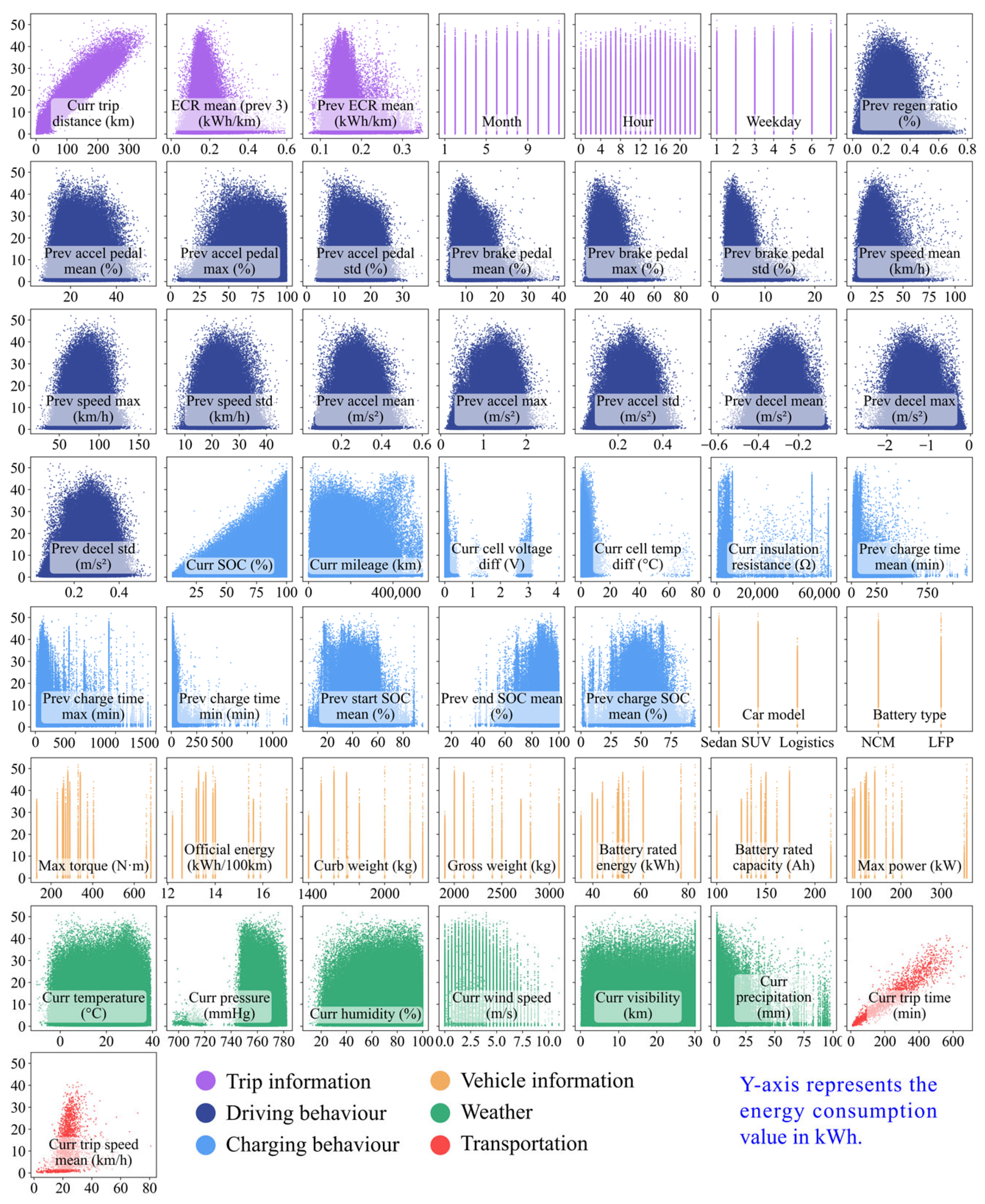
Figure 2. Constructed features and their relationships with energy consumption.
Technologies 13 00493 g002
Figure 3. The inconsistent feature spaces for different downstream tasks.
Technologies 13 00493 g003
Figure 4. Energy consumption prediction accuracy of different models. (a) R2 of test dataset; (b) MAE test dataset.
Technologies 13 00493 g004
Figure 5. Scatter of real and predicted energy consumption of a BEV.
Technologies 13 00493 g005
Figure 6. Ablation analysis of the IFS-Former. (a) R2 of test dataset; (b) MAE test dataset.
Technologies 13 00493 g006
Figure 7. Interpretability analysis of the IFS-Former. (a) Grouped average contributions; (b) Grouped total contributions.
Technologies 13 00493 g007
Table 1. Details and examples of the original datasets.
CategoriesDetails
Real-time
vehicle
records
Collection timeCityStatus (Run, Charge, Park)
13 July 2023 07:03:09ShanghaiRun
Sum mileage (km)Sum votage (V)Max battery single Temp (°C)
92,735338.226
State of charge (%)Sum current (A)Min battery single Temp (°C)
7330.917
Speed (km/h)Accelerator pedal (%)Max battery single voltage (V)
53364.1
Insulation resistance (Ω)Brake padel (%)Min battery single voltage (V)
666803.1
Vehicle informationMax power (kW)Max torque (N∙m)Model (SUV, Sedan, Logistics)
220465Sedan
Curb weight (kg)Battery rated capacity (Ah)Battery type (NCM, LFP)
1850150NCM
Gross weight (kg)Battery rated energy (kWh)Official energy (kWh/100 km)
23507513.5
WeatherTimeTemperature (°C)Pressure (mmHg)Visibility (km)
12 July 2023 23:00:002776015
Precipitation (mm)Humidity (%)Wind speed (m/s)City
0563Shanghai
Table 2. Trip distances and corresponding weights.
CategoryTrip Distance (km)Total Number w e i g h t q
Short trips0 ≤ d < 16173,0830.949
Ordinary trips16 ≤ d < 100237,2520.692
Long tripsd ≥ 10082,4991.991
Table 3. Metrics of energy consumption prediction results in downstream tasks.
MethodFew-ShotR2BiasMAERMSEMAPE
MLR3840.8231 ± 0.24770.2438 ± 2.70702.9754 ± 1.59803.9616 ± 2.01000.6529 ± 0.6577
M-GPR2560.6454 ± 0.2451−1.1394 ± 3.68724.5983 ± 1.27145.9443 ± 1.98021.2655 ± 1.0998
3840.8194 ± 0.2108−1.2605 ± 2.39113.0778 ± 1.44234.1931 ± 2.22440.6014 ± 0.3241
XG
Boost
320.8073 ± 0.1576−1.4693 ± 1.77273.0696 ± 1.51834.5203 ± 2.21540.3677 ± 0.2344
640.8426 ± 0.1882−1.2654 ± 1.69692.7848 ± 1.55594.0377 ± 2.30770.3541 ± 0.2569
1280.9009 ± 0.0617−0.5644 ± 1.12222.2085 ± 0.72123.3040 ± 1.10220.3009 ± 0.1239
2560.9033 ± 0.0646−0.4790 ± 1.08272.1605 ± 0.55013.2389 ± 0.95760.2936 ± 0.1112
3840.9315 ± 0.0250−0.7053 ± 0.77451.8895 ± 0.51672.8442 ± 0.74860.2168 ± 0.0492
Light
GBM
1280.8506 ± 0.1224−0.4134 ± 1.73302.8047 ± 1.17913.9648 ± 1.58780.4680 ± 0.3204
2560.9195 ± 0.0430−0.2591 ± 1.01652.0809 ± 0.60863.0246 ± 0.89210.2917 ± 0.1002
3840.9331 ± 0.0482−0.6522 ± 0.71541.8180 ± 0.57462.7466 ± 1.00330.2274 ± 0.0629
ECR × dAll0.9590 ± 0.01140.0330 ± 0.06121.4181 ± 0.35022.2050 ± 0.49540.1420 ± 0.0246
IFS-
Former
00.9741 ± 0.0087−0.0791 ± 0.38151.1989 ± 0.35131.7674 ± 0.50650.1363 ± 0.0343
320.9741 ± 0.0086−0.0698 ± 0.37991.1987 ± 0.34911.7665 ± 0.50380.1369 ± 0.0346
640.9741 ± 0.0088−0.0629 ± 0.38741.1985 ± 0.34931.7668 ± 0.50600.1366 ± 0.0339
1280.9739 ± 0.0092−0.0509 ± 0.41431.2012 ± 0.35401.7722 ± 0.51630.1363 ± 0.0324
2560.9740 ± 0.0083−0.0543 ± 0.41161.2004 ± 0.34931.7723 ± 0.50440.1379 ± 0.0353
3840.9743 ± 0.0083−0.0669 ± 0.40461.1954 ± 0.34951.7638 ± 0.50440.1361 ± 0.0325
Disclaimer/Publisher’s Note: The statements, opinions and data contained in all publications are solely those of the individual author(s) and contributor(s) and not of MDPI and/or the editor(s). MDPI and/or the editor(s) disclaim responsibility for any injury to people or property resulting from any ideas, methods, instructions or products referred to in the content.