Fibonacci Tessellation for Optimizing Planar Phased Arrays in Satellite Communications

Abstract

This article presents a novel strategy for the design of planar phased arrays using Fibonacci-based partitioning combined with a random multi-objective search. This approach intends to minimize the number of phase shifters used by the system while maintaining the radiation characteristics required for Ku-band user terminals in Low Earth Orbit (LEO) satellite communications. This methodology efficiently tessellates a $16\times 16$ antenna array, reducing the solution search space size and improving algorithmic computational time. From a total of 409,600 possible configurations, an optimal candidate solution was obtained in 2 h. This configuration achieves a balanced trade-off between radiation performance metrics, including side lobe level (SLL), first null beamwidth (FNBW), and the number of phase shifters. This optimal design maintains a value of SLL below $-15$ dB across all the azimuth scanning angles, with a beam steering capability of $\theta =-{40}^{\circ }$ and $0^{\circ }\le \varphi \le {360}^{\circ }$. These results demonstrate the suitability of this novel approach regarding Ku-band satellite communications, providing efficient and practical solutions for high-demand internet services via LEO satellite systems.

1. Introduction

Phased array antennas have become a relevant technology in modern communication systems, with the capacity to enable dynamic beam steering, wide angle coverage, and robust connectivity between last-generation devices [1]. A traditional design approach for planar phased arrays consists of a periodic element distribution, which can produce undesirable sidelobe levels (SLLs) and limited scanning of the mainlobe. In order to address these limitations, some works have explored unconventional element arrangements that are inspired by mathematical sequences and quasiperiodic structures [2].

Random or fractal repetition techniques have proven to be a faster method for synthesis due to the relatively small number of designs to explore. Moreover, these techniques significantly reduce the number of phase shifters [3], in some cases by up to $75\%$, by grouping a high number of elements per subarray [4]. However, these methodologies have shown limited scanning capability in the azimuth plane, which makes them unsuitable for real-time satellite tracking.

The Fibonacci sequence has been employed as an alternative design component due to its intrinsic quasi-ordered nature, enabling a more diverse distribution of antenna elements compared to regular or conventional grids [5,6,7]. The intrinsic flexibility of the Fibonacci methodology allows designers to achieve array compactness while introducing controlled diversity that enhances the beam steering performance and simultaneously mitigates pattern distortions across large scanning angles.

Recent works have demonstrated that applying deterministic aperiodic tiling in planar phased array designs leads to significant improvements in pattern stability under two-dimensional scanning [8,9], particularly in wide-angle scenarios that are relevant for X and Ku bands in satellite communication systems [10,11,12]. Other authors have chosen to embed structural information and hardware restrictions prior to system design [13,14], reducing the dimensionality of the search space. Furthermore, Fibonacci methodologies enable the synthesis of antenna arrays that balance different parameters, such as sidelobe suppression, scan coverage, and radiation efficiency, while reducing the system complexity of the feeding network in terms of phase-shifting components.

This work presents a comprehensive analysis of the design of planar phased antenna arrays through a novel Fibonacci approach, emphasizing radiation performance, wide scanning capabilities, and structural simplicity over other conventional and uniform approaches. Fibonacci configurations enable maintaining global structural coherence, ensuring predictable radiation behavior based on geometric mirror properties while minimizing the number of solutions in the optimization design space. These benefits make Fibonacci designs highly attractive for use in the next generation of satellite user terminals and ground stations that require compact and high-performance phased arrays.

The main scope of this paper is to provide a system-level optimization framework focusing on the design problem, leveraging low algorithmic computational time produced by the implementation of initial constraints in the combinatorial subarray arrangement. Thus, search spaces that would be unattainable by exhaustive approaches are partially explored by using bio-inspired random algorithms as a means of obtaining feasible solutions in a reasonable amount of time.

2. Methodology

In order to enable wide-angle beam steering of the mainlobe in real time, which is demanded by LEO ground terminals [15], while minimizing control and structural complexity, a novel bio-inspired tessellation strategy that constrains the subarray distribution by using the Fibonacci sequence is presented. This provides a structured and diverse search space of solutions that preserves radiation properties due to the geometry of designs, reduction in the number of phase shifters, and compatibility with the scan requirements of satellite systems.

2.1. Problem Statement

Consider a planar phased array as a user terminal that requires wide-angle beam steering across the elevation plane in the interval $[-{40}^{\circ }\le \theta \le 0^{\circ }]$ and full azimuthal scanning in $[0^{\circ }\le \varphi \le {360}^{\circ }]$ for satellite tracking. Let the array have $N\times M$ antenna elements on a quadrangular grid with spacings of $d_x=d_y=\lambda /2$. The main objective is to generate robust scanning patterns with low SLL and reduced FNBW while retaining a practical control architecture. In this paper, the number of control ports is treated as a constraint rather than an optimization objective.

The array factor of the planar array is defined as a function of the scan angle direction (${\theta }_0$, ${\varphi }_0$) given by

$$AF({\theta }_0,{\varphi }_0)=\sum _{n=1}^N\sum _{m=1}^M{I}_{n,m}{e}^{j[kd(n-1){\psi }_x+kd(m-1){\psi }_y+{\beta }_x+{\beta }_y]},$$

(1)

where

$${\psi }_x=sin\theta +cos\varphi ,{\psi }_y=sin\theta +sin\varphi$$

(2)

$${\beta }_x=-kd(n-1)sin{\theta }_{0}cos{\varphi }_0$$

(3)

$${\beta }_y=-kd(m-1)sin{\theta }_{0}sin{\varphi }_0.$$

(4)

with $k=2\pi /\lambda$, and the antenna element factor is treated as an isotropic element for synthesis.

The complex excitation $I_{n,m}$ employs raised-cosine window tapering using the array center as a reference to calculate the distance $d_{n,m}$ of each element, defined by

$$I_{n,m}={\displaystyle \frac{1}{2}}\left[1+cos\left({\displaystyle \frac{d_{n,m}{cos}^{-1}(2a-1)}{0.5L}}\right)\right]$$

(5)

where

$$d_{n,m}=\sqrt{d{x}_{n,m}^2+d{y}_{n,m}^2}$$

(6)

with L as the aperture length and $a=0.14$ chosen by symmetry. The tapering function is normalized for convention, which enables decay of amplitudes from the array center to the edges. This stabilizes the SLL without compromising the mainlobe performance while scanning across the plane.

In the context of subarray distribution, the same distance equation applies by using an average distance of each subarray (centroid) to the array center, replacing $d_{n,m}$ with

$$d_c=\sqrt{{\left({\displaystyle \frac{1}{N_s}}\sum _{i=1}^{N_s}d{x}_i\right)}^2+{\left({\displaystyle \frac{1}{N_s}}\sum _{i=1}^{N_s}d{y}_i\right)}^2}$$

(7)

while preserving a smoother taper despite an irregular subarray distribution and geometric shape. The centroid distance is computed by averaging each element coordinate of each subarray with $N_s$ elements and then using that distance in the raised-cosine tapering equation expressed in (5).

A convenient representation of an $N\times M$ planar phased array is by using a matrix of $P{S}_m\times M$ integers, where each number corresponds to the number of antenna elements grouped into a subarray $K_j$ of size j. This abstraction enables simplifying the design process by reducing the planar array configuration into a discrete mathematical structure that embeds the size and distribution of the subarrays across rows and columns in the matrix [11]. In this representation, each row $m\in \{1,2,\dots ,M-1,M\}$ of the matrix can be viewed as a linear array partitioned into subarrays, such that $P{S}_m=\sum K_j$, and the total number of phase shifters required by the system is obtained by the sum of the number of integers across the entire matrix.

$$P{S}_{\mathrm{total}}=\sum _{m=1}^{M}P{S}_m$$

(8)

2.2. Random Approach

An efficient exploration of the solution space is achieved by integrating random search algorithms and evolutionary strategies to approximate a Pareto-optimal set. For an unconstrained case, the size of the search space $\mathcal{S}$ is given by

$$\mathcal{S}={\displaystyle \frac{(s+M-1)!}{M!(s-1)!}},$$

(9)

where M represents the number of rows in the planar array and s the number of possible linear array sequences of integer numbers. This mathematical framework shows the exponential growth of the search space with the large increment of the array size M, and the number of possible combinations due to the variation in subarray sizes $K_j$, where $j\in J\subset \mathbb{N}$, justifying from the latter the need for metaheuristics and multi-objective approaches in order to avoid exhaustive computation [16].

$$s={\displaystyle \frac{\left(P{S}_m\right)!}{{\displaystyle \prod _{j\in J\subset \mathbb{N}}}\left(K_j\right)!}}$$

(10)

Assuming that each row sequence $S_m$ admits the same type of integer compositions $C_m$ to partition the N elements of a row into permissible subarray sizes $K_j$, the number of different planar designs is provided by a row-wise matrix multiplication of multinomial operations, producing the same factor s in (10) repeated M times, considering that the number of subarrays per row $P{S}_m=\sum K_j$ is identical for all rows; therefore,

$$\mathcal{S}=\prod _{m=1}^M\left({\displaystyle \frac{\left(P{S}_m\right)!}{{\displaystyle \prod _{j\in J\subset \mathbb{N}}}\left(K_j\right)!}}\right)={\left({\displaystyle \frac{\left(P{S}_m\right)!}{{\displaystyle \prod _{j\in J\subset \mathbb{N}}}\left(K_j\right)!}}\right)}^M.$$

(11)

However, in some cases, the number of rows may differ based on the type of permissible compositions. In that case, it is necessary to count the number of possible sequences $s_k$ for each row in m that are generated by the compositions contained in the subset $C_m$ and then calculate the product of all the rows by

$$\mathcal{S}=\prod _{m=1}^M\left(\sum _{k=1}^{|C_m|}{s}_k\right).$$

(12)

This calculation shows how variations in the subarray combinations impact the full array diversity and makes clear the role of the number of phase shifters embedded in $P{S}_m$.

2.3. Fibonacci Partitioning and Tessellation

A new discrete framework for the design of planar phased arrays based on the Fibonacci sequence is introduced in this work, which is intended to generate fast and feasible planar array designs from a discrete and constrained mathematical perspective. This approach offers the designer some advantages over random unconstrained methods, such as the ability to determine beforehand the number of phase lines for the feeding network or to choose the permissible sizes of subarrays in the array.

The Fibonacci sequence is a series of integer numbers where each number is the sum of the two preceding ones [17], defined by

$$F_n=F_{n-1}+F_{n-2},$$

(13)

where $F_0=0$ and $F_1=1$. The scalability of this methodology is bounded by multiples of this sequence embedded in the dimensions of the $N\times M$ quadrangular array. Thus, the total number of antenna elements per axis in the matrix is given by

$$N=M=(F_n+F_{n-3})\mid n\ge 3.$$

(14)

The latter expression restricts the dimensions of the achievable planar array designs to the sequence $N=M\in \{2,4,6,10,16,26,42\dots \}$, providing a discrete boundary for both antenna elements and phase shifters prior to the search for optimal solutions.

For purposes of this work, the planar array consists of $16\times 16$ antenna elements; therefore, the Fibonacci sequence is defined by $F_n=\{0,1,1,2,3,5,8,13\}$ for $2\le n\le 7$. The array is partitioned into four symmetric segments to facilitate the replication of the optimal solutions of subproblems and to ensure geometric mirroring properties during scanning. On each segment, seven combinatorial subproblems are defined, ensuring that the number of antenna elements per row is delimited by $N_s\in \{3,5,8,13\}$ from $F_2$ to $F_7$.

Linear subproblems are structured by rows, where the top linear bands use $N_s=13$ antenna elements per row (set $C_b=C_1\cup C_2\cup C_3$), the middle subproblems with $N_s=8$ (set $C_a=C_4\cup C_5$), the lower linear band with $N_s=5$ (set $C_6$), and the two innermost linear subproblems are composed of equally excited elements $N_s\in \{1,3\}$ (sets $C_7$ and $C_8$). This produces a geometric tessellation across the array that simplifies the synthesis structure by repeating four symmetric segments.

For example, consider that a $16\times 16$ planar array can be partitioned into smaller subproblems for simplification, as illustrated in Figure 1. In this case, six linear array subproblems or sequences are generated, taking into account the fixed antenna elements for $C_8=\left\{1\right\}$ and $C_7=\{1,1,1\}$. The maximum number of antenna elements per subarray is constrained by $1\le j\le 5$, which enables generating the following partitions. For the case of set $C_b$, the subset compositions are defined as $C_b\in \{\{5,5,3\},\{5,4,4\},\{5,4,3,1\}\}|N_s=13$. For the set $C_a$, the subset is given by $C_a=\{2,2,2,1,1\}|N_s=8$. Finally, for subset $C_6$, the subset is $C_6=\{2,2,1\}|N_s=5$. According to (11) and (12), the total number of possible solutions resulting from this configuration of compositions is given by

$$\mathcal{S}=\prod _{n=5}^7{\left(\sum _{|C_m|<C_k\left(N_s\right)}{\displaystyle \frac{\left(P{S}_m\right)!}{{\displaystyle \prod _{j\in J\subset \mathbb{N}}}\left(K_j\right)!}}\right)}^{F_{n-3}}$$

(15)

where $C_k\left(N_s\right)$ denotes the number of all possible partitions of $N_s$ without restrictions in J array sizes. Therefore,

$$\mathcal{S}={\left(\left({\displaystyle \frac{3!}{2!}}\right)+\left({\displaystyle \frac{3!}{2!}}\right)+\left({\displaystyle \frac{4!}{1!}}\right)\right)}^3·{\left({\displaystyle \frac{5!}{3!·2!}}\right)}^2·\left({\displaystyle \frac{3!}{2!}}\right)=8,100,000.$$

(16)

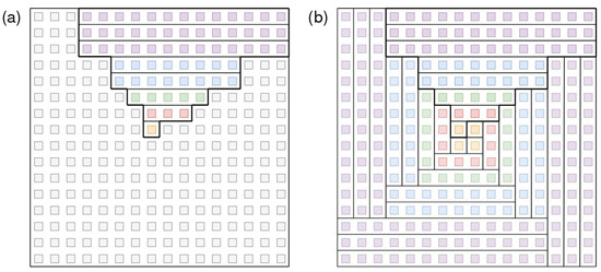
Figure 1. Fibonacci tessellation and combinatorial subproblems for a $16\times 16$ planar array. In (a), one of the four symmetric segments is shown as a “staircase” pattern. The colored sections in the array represent the eight linear subproblems created by the Fibonacci-inspired methodology; from the center to ends, 1 in yellow, 3 in red, 5 in green, 8 in two rows of blue, and 13 in three rows of violet. In (b), the full tessellation is obtained by mirroring and rotating the first segment into the remaining three, producing a fourfold symmetric template over the quadrangular $16\times 16$ grid.

In order to provide insight about the exponential growth of an unconstrained solution search space, consider that each subproblem in the segment can be partitioned as the maximum size of the subproblem itself; therefore, the total number of solutions for the unconstrained case is given by $\left({4096}^3\right)\left({128}^2\right)\left(16\right)\left(4\right)\approx 7.21\times {10}^{16}$. Taking into account that each solution is computed with an average time of 20 ms, this search would take approximately $45.7$ million years to execute using an exhaustive approach. From here, we focus on the importance of discretizing the design problem to exhaustively search bounded solution spaces based on user needs and application requirements.

2.4. Multi-Objective Optimization

The design of planar phased arrays can be expressed as a multi-objective optimization problem [18,19] where multiple performance metrics are optimized simultaneously. In this article, the construction of two minimization functions considers three objectives: SLL, FNBW, and the total number of phase shifters $P{S}_{\mathrm{total}}$ ($x_1$, $x_2$, and $x_3$, respectively). Other frameworks or functions can be used to attain the same objectives; however, the proposed functions can adequately represent the desired objectives. Thus, the minimization function $\mathrm{z}$ is defined by

$$\mathrm{minimize}\mathrm{z}=(f_1(x_1,x_2),f_2(x_2,x_3))$$

(17)

where $f_1$ and $f_2$ correspond to the minimization functions, each one composed of two design parameters in conflict such that

$$f_1(x_1,x_2)=(w_1·x_1)+(w_2·x_2)$$

(18)

$$f_2(x_2,x_3)=(w_2·x_2)+\left({\displaystyle \frac{x_3}{N\times M}}\right)$$

(19)

$$w_1={\displaystyle \frac{max\left(\mathrm{SLL}\right)}{min\left(\mathrm{SLL}\right)}}$$

(20)

$$w_2={\displaystyle \frac{min\left(\mathrm{FNBW}\right)}{max\left(\mathrm{FNBW}\right)}}$$

(21)

The main reason for choosing the weights $w_1$ and $w_2$ as parameters of SLL and FNBW levels is to obtain a real number between the interval $0<w_1\le w_2<1$, which is defined according to the ratio between the best and worst stored values in a solution archive, extracted from the search with permissible SLL threshold. These weights are used for the sole purpose of scaling and are not updated during the optimization process.

The evaluation of the Pareto dominance was carried out under the standard condition that a solution ${\mathbf{x}}_i$ dominates ${\mathbf{x}}_j$ if and only if

$$f_m\left({\mathbf{x}}_i\right)\le f_m\left({\mathbf{x}}_j\right)\forall m\in \{1,2\}\mathrm{and}\exists m:f_m\left({\mathbf{x}}_i\right)<f_m\left({\mathbf{x}}_j\right).$$

(22)

This framework ensures a non-dominated solution form the Pareto front [20], where each solution represents a trade-off between the minimization of SLL, FNBW, and the number of phase elements. The selection of optimal candidate solutions is based on their position along the front, providing the designer the flexibility of choosing the most appropriate compromise given a specific application.

3. Simulation Results

This section presents the results obtained for each case previously described. An algorithm programmed in R was used to compute various instances of the problem of designing a $16\times 16$ phased planar antenna array. All the cases were run via a Linux Debian 12 computer system (Waltham, MA, USA) with eight Intel Core i7-8565U @ 1.80 GHz processors and 16 GB of RAM (Santa Clara, CA, USA).

The elevation plane with a range of $[-\pi /2\le \theta \le \pi /2]$ is represented by the x-axis on each graph by using a resolution of $\pi /3600$ points. The y-axis corresponds to the normalized array factor calculated by

$$y=20log10\left({\displaystyle \frac{\left|AF\right|}{max\left(\right|AF\left|\right)}}\right).$$

(23)

For all instances, the innermost subarrays are composed of individually excited elements such as $C_8=\left\{1\right\}$ and $C_7=\{1,1,1\}$. This initial condition reduces the search space by concentrating the exploration on the six remaining subproblems induced by the Fibonacci compositions. Additionally, in all cases, the mainlobe is scanned across the azimuth plane with increments of $\Delta \varphi ={15}^{\circ }$ in the interval $[0^{\circ }\le \varphi \le {360}^{\circ }]$ and $\theta \in [-{40}^{\circ },0^{\circ }]$ in the elevation plane.

The FNBW represents the angular distance between the first two nulls adjacent to the mainlobe in the radiation pattern. It is calculated by searching for the first increment of value in the y-axis, starting at 0 dB (${\theta }_0$), while displacing through the x-axis (representing the elevation plane) in both left and right directions. Each cut of $AF({\theta }_0,\varphi )$ with steps of $\Delta \varphi ={15}^{\circ }$ computes a distinct FNBW value, and, in some cases, an average value considering multiple cuts is calculated.

The phase shifter reduction percentage is defined by the division of the total number of subarrays in the array with respect to the conventional case, where each antenna element is independently fed with amplitude and phase values. Given that the array is divided by four symmetric segments, the phase shifter reduction percentage is calculated by

$$PS\%=100·\left(1-{\displaystyle \frac{\left(4\right)·\left(P{S}_{\mathrm{total}}\right)}{N\times M}}\right),$$

(24)

where $P{S}_{\mathrm{total}}$ represents the total number of subarrays used for all sets $C_m$ of one segment with eight subproblems, such that $1\le m\le 8$.

3.1. Case I: Fibonacci Random Search

For this case, the admissible subarray sizes $K_j$ within each composition $C_m$ for $1\le m\le 6$ are limited to $j\in \{1,2,3,4\}$. This unrestricted set increases the diversity of designs but also expands the size of the combinatorial search space. A valid configuration was reached after $17.41$ min of computational time, yielding a radiation pattern with symmetric characteristics across different scanning angles, as shown in Figure 2.

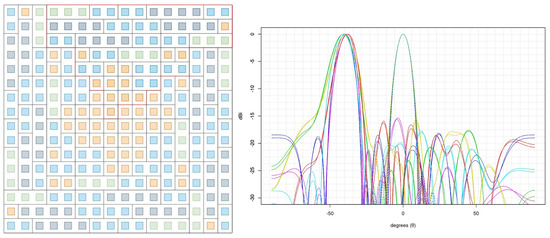
Figure 2. Radiation pattern and design of the $16\times 16$ planar phased array obtained in Case I. The broadside response is shown with dashed lines. The elevation scan range is $\theta \in [-{40}^{\circ },0^{\circ }]$, and the azimuth scan interval is [$0^{\circ }\le \varphi \le {360}^{\circ }$]. The color palette of the radiation patterns represents angular steps of $\Delta \varphi ={15}^{\circ }$, as listed in Table 1.

The design achieves elevation scanning up to $-{40}^{\circ }$ and full azimuth scanning in the interval $[0^{\circ }\le \varphi \le {360}^{\circ }]$. On average, the sidelobe level remained at ${\mathrm{SLL}}_{\mathrm{avg}}=-16.87$ dB with a first null beamwidth of ${\mathrm{FNBW}}_{\mathrm{avg}}=0.91$ radians. The SLL remained below $-15$ dB across all azimuth plane directions, showing the ability of the Fibonacci tessellation technique to preserve radiation performance while substantially reducing the number of phase shifters by $48.44\%$ compared to the conventional case.

Table 1. Results of SLL and FNBW for the planar phased array shown in Figure 2.

$\mathit{\varphi }$	SLL (dB)	FNBW (rad)	Color
$0^{\circ }$, ${180}^{\circ }$	$-18.35$	$0.4433$	Blue
${15}^{\circ }$, ${195}^{\circ }$	$-15.35$	$0.4695$	Magenta
${30}^{\circ }$, ${210}^{\circ }$	$-15.93$	$0.9975$	Red
${45}^{\circ }$, ${225}^{\circ }$	$-15.61$	$1.3142$	Yellow
${60}^{\circ }$, ${240}^{\circ }$	$-17.60$	$1.6511$	Green
${75}^{\circ }$, ${255}^{\circ }$	$-17.70$	$0.5960$	Cyan
${90}^{\circ }$, ${270}^{\circ }$	$-18.13$	$0.4512$	Blue
${105}^{\circ }$, ${285}^{\circ }$	$-15.62$	$0.4773$	Magenta
${120}^{\circ }$, ${300}^{\circ }$	$-16.26$	$0.9913$	Red
${135}^{\circ }$, ${315}^{\circ }$	$-16.07$	$1.3177$	Yellow
${150}^{\circ }$, ${330}^{\circ }$	$-17.77$	$1.6214$	Green
${165}^{\circ }$, ${345}^{\circ }$	$-17.99$	$0.5890$	Cyan

Table 1. Results of SLL and FNBW for the planar phased array shown in Figure 2.

$\mathit{\varphi }$	SLL (dB)	FNBW (rad)	Color
$0^{\circ }$, ${180}^{\circ }$	$-18.35$	$0.4433$	Blue
${15}^{\circ }$, ${195}^{\circ }$	$-15.35$	$0.4695$	Magenta
${30}^{\circ }$, ${210}^{\circ }$	$-15.93$	$0.9975$	Red
${45}^{\circ }$, ${225}^{\circ }$	$-15.61$	$1.3142$	Yellow
${60}^{\circ }$, ${240}^{\circ }$	$-17.60$	$1.6511$	Green
${75}^{\circ }$, ${255}^{\circ }$	$-17.70$	$0.5960$	Cyan
${90}^{\circ }$, ${270}^{\circ }$	$-18.13$	$0.4512$	Blue
${105}^{\circ }$, ${285}^{\circ }$	$-15.62$	$0.4773$	Magenta
${120}^{\circ }$, ${300}^{\circ }$	$-16.26$	$0.9913$	Red
${135}^{\circ }$, ${315}^{\circ }$	$-16.07$	$1.3177$	Yellow
${150}^{\circ }$, ${330}^{\circ }$	$-17.77$	$1.6214$	Green
${165}^{\circ }$, ${345}^{\circ }$	$-17.99$	$0.5890$	Cyan

The experimental results of this case demonstrate that the proposed methodology based on random sequences of linear arrays contained in subproblems allows the array to have enriched design diversity. Although this technique reduces the number of phase shifters in the system, it still uses more than half compared to the conventional case. Consequently, an alternative Fibonacci tessellation is proposed with a more restricted set of compositions. This broader search aims to achieve a more reduced number of phase shifters without sacrificing SLL and FNBW of the mainlobe.

3.2. Case II: Search Space with 81 Solutions

In order to obtain an optimal design within a practical execution runtime, the search begins from a relatively small candidate set. For the linear array subproblems with $N_s=13$, the subarray composition $C_b=\{5,5,3\}$ is selected with sequence $C_a=\{2,2,2,2\}$ fixed and set $C_6=\{2,2,1\}$. An exhaustive search of solutions is later conducted given the reduced size of the search space. Likewise, a multi-objective optimization approach was adopted for the evaluation of candidate solutions by using (17), thus enabling the identification of multiple configurations with suitable electromagnetic performance to address the design problem.

In the search space 81-1, a global optimal solution was found with a computational time of 2.04 s. This solution is not dominated by any other in the search space according to the dominance expression defined in (22). The resulting design enables scanning of $\theta =-{40}^{\circ }$ in the elevation plane and full azimuth scanning in the interval $[0^{\circ }\le \varphi \le {360}^{\circ }]$ while maintaining an SLL below a $-12$ dB threshold, as shown in Table 2. The resulting planar array configuration and its radiation pattern are illustrated in Figure 3.

Table 2. Results of SLL and FNBW for the planar phased array shown in Figure 3.

$\mathit{\varphi }$	SLL (dB)	FNBW (rad)	Color
$0^{\circ }$, ${90}^{\circ }$, ${180}^{\circ }$, ${270}^{\circ }$	$-13.23$	$0.3978$	Blue
${15}^{\circ }$, ${105}^{\circ }$, ${195}^{\circ }$, ${285}^{\circ }$	$-15.09$	$0.4508$	Magenta
${30}^{\circ }$, ${120}^{\circ }$, ${210}^{\circ }$, ${300}^{\circ }$	$-13.98$	$0.6375$	Red
${45}^{\circ }$, ${135}^{\circ }$, ${225}^{\circ }$, ${315}^{\circ }$	$-14.65$	$1.1884$	Yellow
${60}^{\circ }$, ${150}^{\circ }$, ${240}^{\circ }$, ${330}^{\circ }$	$-18.49$	$1.2939$	Green
${75}^{\circ }$, ${165}^{\circ }$, ${255}^{\circ }$, ${345}^{\circ }$	$-12.17$	$0.6602$	Cyan

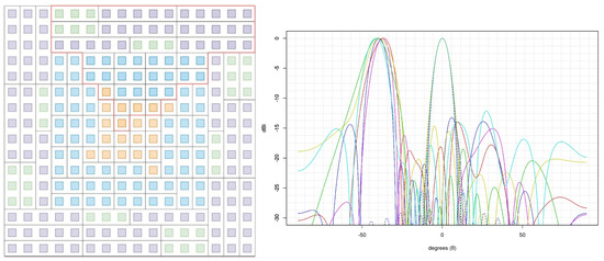
Figure 3. Radiation pattern and design of the $16\times 16$ planar phased array obtained in Case II-1. The broadside response is shown with dashed lines. The elevation scan range is $\theta \in [-{40}^{\circ },0^{\circ }]$, and the azimuth scan interval is $[0^{\circ }\le \varphi \le {360}^{\circ }]$. The color palette of the radiation patterns represents angular steps of $\Delta \varphi ={15}^{\circ }$, as listed in Table 2.

In order to compare different designs under a fixed number of phase shifters, a second set of compositions was selected to replace $C_b$ with $\{5,4,4\}$, which preserves the same size of the solution space and the same total number of phase shifters while offering a different type of design. The exhaustive search was performed with a computational time of 1.91 s. In contrast to the search space 81-1, a Pareto front with four solutions was successfully obtained for this instance, with similar scanning capabilities in the elevation plane for $\theta =-{40}^{\circ }$ and azimuth plane interval $[0^{\circ }\le \varphi \le {360}^{\circ }]$, while maintaining an SLL below $-12$ dB.

One candidate solution was selected from a Pareto front (four solutions), obtained from an exhaustive search of the space 81-2 for a comparison to the global optimal solution of space 81-1. The comparison was performed by calculating the average SLL and FNBW for all angular steps of $\Delta \varphi ={15}^{\circ }$ in the azimuth plane for both solutions. In space 81-1, averages of ${\mathrm{SLL}}_{\mathrm{a}1}=-14.60$ dB and ${\mathrm{FNBW}}_{\mathrm{a}1}=0.7714$ rad were obtained, while the solution from space 81-2 (shown in Figure 4) reported averages of ${\mathrm{SLL}}_{\mathrm{a}2}=-13.14$ dB and ${\mathrm{FNBW}}_{\mathrm{a}2}=0.6966$ rad. Both solutions consist of a total of 96 subarrays, representing a $62.5\%$ reduction in the number of phase shifters compared to the conventional case.

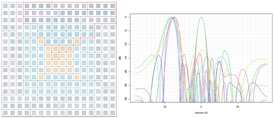
Figure 4. Radiation pattern and design of the $16\times 16$ planar phased array obtained in Case II-2. The broadside response is shown with dashed lines. The elevation scan range is $\theta \in [-{40}^{\circ },0^{\circ }]$, and the azimuth scan interval is $[0^{\circ }\le \varphi \le {360}^{\circ }]$. The color palette of the radiation patterns represents angular steps of $\Delta \varphi ={15}^{\circ }$, as listed in Table 3.

Table 3. Results of SLL and FNBW for the planar phased array shown in Figure 4.

$\mathit{\varphi }$	SLL (dB)	FNBW (rad)	Color
$0^{\circ }$, ${90}^{\circ }$, ${180}^{\circ }$, ${270}^{\circ }$	$-14.04$	$0.3944$	Blue
${15}^{\circ }$, ${105}^{\circ }$, ${195}^{\circ }$, ${285}^{\circ }$	$-13.62$	$0.4660$	Magenta
${30}^{\circ }$, ${120}^{\circ }$, ${210}^{\circ }$, ${300}^{\circ }$	$-13.24$	$0.6857$	Red
${45}^{\circ }$, ${135}^{\circ }$, ${225}^{\circ }$, ${315}^{\circ }$	$-11.87$	$1.1886$	Yellow
${60}^{\circ }$, ${150}^{\circ }$, ${240}^{\circ }$, ${330}^{\circ }$	$-12.21$	$0.8966$	Green
${75}^{\circ }$, ${165}^{\circ }$, ${255}^{\circ }$, ${345}^{\circ }$	$-13.83$	$0.5483$	Cyan

Table 3. Results of SLL and FNBW for the planar phased array shown in Figure 4.

$\mathit{\varphi }$	SLL (dB)	FNBW (rad)	Color
$0^{\circ }$, ${90}^{\circ }$, ${180}^{\circ }$, ${270}^{\circ }$	$-14.04$	$0.3944$	Blue
${15}^{\circ }$, ${105}^{\circ }$, ${195}^{\circ }$, ${285}^{\circ }$	$-13.62$	$0.4660$	Magenta
${30}^{\circ }$, ${120}^{\circ }$, ${210}^{\circ }$, ${300}^{\circ }$	$-13.24$	$0.6857$	Red
${45}^{\circ }$, ${135}^{\circ }$, ${225}^{\circ }$, ${315}^{\circ }$	$-11.87$	$1.1886$	Yellow
${60}^{\circ }$, ${150}^{\circ }$, ${240}^{\circ }$, ${330}^{\circ }$	$-12.21$	$0.8966$	Green
${75}^{\circ }$, ${165}^{\circ }$, ${255}^{\circ }$, ${345}^{\circ }$	$-13.83$	$0.5483$	Cyan

3.3. Case III: Search Space with 10,648 Solutions

For this instance, only the compositions in set $C_b$ are varied. The remainder of the subproblem segments are fixed for sets $C_b\in \{\{5,5,3\},\{5,4,4\},\{4,4,4,1\},\{4,4,3,2\}\}$, while the other compositions are also fixed for sets $C_a=\{2,2,2,2\}$ and $S_6=\{2,1,2\}$. The exhaustive search resulted in a global optimal solution obtained with a computational time of 3.82 min and average performance values of ${\mathrm{SLL}}_{\mathrm{avg}}=-15.85$ dB and ${\mathrm{FNBW}}_{\mathrm{avg}}=0.8364$ rad.

The results presented in Table 4 describe a configuration with elevation scanning capability of $\theta =-{40}^{\circ }$ and mainlobe steering in the azimuth plane within the interval $[0^{\circ }\le \varphi \le {360}^{\circ }]$ while maintaining an SLL below a $-14$ dB threshold. The resulting planar array design shown in Figure 5, is composed of 108 subarrays, achieving a $57.81\%$ reduction in the number of phase shifters compared to the conventional case.

Table 4. Results of SLL and FNBW for the planar phased array shown in Figure 5.

$\mathit{\varphi }$	SLL (dB)	FNBW (rad)	Color
$0^{\circ }$, ${90}^{\circ }$, ${180}^{\circ }$, ${270}^{\circ }$	$-14.36$	$0.4110$	Blue
${15}^{\circ }$, ${105}^{\circ }$, ${195}^{\circ }$, ${285}^{\circ }$	$-17.32$	$0.4383$	Magenta
${30}^{\circ }$, ${120}^{\circ }$, ${210}^{\circ }$, ${300}^{\circ }$	$-19.48$	$0.7141$	Red
${45}^{\circ }$, ${135}^{\circ }$, ${225}^{\circ }$, ${315}^{\circ }$	$-14.63$	$1.6822$	Yellow
${60}^{\circ }$, ${150}^{\circ }$, ${240}^{\circ }$, ${330}^{\circ }$	$-15.21$	$1.2029$	Green
${75}^{\circ }$, ${165}^{\circ }$, ${255}^{\circ }$, ${345}^{\circ }$	$-14.07$	$0.5701$	Cyan

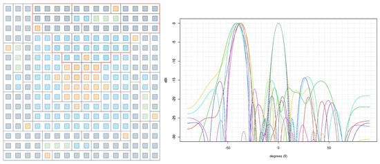
Figure 5. Radiation pattern and design of the $16\times 16$ planar phased array obtained in Case III. The broadside response is shown with dashed lines. The elevation scan range is $\theta \in [-{40}^{\circ },0^{\circ }]$, and the azimuth scan interval is [$0^{\circ }\le \varphi \le {360}^{\circ }$]. The color palette of the radiation patterns represents angular steps of $\Delta \varphi ={15}^{\circ }$, as listed in Table 4.

3.4. Case IV: Search Space with 409,600 Solutions

For the final instance of the problem, both sets $C_b$ and $C_a$ were modified as $N_s=13$, $C_b\in \{\{5,3,3,2\},\{4,4,4,1\}\}$, and $N_s=8$, $C_b=\{2,2,2,1,1\}$. A Pareto front with 11 candidate solutions was obtained from an exhaustive search of a space containing 409,600 solutions, computed with an execution time of 2.01 h. For comparative purposes, two solutions, $s^{\left(1\right)}$ and $s^{\left(2\right)}$, were selected from this front for detailed analysis, following a procedure similar to the one described in Case II. The permissible SLL threshold for both solutions was set to $-15$ dB, with a fixed number of 116 subarrays, representing a $54.69\%$ reduction in the total number of phase shifters required by the system.

The first solution $s^{\left(1\right)}$ was selected from the central region of the Pareto front and reported average values of ${\mathrm{SLL}}_{\mathrm{a}1}=-16.92$ dB and ${\mathrm{FNBW}}_{\mathrm{a}1}=0.5666$ rad. The results are summarized in Table 5 and show that solution $s^{\left(1\right)}$ provides an elevation scanning capability of $\theta =-{40}^{\circ }$, with a mainlobe steering in the azimuth plane of $[0^{\circ }\le \varphi \le {360}^{\circ }]$, while maintaining SLL values below a $-15$ dB threshold. The resulting planar array configuration and its radiation pattern are illustrated in Figure 6.

Table 5. Results of SLL and FNBW for the planar phased array shown in Figure 6.

$\mathit{\varphi }$	SLL (dB)	FNBW (rad)	Color
$0^{\circ }$, ${90}^{\circ }$, ${180}^{\circ }$, ${270}^{\circ }$	$-16.75$	$0.4241$	Blue
${15}^{\circ }$, ${105}^{\circ }$, ${195}^{\circ }$, ${285}^{\circ }$	$-16.09$	$0.4616$	Magenta
${30}^{\circ }$, ${120}^{\circ }$, ${210}^{\circ }$, ${300}^{\circ }$	$-18.20$	$0.7461$	Red
${45}^{\circ }$, ${135}^{\circ }$, ${225}^{\circ }$, ${315}^{\circ }$	$-15.83$	$1.2139$	Yellow
${60}^{\circ }$, ${150}^{\circ }$, ${240}^{\circ }$, ${330}^{\circ }$	$-16.28$	$1.0472$	Green
${75}^{\circ }$, ${165}^{\circ }$, ${255}^{\circ }$, ${345}^{\circ }$	$-18.39$	$0.5541$	Cyan

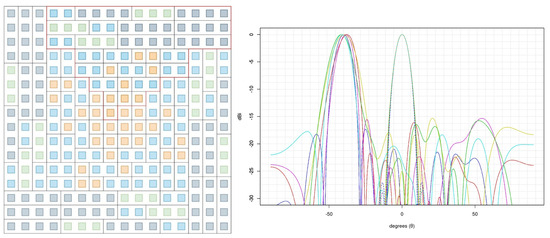
Figure 6. Radiation pattern and design of the $16\times 16$ planar phased array obtained in Case IV-1. The broadside response is shown with dashed lines. The elevation scan range is $\theta \in [-{40}^{\circ },0^{\circ }]$, and the azimuth scan interval is [$0^{\circ }\le \varphi \le {360}^{\circ }$]. The color palette of the radiation patterns represents angular steps of $\Delta \varphi ={15}^{\circ }$, as listed in Table 5.

The second solution $s^{\left(2\right)}$ achieved the best performance on objective $f_1$, with average values of ${\mathrm{SLL}}_{\mathrm{a}2}=-16.26$ dB and ${\mathrm{FNBW}}_{\mathrm{a}2}=0.6741$ rad. The results shown in Table 6 demonstrate that solution $s^{\left(2\right)}$ also provides elevation scanning of $\theta =-{40}^{\circ }$, with full azimuth scanning in the interval $[0^{\circ }\le \varphi \le {360}^{\circ }]$, while maintaining SLL values below $-15$ dB, as illustrated in Figure 7.

Table 6. Results of SLL and FNBW for the planar phased array shown in Figure 7.

$\mathit{\varphi }$	SLL (dB)	FNBW (rad)	Color
$0^{\circ }$, ${90}^{\circ }$, ${180}^{\circ }$, ${270}^{\circ }$	$-17.33$	$0.4241$	Blue
${15}^{\circ }$, ${105}^{\circ }$, ${195}^{\circ }$, ${285}^{\circ }$	$-15.33$	$0.4913$	Magenta
${30}^{\circ }$, ${120}^{\circ }$, ${210}^{\circ }$, ${300}^{\circ }$	$-16.10$	$0.7034$	Red
${45}^{\circ }$, ${135}^{\circ }$, ${225}^{\circ }$, ${315}^{\circ }$	$-15.30$	$0.9660$	Yellow
${60}^{\circ }$, ${150}^{\circ }$, ${240}^{\circ }$, ${330}^{\circ }$	$-15.75$	$0.9407$	Green
${75}^{\circ }$, ${165}^{\circ }$, ${255}^{\circ }$, ${345}^{\circ }$	$-17.74$	$0.5192$	Cyan

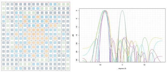
Figure 7. Radiation pattern and design of the $16\times 16$ planar phased array obtained in Case IV-2. The broadside response is shown with dashed lines. The elevation scan range is $\theta \in [-{40}^{\circ },0^{\circ }]$, and the azimuth scan interval is [$0^{\circ }\le \varphi \le {360}^{\circ }$]. The color palette of the radiation patterns represents angular steps of $\Delta \varphi ={15}^{\circ }$, as listed in Table 6.

3.5. Geometric Balance by Means of Spatial Moments

For the purpose of verifying that the four-segment replication preserves a geometric scan balance, the discrete spatial moments and product of inertia of the complex excitation distribution $I_{n,m}$ were computed [21], making use of Case I as the design reference. Let $d{x}_{n,m}$ and $d{y}_{n,m}$ be each antenna element coordinate with respect to the array center. Then, the first spatial moments are given by

$$A_x=\sum _{n=1}^N\sum _{m=1}^M{I}_{n,m}d{x}_{n,m},A_y=\sum _{n=1}^N\sum _{m=1}^M{I}_{n,m}d{y}_{n,m}.$$

(25)

while the second moments and product of inertia are denoted as

$$B_x=\sum I_{n,m}d{y}_{n,m}^2,B_y=\sum I_{n,m}d{x}_{n,m}^2,B_{xy}=\sum I_{n,m}d{x}_{n,m}d{y}_{n,m}.$$

(26)

resulting in values of ${\overline{A}}_x={\overline{A}}_y=0.03$ for the normalized first moments, $B_x=B_y=341.7$ for the second moments, and $B_{xy}=341.7$ for the cross moment or product of inertia.

The first results indicate that the array is nearly balanced at broadside but not perfectly centered; this is inferred from a small non-zero value of $0.03$ obtained for the normalized centroids ${\overline{A}}_x={\overline{A}}_y$, which suggests a slight offset. Additionally, the second moments (equal values) indicate that the aperture has an isotropic spread in both the x and y axes, which confirms the array geometric balance. Finally, the product of inertia $B_{xy}$ is different from zero and equal to $B_x$ and $B_y$, which reveals that the symmetry of the tessellation is aligned with the diagonals (${45}^{\circ }$), thus achieving geometric balance at broadside through a diagonal symmetry rather than a conventional symmetry dependent on aligned axes.

4. Discussion and Conclusions

Although several effects, such as mutual coupling and phase quantization, are not addressed within the scope of this work, the Fibonacci tessellation methodology provides indirect structural properties that contribute to mitigating these undesired conditions. The irregular distribution of subarrays enables reducing strong coupling between the nearest elements compared to periodic arrangements added to the raised-cosine tapering, which ensures a flat level of excitation to mitigate element perturbations. Additionally, by reducing the number of phase shifters, this approach minimizes the total impact of quantization, which can be validated in future work under realistic implementation constraints.

Practical phased array implementations in satellite applications require diligent RF calibration due to parameters such as gain and phase errors introduced by the RF chains. Some works addressed this problem by proposing algorithms to calibrate wideband multi-antenna satellites by estimating the angle of arrival (AoA) and other calibration parameters related to the frequency [22]. In contrast, this work addresses the problem from a design stage perspective by reducing the number of phase shifters by up to approximately $60\%$. This reduction decreases the calibration load by minimizing the number of RF chains that need to be calibrated during operation.

A comparison between six different cases, including this work, is shown in Table 7. In terms of control port reduction, two other works [3,12] excel in this category, reducing the number of phase components by half. Regarding the scanning properties for satellite tracking [15], only two works including this one are suitable for this task, Case IV-1 and [12]. Although the latter is a critical parameter for satellite ground terminals, the SLL reported by this article indicated better overall results, sacrificing ${20}^{\circ }$ of scanning in elevation (in comparison to [12]) to gain around $\approx -3$ dB in performance. This trade-off between Case IV-1 and [12] makes both solutions suitable for the desired application despite the large disparity in the number of antenna elements and phase shifters, thus producing a thinner FNBW of 0.0436 rad versus 0.6741 rad reported on average by Case IV-1.

Table 7. A direct comparison between Case IV-1 from Section 3.4 and other cases mentioned in the cited literature (ordered by number of antenna elements).

Case	Number of Antenna Elements	Number of Phase Shifters	Reduction of Phase Shifters	Scan Range in Elevation ($\mathit{\theta }$)	Scan Range in Azimuth ($\mathit{\varphi }$)	Higher SLL (dB)
Tile Array in [3]	32	16	$50\%$	$\pm {30}^{\circ }$	$0^{\circ }$ to ${360}^{\circ }$	$-4.5$
Case IV-1	256	116	$55\%$	$-{40}^{\circ }$	$0^{\circ }$ to ${360}^{\circ }$	$-15.83$
Case I in [4]	256	76	$70\%$	$-{40}^{\circ }$	$0^{\circ }$ to ${90}^{\circ }$	$\approx -10$
Case IV in [11]	256	97	$62\%$	$-{40}^{\circ }$	$-{75}^{\circ }$ to ${75}^{\circ }$	$-10.40$
Figure 9 in [23]	432	12	$97\%$	${23}^{\circ }$	$0^{\circ }$	$-16.50$
O-DCTM in [12]	6400	3200	$50\%$	${60}^{\circ }$	$0^{\circ }$ to ${360}^{\circ }$	$-12.52$

The proposed novel Fibonacci methodology demonstrates that a random bio-inspired approach can provide diversity and reduce the complexity of the feeding network without compromising the radiation performance of the array. The Fibonacci tessellation technique introduces a symmetric alternative in the designs, which reduces the size of the search space and enables suitable solutions with SLLs below $-15$ dB and wide scanning suitable for LEO satellite tracking applications in ground user terminals. These results confirm that a phase shifter reduction of up to $62.5\%$ is attainable without compromising the overall array performance, making this approach adequate for fast and reliable design synthesis.

Regarding future work and implementations, it is planned to integrate other previous techniques, such as subarray fusions [11], into the Fibonacci tessellation framework by combining the symmetric and mirroring properties of this approach with the diversity of the subarray fusion strategy in order to optimize performance through solution diversity and further reduce the number of phase shifters in the array. Other experimental techniques will also be required to integrate and formulate a starting point for finding a design pattern in phased array antennas that are intended to be used in real satellite communication scenarios.

References

- Mailloux, R.J. Phased Array Antenna Handbook, 3rd ed.; Artech House: Norwood, MA, USA, 2017. [Google Scholar]
- Rocca, P.; Anselmi, N.; Polo, A.; Massa, A. Modular design of hexagonal phased arrays through diamond tiles. IEEE Trans. Antennas Propag. 2020, 68, 3598–3612. [Google Scholar] [CrossRef]
- He, X.; Cui, Y.; Tentzeris, M.M. Tile-based massively scalable MIMO and phased arrays for 5G/B5G-enabled smart skins and reconfigurable intelligent surfaces. Sci. Rep. 2022, 12, 2741. [Google Scholar] [CrossRef] [PubMed]
- Rupakula, B.; Aljuhani, A.H.; Rebeiz, G.M. Limited scan-angle phased arrays using randomly grouped subarrays and reduced number of phase shifters. IEEE Trans. Antennas Propag. 2019, 68, 70–80. [Google Scholar] [CrossRef]
- Viganó, M.C.; Toso, G.; Caille, G.; Mangenot, C.; Lager, I.E. Sunflower array antenna with adjustable density taper. Int. J. Antennas Propag. 2009, 2009, 624035. [Google Scholar] [CrossRef]
- Price, A.; Long, B. Fibonacci spiral arranged ultrasound phased array for mid-air haptics. In Proceedings of the 2018 IEEE International Ultrasonics Symposium (IUS), Kobe, Japan, 22–25 October 2018; IEEE: Kobe, Japan, 2018; pp. 1–4. [Google Scholar]
- Hamilton, J.K.; Camacho, M.; Boix, R.; Hooper, I.R.; Lawrence, C.R. Effective-periodicity effects in Fibonacci slot arrays. Phys. Rev. B 2021, 104, L241412. [Google Scholar] [CrossRef]
- Rocca, P.; Oliveri, G.; Mailloux, R.J.; Massa, A. Unconventional phased array architectures and design methodologies—A review. Proc. IEEE 2016, 104, 544–560. [Google Scholar] [CrossRef]
- Anselmi, N.; Rocca, P.; Salucci, M.; Massa, A. Irregular phased array tiling by means of analytic schemata-driven optimization. IEEE Trans. Antennas Propag. 2017, 65, 4495–4510. [Google Scholar] [CrossRef]
- Humphreys, T.E.; Iannucci, P.A.; Komodromos, Z.M.; Graff, A.M. Signal structure of the Starlink Ku-band downlink. IEEE Trans. Aerosp. Electron. Syst. 2023, 59, 6016–6030. [Google Scholar] [CrossRef]
- Valle, J.L.; Panduro, M.A.; del Río Bocio, C.; Brizuela, C.A.; Covarrubias, D.H. Reduction of Phase Shifters in Planar Phased Arrays Using Novel Random Subarray Techniques. Appl. Sci. 2024, 14, 5917. [Google Scholar] [CrossRef]
- Anselmi, N.; Rocca, P.; Toso, G.; Massa, A. A Divide-and-Conquer Tiling Method for the Design of Large Aperiodic Phased Arrays. arXiv 2025, arXiv:2508.09682. [Google Scholar]
- Bui-Van, H.; Abraham, J.; Arts, M.; Gueuning, Q.; Raucy, C.; González-Ovejero, D.; de Lera Acedo, E.; Craeye, C. Fast and accurate simulation technique for large irregular arrays. IEEE Trans. Antennas Propag. 2018, 66, 1805–1817. [Google Scholar] [CrossRef]
- Wang, H.; Zhang, K.; Fu, Q.; Wen, F.; Li, X. Enhanced channel estimation for hybrid-field XL-MIMO systems using joint sparse Bayesian learning. IEEE Wirel. Commun. Lett. 2025, 14, 3099–3103. [Google Scholar] [CrossRef]
- Cakaj, S. The parameters comparison of the “Starlink” LEO satellites constellation for different orbital shells. Front. Commun. Netw. 2021, 2, 643095. [Google Scholar] [CrossRef]
- Coello, C.A.C.; Lamont, G.B.; Van Veldhuizen, D.A. Evolutionary Algorithms for Solving Multi-Objective Problems; Springer: Berlin/Heidelberg, Germany, 2007. [Google Scholar]
- Lipschutz, S.; Lipson, M. Schaum’s Outline of Discrete Mathematics, 4th ed.; McGraw–Hill Education: New York, NY, USA, 2021. [Google Scholar]
- Deb, K. Multi-Objective Optimization Using Evolutionary Algorithms; John Wiley & Sons: Hoboken, NJ, USA, 2001. [Google Scholar]
- Panduro, M.A.; Covarrubias, D.H.; Brizuela, C.A.; Marante, F.R. A multi-objective approach in the linear antenna array design. AEU-Int. J. Electron. Commun. 2005, 59, 205–212. [Google Scholar] [CrossRef]
- Eiben, A.E.; Smith, J.E. Introduction to Evolutionary Computing, 2nd ed.; Springer: Berlin/Heidelberg, Germany, 2015. [Google Scholar]
- Balanis, C.A. Antenna Theory: Analysis and Design; John Wiley & Sons: Hoboken, NJ, USA, 2016. [Google Scholar]
- Bazzi, A.; Cottatellucci, L.; Slock, D. Blind on board wideband antenna RF calibration for multi-antenna satellites. In Proceedings of the 2017 IEEE International Conference on Acoustics, Speech and Signal Processing (ICASSP), New Orleans, LA, USA, 5–9 March 2017; IEEE: New Orleans, LA, USA, 2017; pp. 6294–6298. [Google Scholar]
- Krivosheev, Y.V.; Shishlov, A.V.; Denisenko, V.V. Grating lobe suppression in aperiodic phased array antennas composed of periodic subarrays with large element spacing. IEEE Antennas Propag. Mag. 2015, 57, 76–85. [Google Scholar] [CrossRef]
Disclaimer/Publisher’s Note: The statements, opinions and data contained in all publications are solely those of the individual author(s) and contributor(s) and not of MDPI and/or the editor(s). MDPI and/or the editor(s) disclaim responsibility for any injury to people or property resulting from any ideas, methods, instructions or products referred to in the content. |
© 2025 by the authors. Licensee MDPI, Basel, Switzerland. This article is an open access article distributed under the terms and conditions of the Creative Commons Attribution (CC BY) license (https://creativecommons.org/licenses/by/4.0/).