A Comprehensive Methodology for the Development of an Open Source Experimental Platform for Control Courses

Abstract

This article presents the methodology for developing a control laboratory project that provides practical experience based on the ABET criteria. The project is structured around a portable and cheap ball and beam whose integrated system is made using printed circuit boards as the first task. For the expression of the plant, students are guided to execute the essential stages of the control system design, from system modeling, through the design of the basic or advanced control strategy in the MATLAB and Arduino environment, to the implementation and validation of the closed loop. The proposed methods are clear and direct, greatly fostering the understanding of feedback control techniques and enabling students to gain extensive knowledge in practical implementations of control systems. The methodology is easy to interpret and modify in order to adopt it to any computer, allowing for the implementation of new practical tasks in control courses. Additionally, application examples and student-focused comments are included. This paper describes, in detail, the implementation and development of six laboratory practices for control courses, which have been developed based on ESP32 and other existing equipment.

1. Introduction

The dynamics of working in schools globally have changed due to COVID-19. The development of new technologies and their adaptation to new virtual modalities has presented a challenge for current education since specialized materials have been a limitation in implementing laboratory practices [1,2]. For this reason, new forms of education are needed that are easy to apply and that the student can carry out autonomously with readily available materials [3]. Two ways are currently presented to solve this problem: simulation and emulation. However, the highest educational benefit can be achieved by using pilot plants [4]. Since the practice is fundamental to consolidating the theoretical bases, it allows for the development of new concepts and ideas of the student [5,6].

A second point to consider is that the projects focused on developing an experimental platform are essential for engineering students. An example of this is the creation of the ABET (Engineering Technology Accreditation Board) evaluation that states that a suitable laboratory practice for students [7,8] should develop practical skills and not only theoretical ones. Although the development of physical projects is a current need in the education process of any engineering student, designing, integrating, and executing such practices is a great challenge in developing countries such as Mexico due to the high number of students and the difficulty involved in obtaining various specialized materials. A project that attracts the attention of the student and that has the necessary material so that it can be replicated with the least possible third-party intervention due to the current situation can close the gap between theory and practice, thus providing a better understanding of fundamental concepts. Control systems play an essential role in both academia and industry [9].

This framework proposes the development of an easy-to-use ball and beam platform, which is used as standard and important laboratory equipment to validate and design different control methods. The ball and beam is a non-linear dynamic system, has strong coupling, and is underdriven and unstable, whose core is to study the balance of the ball position [10]. As far as our knowledge is concerned, the design of a complete control system mainly includes the design of the control model and the acquisition of the variables of the system. This allows the student to have a test bench to implement different controls and experiment with the modeling of the system. The experimental platform has a multidisciplinary approach that allows for connecting, generalizing, and transferring knowledge to multiple real-life problems. The platform is carried out within the framework of the ABET accreditation to guarantee the quality standard to demonstrate that a course covers the established rubrics of the educational program [11].

Table 1 compares various methodological proposals for teaching control. The most relevant projects for this work are described in detail below.

Ker et al. [12] established a ball and beam system using a pair of magnetic suspension actuators for control practices, using a C8051F020 microcontroller for the PID control implementation in a ball and beam system. Although the magnetic suspension system showed the ability to be implemented in a ball and beam, the modeling process was complicated, making it very difficult for most students to approach new control topics, in addition to the physical implementation of the system. The system raises its difficulty. On the other hand, the straightforward way of developing the system needs to be described, which makes it difficult for the student to carry it out independently.

Alternatively, De la Torre et al. [13] presented the remote control of a ball and beam system for control issues focused on fuzzy control. In this work, a user interface was developed where the student is able to remotely control a physical plant and visualize the results in real-time. However, this system limits the number of people who can interact with the system. In addition, they need to develop the project design and implementation skills necessary for engineering.

F. A. Candelas et al. [14] described the implementation of four laboratory experiments for the Automation and Robotics courses, which have been developed based on Arduino. The practices are: simple temperature control for the hot-end of a 3D printer through the use of a PID, the automation of a Cartesian robot, the programming of humanoid robots, and the programming of follower robots. The necessary materials and the general procedure to follow are mentioned. However, a detailed description of the methodology to be tracked needs to be included.

Andrés M. González-Vargas et al. [15] presented a portable servomechanism control platform. The implemented software is open source and graphical interface modeling through Scilab/XCos. In the same way, examples are given for implementing the system. Muftah, Mohamed Naji et al. [16] presented a new cascaded fractional order PID controller for an intelligent pneumatic actuator positioning system using particle swarm optimization. The pneumatic system was modeled using the system identification technique. Finally, Rahmat et al. [17] showed the design of a ball and beam for advanced control techniques such as fuzzy and intelligent control. However, the platform was carried out virtually.

Table 1. Comparison of various works focused on the teaching of control.

Ref.	Description	Availability of Additional Material
[18]	A simulation platform for quadcopter systems is presented. The performance of the quadcopter with self-tuning fuzzy PID controllers was further compared and investigated based on the real-time simulation results.	Data of the x, y, and z axes obtained during the development of the project were compiled in xlsx format.
[19]	This article presents a methodology for building on a field programmable gate array. The final development of the project involves designing a graphical user interface, hardware description, communication protocols, and motion control implementation.	No additional material was found.
[8]	This article introduces a robot motion controller. It is proposed based on ABET by solving a real-life problem. The main objective of this project is to allow engineering students to learn basic concepts about embedded systems and motion controllers for robotics by applying them in practice.	No additional material was found.
[20]	This article presents a laboratory project of a self-balancing robot. Students are guided to execute the essential stages of control system design in the MATLAB/Simulink environment, up to the implementation and validation of the closed loop.	No additional material was found.
[7]	This article presents low-cost experiments for control systems course lab sessions, introducing them to feedback control system modeling, proportional-integral-derivative (PID) controller design, root locus, and Bode plots. Experiments are organized around Arduino-based identification and the control of a DC motor via Matlab/Simulink.	No additional material was found.
[21]	This work introduces an algorithm used to synthesize a digital proportional-derivative controller oriented to low-resource microcontrollers (microcontrollers without floating point units).	No additional material was found.

Table 1. Comparison of various works focused on the teaching of control.

Ref.	Description	Availability of Additional Material
[18]	A simulation platform for quadcopter systems is presented. The performance of the quadcopter with self-tuning fuzzy PID controllers was further compared and investigated based on the real-time simulation results.	Data of the x, y, and z axes obtained during the development of the project were compiled in xlsx format.
[19]	This article presents a methodology for building on a field programmable gate array. The final development of the project involves designing a graphical user interface, hardware description, communication protocols, and motion control implementation.	No additional material was found.
[8]	This article introduces a robot motion controller. It is proposed based on ABET by solving a real-life problem. The main objective of this project is to allow engineering students to learn basic concepts about embedded systems and motion controllers for robotics by applying them in practice.	No additional material was found.
[20]	This article presents a laboratory project of a self-balancing robot. Students are guided to execute the essential stages of control system design in the MATLAB/Simulink environment, up to the implementation and validation of the closed loop.	No additional material was found.
[7]	This article presents low-cost experiments for control systems course lab sessions, introducing them to feedback control system modeling, proportional-integral-derivative (PID) controller design, root locus, and Bode plots. Experiments are organized around Arduino-based identification and the control of a DC motor via Matlab/Simulink.	No additional material was found.
[21]	This work introduces an algorithm used to synthesize a digital proportional-derivative controller oriented to low-resource microcontrollers (microcontrollers without floating point units).	No additional material was found.

Considering the pedagogical part, the simulation of physical and mathematical models and the design of prototypes is the core of teaching methodologies, mainly in engineering. Derived from this fact, laboratory courses help students to increase their practical skills [22,23]. Due to this, researchers and teachers are developing various teaching strategies to improve the current way of teaching.

The main outcomes of this project are:

• To provide a methodological basis for the analysis of controlled plants.
• To detail some of the classic and advanced control techniques that can be used to control them.
• To train students to apply the knowledge acquired to control real plants.
• To offer teachers a proposal for evaluating practices based on ABET.

This work is divided as follows. Section 2 deals with the description of the control platform based on microcontrollers. Section 3 describes the practical sequence carried out and the qualitative and quantitative evaluation from the pedagogical point of view of including the control platform. Finally, Section 5 shows the conclusions obtained.

2. Materials and Methods

The central objective of this work was to make tools available to control students that allow them to improve their understanding of theory through practice, developing a project that encompasses much knowledge and multiple diverse skills focused on solving practical engineering problems. The proposed model consists of the control of a ball and a beam, which includes the position control of a DC motor and the distance control of a ball on a rail. The programming of the plant was carried out in a microcontroller thanks to its ease of use. Instead, plant identification and subsequent control tuning were performed in MATLAB, and a LabVIEW GUI was developed for motor parameter identification. It should be noted that the necessary materials, such as power supplies, microcontrollers, DC motors, etc., are readily available.

The materials used in the implementation of the system are detailed in the Table 2. The items listed include the necessary components, as well as their respective vendors and approximate costs.

Table 2. List of materials.

Item	Vendor	Approximate Cost
70:1 Metal gearmotor 37D × 70L mm 12 V 64CPR Encoder	Pololu	USD 51
Universal Aluminum Mounting Hub for 6 mm Shaft	Pololu	USD 9
VL53L0X Time-of-Flight Distance Sensor	Pololu	USD 15
Switching power supply 12 V 10 A	Amazon	USD 24
ESP8266 NODEMCU	Amazon	USD 9
L298N Dual Full-Bridge Motor Driver	Pololu	USD 10
4n25 Optocoupler (×4)	Newark	USD 3
74LS08 and gate (×4)	UNIT Electronics	USD 2
Miscellaneous (base, screws, aluminum rail, 3D prints cost)	-	USD 5

2.1. Description of Platform

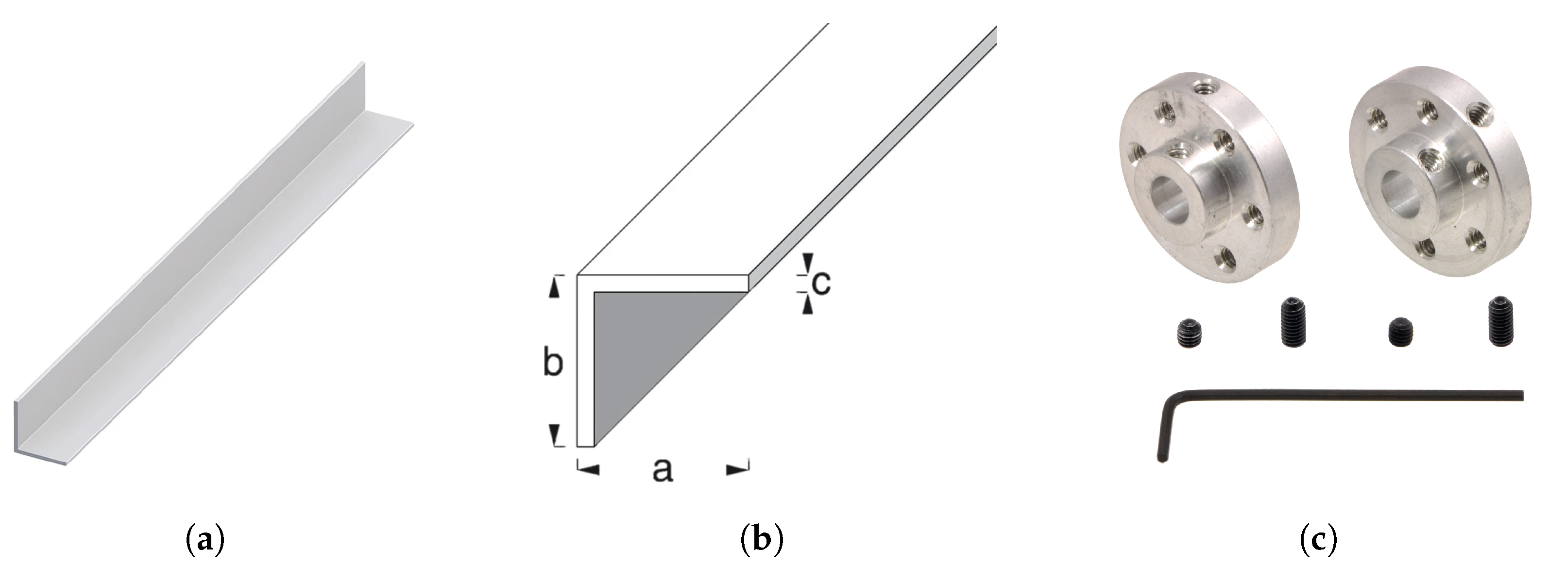
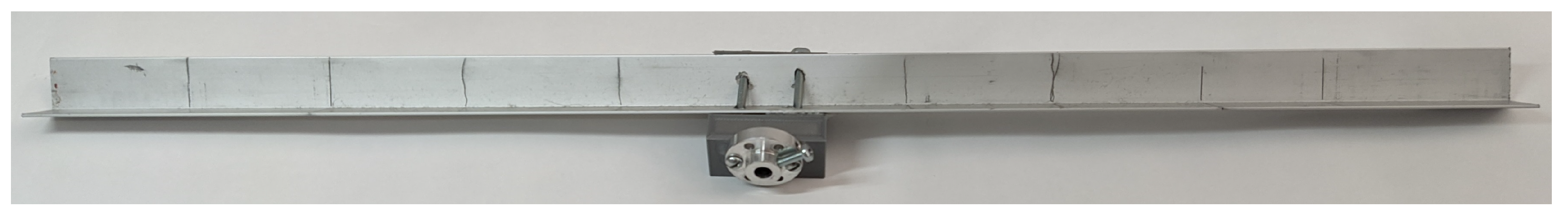
A 37D × 70L mm metal geared motor with 64 CPR Encoder from pololu was purchased for experimentation. Its main technical characteristics are nominal voltage of 12 V, maximum speed without load of 150 revolutions per minute, maximum current of 5.5 A, 4480 counts per revolution of the output shaft of the gearbox giving a transmission ratio of 70:1, and torque at maximum efficiency of 3.2 $\mathrm{k}{\mathrm{g}}_{\mathrm{f}}\mathrm{c}\mathrm{m}$. The transmission output was attached to a 50 × 2 cm aluminum rail, which is shown in Figure 1a,b using the printed part shown in Figure 1c and a Pololu Universal Aluminum Mounting Hub for 6 mm Shaft. Three-dimensional printing was used for prototyping the ball and beam braking parts as 3D printing is increasingly used in industrial applications for its high performance, rapid prototyping, and intuitive design tools [24]. Figure 2 shows the rail with the motor coupling.

Figure 1. Representation of the dimensions of the rail and coupling used. (a) View of the aluminum rail used. (b) Measurement of the aluminum used for ball and beam, where a is equal to 2 cm, b is equal to 2 cm, and c is equal to 1 mm. (c) Pololu Universal Aluminum Mounting Hub for 6 mm Shaft.

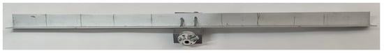
Figure 2. Final assembly of the coupling on the rail using one of the 3D-printed parts.

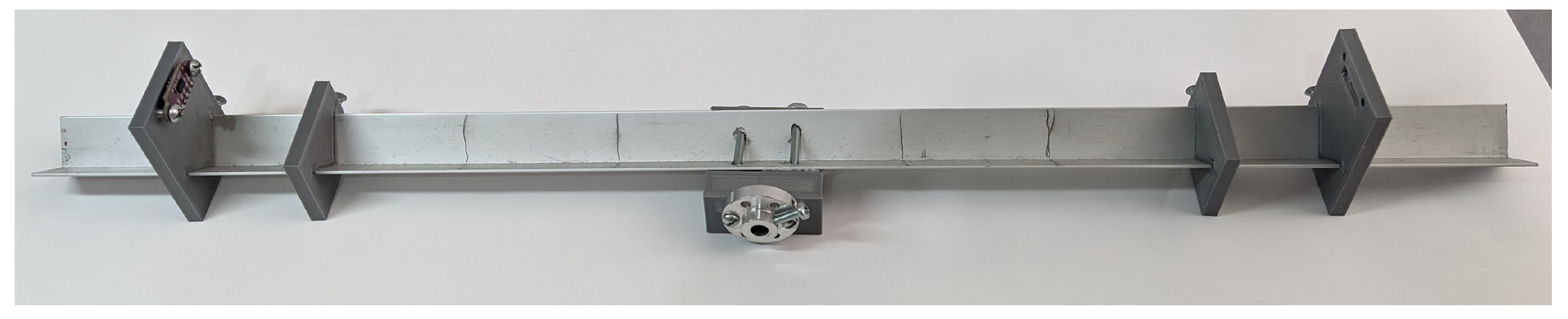
Once the rail was mounted on the aluminum cover, two plastic pieces were placed on it, which were adjusted using an M3 screw on one of its sides, serving as a physical stop for the ball moving on the rail to avoid hitting the sensor. The second piece allows for placing the vl53l0x, which is based on a time-to-flight (ToF) distance measurement system that allows for a precise measurement of the time it takes for light to travel from the closest object and return, reflected the sensor. It uses this principle to measure distances by the latest-generation infrared laser, capturing distances between 5 cm and 2 m. This sensor measures the position of the ball on the axis with respect to one of the ends. The final assembly is shown in Figure 3. The innermost rail pieces are placed 15 cm off-center on both sides to give a total length of 30 cm or 0.3 m. By comparison, the two outermost pieces are 17.5 cm off-center to eliminate distances where the sensor cannot reliably read.

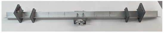
Figure 3. Final assembly of 3D-printed parts (scaffolding for the distance sensor and stopper) on the aluminum rail.

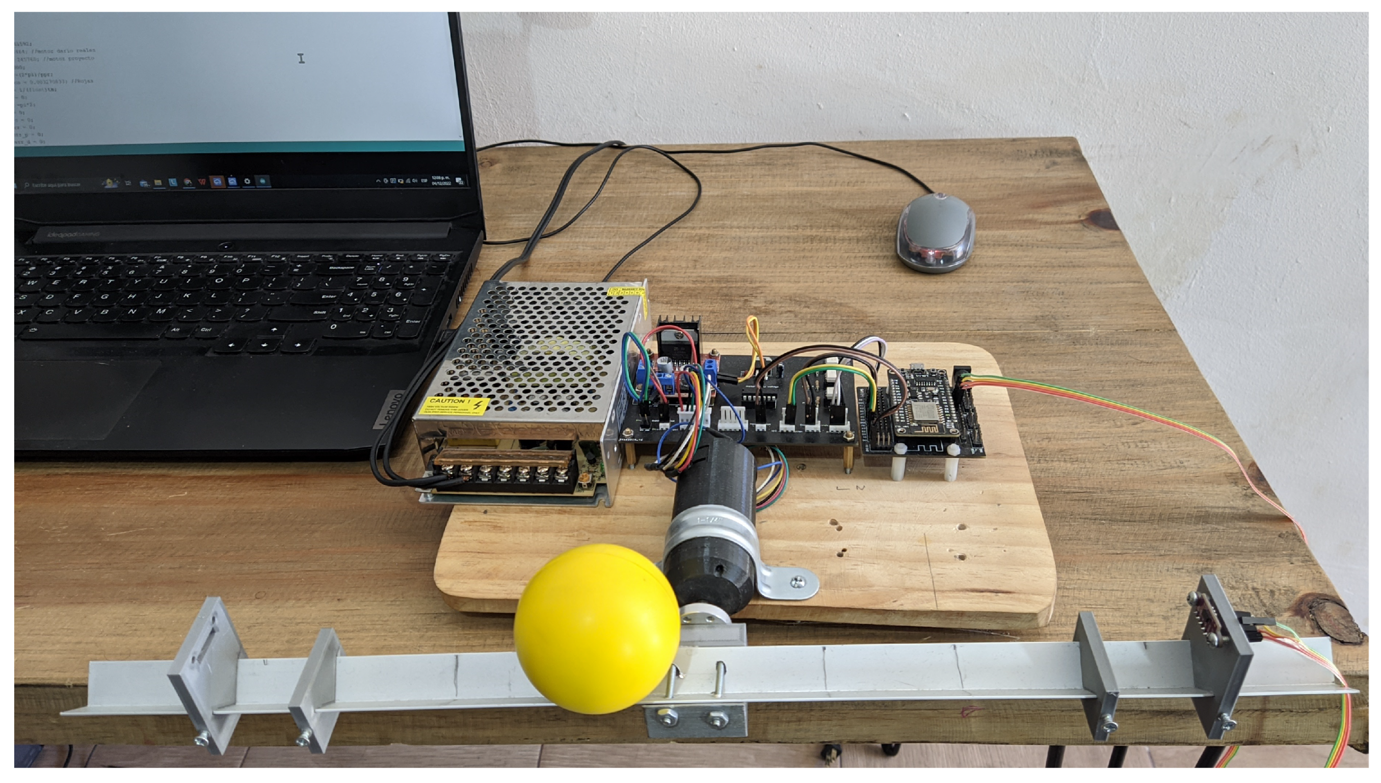
The power used for the motor was a switched source of 12 V at 10 A. The L298N H-bridge driver was used to control the direction and speed of rotation of the motor through PWM signals. The student works with the ESP8266 microcontroller (NODE MCU); however, the system implemented in this work is intended to be used with any microcontroller that has two general purpose input/output (GPIO), a PWM output, I2C communication, serial communication and two GPIO with interruption for reading the encoder. For protection of the control stage (low power) of the motor (high-power stage), 4n25 optocouplers were used. Figure 4 shows the full system.

Figure 4. Full system, including microcontroller and power electronics.

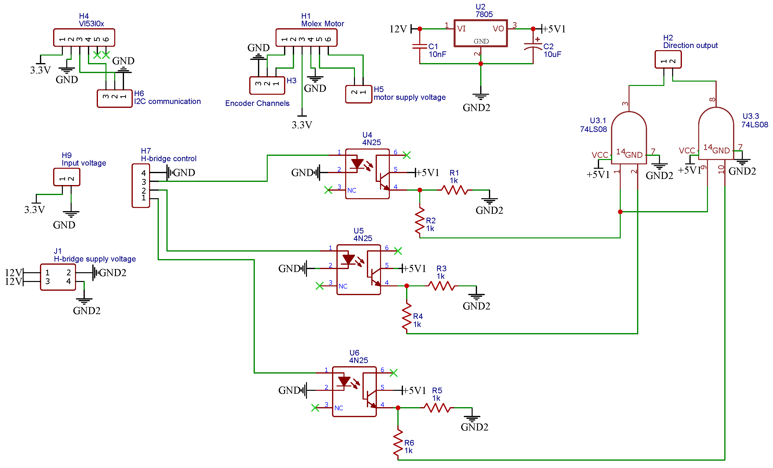
Figure 5 shows the electrical schematic of the implemented instrumentation. Inputs for the connection of the VL53L0X distance sensor named H4 are shown. There is also a connection to the microcontroller for I2C communication named H6. On the other hand, there is the H7 connection, which corresponds to the control outputs of the microcontroller towards the H bridge (L298N). These control outputs pass through the optocouplers U4, U5, and U6, which are connected to an AND gate (74LS08) to carry out the mechanical braking, which consists of sending two pulses simultaneously to both motor inputs to generate the braking. The AND gates are connected to the H2 output directed to the H-bridge input. The instrumentation card also has the H1 input corresponding to the motor input in conjunction with the encoder input (channel A, channel B, 3.3 V, and GND). H3 corresponds to the encoder reading input to the microcontroller, H5 is the H-bridge output to the motor, and H9 is the power provided by the microcontroller or an external source to the low-power elements (sensor and encoder). Finally, J1 is at the power input of the motor and the instrumentation card that, through a 7805 regulator (U2), lowers the input voltage to 5 V to power the AND gate and the optocouplers. Table 3 shows the logical truth table corresponding to the rotation of the motor, which is executed by the AND gate.

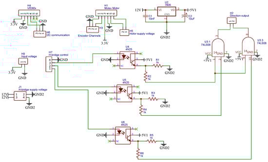
Figure 5. Development board schematic.

Table 3. Truth table of AND logic gates for motor rotation activation.

GPIO1	GPIO2	PWM	Function
DISABLE	DISABLE	DISABLE	Engine braking
DISABLE	DISABLE	ENABLE	Engine braking
DISABLE	ENABLE	DISABLE	Engine braking
DISABLE	ENABLE	ENABLE	Turn left
ENABLE	DISABLE	DISABLE	Engine braking
ENABLE	DISABLE	ENABLE	Turn right
ENABLE	ENABLE	DISABLE	Engine braking
ENABLE	ENABLE	ENABLE	Engine braking

2.2. A Dynamic Model of DC Motor

The modeling of the DC motor is given in order for the student to understand the nature of the plant. Taking into consideration the engine as an electromechanical system, the mathematical model of the DC motor is obtained by separately modeling the electrical subsystem and the mechanical subsystem. Basic concepts such as delay time, rise time, peak time, overshoot, and settlement time are explained.

A direct current motor is a machine that converts electrical energy into mechanical energy, causing a rotary movement thanks to the action of a magnetic field. It is mainly composed of two parts:

• The stator provides mechanical support and contains the poles of the machine.
• The rotor, generally cylindrical in shape, is fed with direct current through the collector formed by thin tubes. The blades are usually made of copper and are in alternating contact with the fixed brushes.

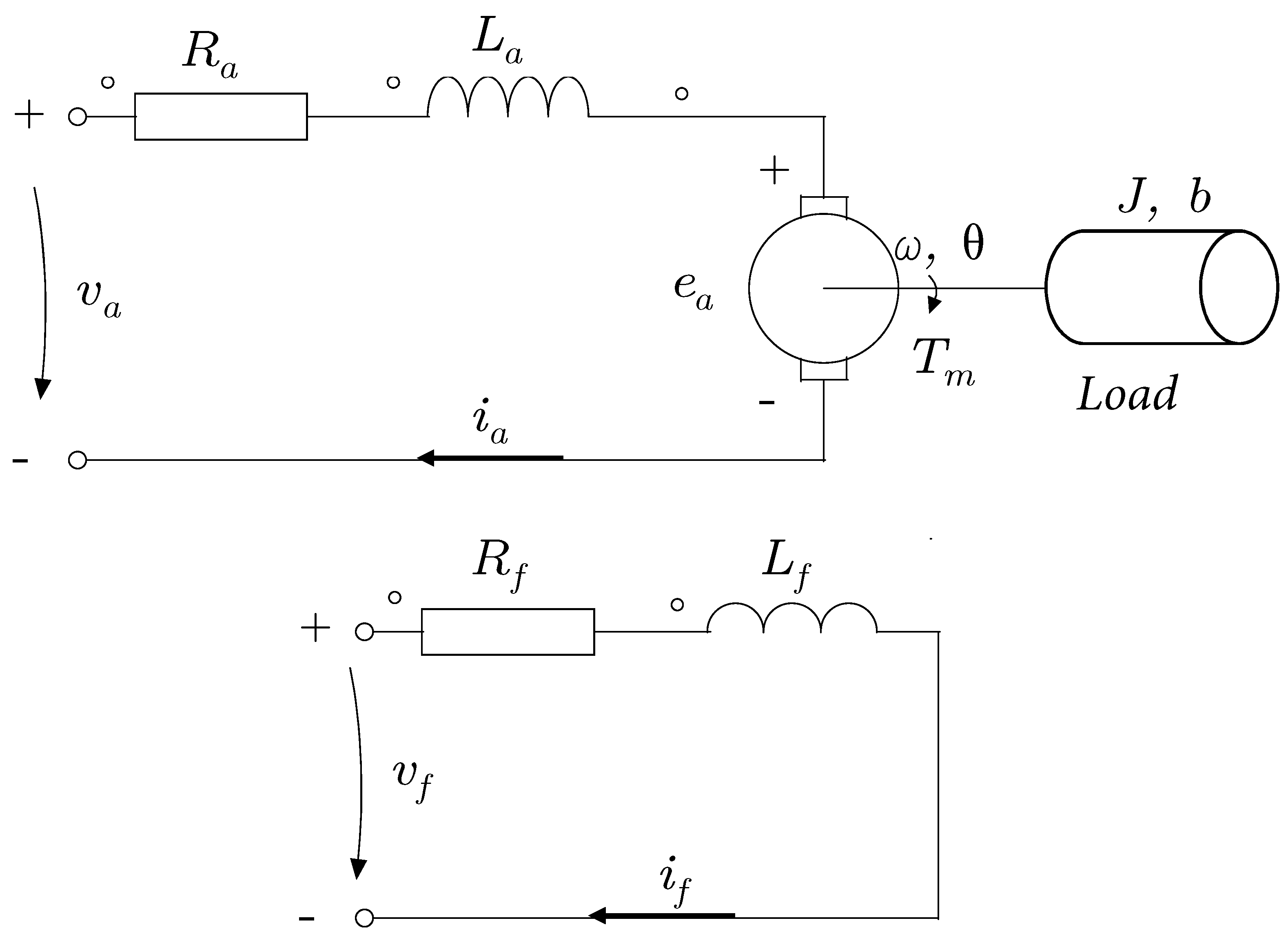
The basic operating principle of a direct current motor is explained from the case of a loop of conductive material immersed in a magnetic field, to which, a voltage is applied between its ends so that it circulates through a current. In this case, the loop constitutes the rotor of the motor, and the magnets that produce the magnetic field constitute the stator [25]. Figure 6 shows the internal wiring of the motor from an electronic point of view.

Figure 6. Internal wiring of the motor from an electronic point of view.

J is the moment of inertia referred to the motor shaft, b is the viscous friction coefficient referred to the motor shaft, $\omega$ is the angular velocity of the motor shaft, $i_a\left(t\right)$ is the armature current, $v_a\left(t\right)$ is the armature voltage, $i_f\left(t\right)$ is the field current, $v_f\left(t\right)$ is the field voltage, $T_m\left(t\right)$ is the torque developed by the motor, $L_a$ is the inductance in the armature, $R_a$ is the armature resistance, $e_a\left(t\right)$ is the counter-electromotive force, and $K_a$ and $K_m$ are constants of the motor.

The armature-controlled DC motor uses the armature current ($i_a\left(t\right)$) as the system control variable. The field in the stator is established by a permanent magnet. Obtaining the equations that describe the behavior of the system results from applying a mesh analysis on the reinforcement [26]:

$$v_a\left(t\right)=R_a{i}_a\left(t\right)+L_a\frac{d\left(i_a\left(t\right)\right)}{dt}+e_a\left(t\right)$$

(1)

where the terms shown refer to the armature of the motor and thus can be defined as: $L_a$ is the inductance, $i_a\left(t\right)$ is the current, $R_a$ is the resistance, $v_a\left(t\right)$ is the applied voltage, and $e_a\left(t\right)$ is the counter-electromotive force. Solving for the derivative remains:

$$L_a\frac{d\left(i_a\left(t\right)\right)}{dt}=v_a\left(t\right)-R_a{i}_a\left(t\right)-e_a\left(t\right)$$

(2)

Equation (3) describes the mechanical part of the motor. Solving for the derivative, Equation (4) is calculated.

$$T_m\left(t\right)=J\frac{d\left(\omega \right(t\left)\right)}{dt}+b\omega \left(t\right)$$

(3)

$$J\frac{d\left(\omega \right(t\left)\right)}{dt}=T_m\left(t\right)-b\omega \left(t\right)$$

(4)

It is assumed that there is a proportional relationship, $K_a$, between the voltage induced in the armature and the angular velocity of the motor shaft, from which, it is possible to obtain:

$$e_a\left(t\right)=K_a\omega \left(t\right)$$

(5)

In the same way, it is assumed in the mechanical part that the electro-mechanical relationship established in the torque is proportional to the electric current through $K_m$ as follows:

$$T_m\left(t\right)=K_m{i}_a\left(t\right)$$

(6)

Then, Equations (2) and (4)–(6) describe the behavior of the physical system. It is important to mention that, for many direct current motors, the armature time constant, ${\tau }_a=\frac{L_a}{R_a}$, is negligible [27]; therefore, the following transfer function is proposed, which relates the position of the motor shaft to the armature voltage:

$$\frac{\mathrm{\Theta }\left(s\right)}{V_a\left(s\right)}=\frac{K_m}{s[R_a(Js+b)+K_a{K}_m]}$$

(7)

In the specific case of the ball and beam, by adding the weight of the rail on the motor shaft, the moment of inertia J is:

$$J=n^2{J}_m+J_L$$

(8)

where $n^2$ is the ratio between the number of teeth of the gear of the motor shaft and the shaft of the rod, $J_m$ is the inertia of the motor rotor, and $J_b$ is the inertia of the rod.

Similarly, the coefficient of friction is defined as:

$$b=n^2{b}_m+b_L$$

(9)

where $b_m$ is the coefficient of friction of the motor rotor, and $J_b$ is the coefficient of friction of the rod.

The equations that relate the variables of interest to the armature stress are presented in the Laplace domain in Table 4.

Table 4. Function transfers of DC motor according to the inputs and outputs.

Relationship	Transfer Function
Electromotive force/Armature tension	$\frac{E_a\left(s\right)}{V_a\left(s\right)}=\frac{K_m{K}_a}{L_{a}J{s}^2+(R_{a}J+L_{a}b)s+R_{a}b+K_a{K}_m}$
Armature current/Armature voltage	$\frac{I_a\left(s\right)}{V_a\left(s\right)}=\frac{Js+b}{L_{a}J{s}^2+(R_{a}J+L_{a}b)s+R_{a}b+K_a{K}_m}$
Angular velocity/Armature tension	$\frac{\Omega \left(s\right)}{V_a\left(s\right)}=\frac{K_m}{L_{a}J{s}^2+(R_{a}J+L_{a}b)s+R_{a}b+K_a{K}_m}$
Armature position/tension	$\frac{\mathrm{\Theta }\left(s\right)}{V_a\left(s\right)}=\frac{K_m}{s(L_{a}J{s}^2+(R_{a}J+L_{a}b)s+R_{a}b+K_a{K}_m)}$
Motor torque/Armature tension	$\frac{T_m\left(s\right)}{V_a\left(s\right)}=\frac{K_m(sJ+b)}{L_{a}J{s}^2+(R_{a}J+L_{a}b)s+R_{a}b+K_a{K}_m}$

The objective of the experimental identification process is to obtain the mathematical model of the plant using specific inputs; for example, using a step signal. The block diagram of the closed control loop for the control of the position of the motor shaft with respect to the voting is shown in Figure 7. The mathematical model used for identification is presented below [28]:

$$\frac{\mathrm{\Theta }\left(s\right)}{V_a\left(s\right)}=\frac{C_k}{s(s+C_p)}$$

(10)

where $C_k=\frac{K_m}{R_{a}J}$ y $C_p=\frac{R_{a}b+K_m{K}_a}{R_{a}J}$.

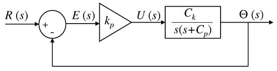
Figure 7. Closed loop DC motor proportional control block diagram.

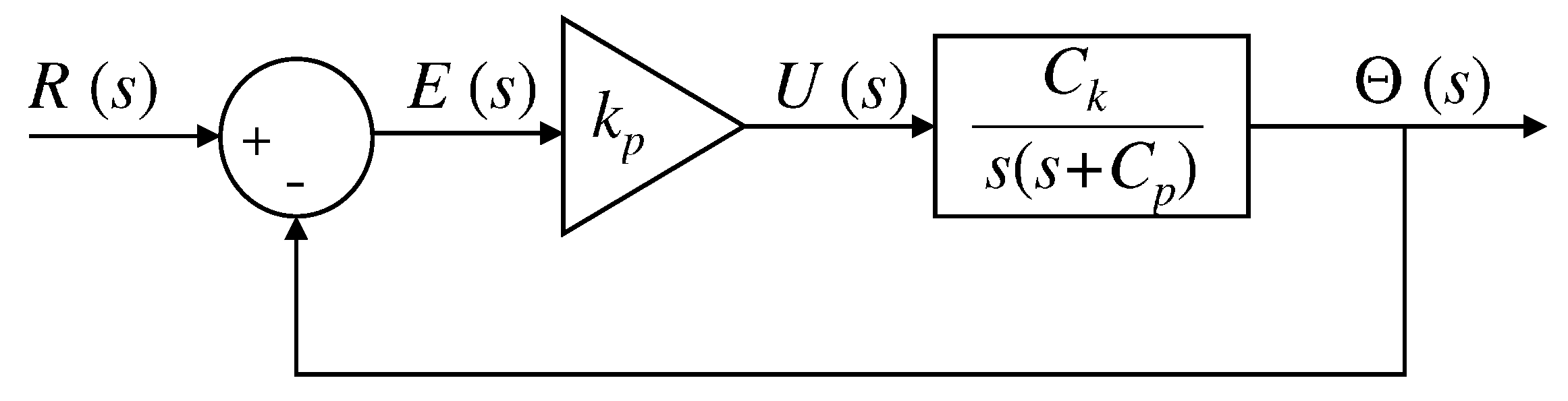
Proportional control is used to find the parameters that define the plant. The block diagram of the proposed system is presented in the following figure:

The closed-loop transfer function of the presented block diagram is shown in Equation  (11).

$$\frac{\mathrm{\Theta }\left(s\right)}{V_a\left(s\right)}=\frac{\frac{K_p{C}_k}{s(s+C_p)}}{1+\frac{K_p{C}_k}{s(s+C_p)}}=\frac{k_p{C}_k}{s^2+C_{p}s+k_p{C}_k}$$

(11)

The objective of the procedure is to increase the proportional constant $k_p$ until obtaining an underdamped response. After performing the process, it is expected that the response of the model has a behavior similar to that presented in Figure 8.

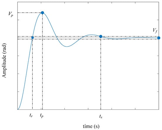
Figure 8. Closed loop response of motor shaft position with proportional control.

$t_r$ is the time elapsed until the system reaches its final value for the first time, $t_p$ is the time required for the response to obtain the first peak of the overshoot, $t_s$ is the time needed for the curve response rate to reach and stay within a range near the final value, which is usually within 2% or 5%, and $V_f$ is the final value of the system response. Finally, $V_p$ is the value of the first overshoot. At this point, the equations of the plant parameters are defined. When performing the recognition of the variables, it is observed that it is a second-order system, and it is possible to propose [29,30]:

$$\frac{k_p{C}_k}{s^2+C_{p}s+k_p{C}_k}=\frac{{{\omega }_n}^2}{s^2+2\zeta {{\omega }_n}^{2}s+{{\omega }_n}^2}$$

(12)

From Equation (12), the following is used:

$$C_p=2\zeta {\omega }_n$$

(13)

$${{\omega }_n}^2=k_p{C}_k$$

(14)

From Equation (14), it is obtained that:

$$C_k=\frac{{{\omega }_n}^2}{k_p}$$

(15)

Once the relationships of the constants that describe the engine model have been found, it is possible to calculate them, considering the maximum overshoot $M_p$, which is the magnitude of the first overshoot that occurs in the peak time measured from the reference signal.

$$M_p=100e^{\frac{\zeta \pi }{\sqrt{1-{\zeta }^2}}}=\frac{c\left(t_p\right)-c(\infty )}{c(\infty )}$$

(16)

$c\left(t_p\right)$ is the output value of the system at peak time and $c(\infty )$ is the output value of the steady state system.

Applying the natural logarithm in Equation (16), it is obtained that:

$$Ln\left(\frac{M_p}{100}\right)=\frac{\zeta \pi }{\sqrt{1-{\zeta }^2}}$$

(17)

From Equation (17), it is obtained that:

$$\zeta =\frac{|Ln\left(\frac{M_p}{100}\right)|}{\sqrt{{\left(Ln\left(\frac{M_p}{100}\right)\right)}^2+{\pi }^2}}$$

(18)

For an underdamped system, the rise time ($t_r$) is defined as:

$$t_r=\frac{1}{{\omega }_d}{tan}^{-1}\left(\frac{{\omega }_d}{-\sigma }\right)=\frac{\pi -\beta }{{\omega }_d}$$

(19)

$\beta ={tan}^{-1}\left(\frac{{\omega }_d}{-\sigma }\right)$, $\sigma =\zeta {\omega }_n$ y ${\omega }_d={\omega }_n\sqrt{1-{\zeta }^2}$ is called the damped oscillation frequency.

From Equation (19), it is obtained that:

$${\omega }_d=\frac{1}{t_r}{tan}^{-1}\left(\pi -\frac{\sqrt{1-{\zeta }^2}}{\zeta }\right)$$

(20)

Finally, ${\omega }_n$ is calculated from the following relation:

$${\omega }_n=\frac{{\omega }_d}{\sqrt{1-{\zeta }^2}}$$

(21)

Once ${\omega }_n$ and $\zeta$ have been calculated, it is possible to find the constants that describe the behavior of the engine, $C_k$ and $C_p$.

Proposal for DC Motor Identification

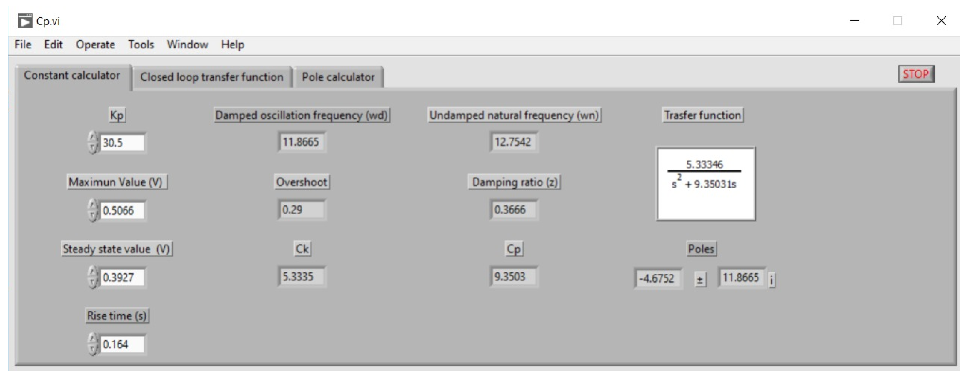
In order to facilitate the previously detailed calculations of developing an application in LabVIEW, which was ported to an installable file so that it can be used on any computer without having LabVIEW installed, the developed interface is shown in Figure 9.

Figure 9. Graphical interface of the DC motor constants calculator.

The motor identification was performed using a reference of $Ref=\frac{\pi }{8}$ rad, and a supply voltage of V = 12 V using the next equation, $K_p$, is defined:

$$K_p=\frac{V}{Ref}=30.5$$

(22)

After performing the experiment under these conditions, the values were $c\left(t_p\right)=0.5066$ rad, $c(\infty )=0.3927$ rad, and $t_r=0.164\mathrm{s}$. According to the values given by the developed calculator, the values obtained for $C_k$ and $C_p$ are 5.33 and 9.35, respectively. Then, using these values along with Equation (10) results in the transfer function that describes the system:

$$\frac{\mathrm{\Theta }\left(s\right)}{V_a\left(s\right)}=\frac{5.333}{s(s+9.35)}$$

(23)

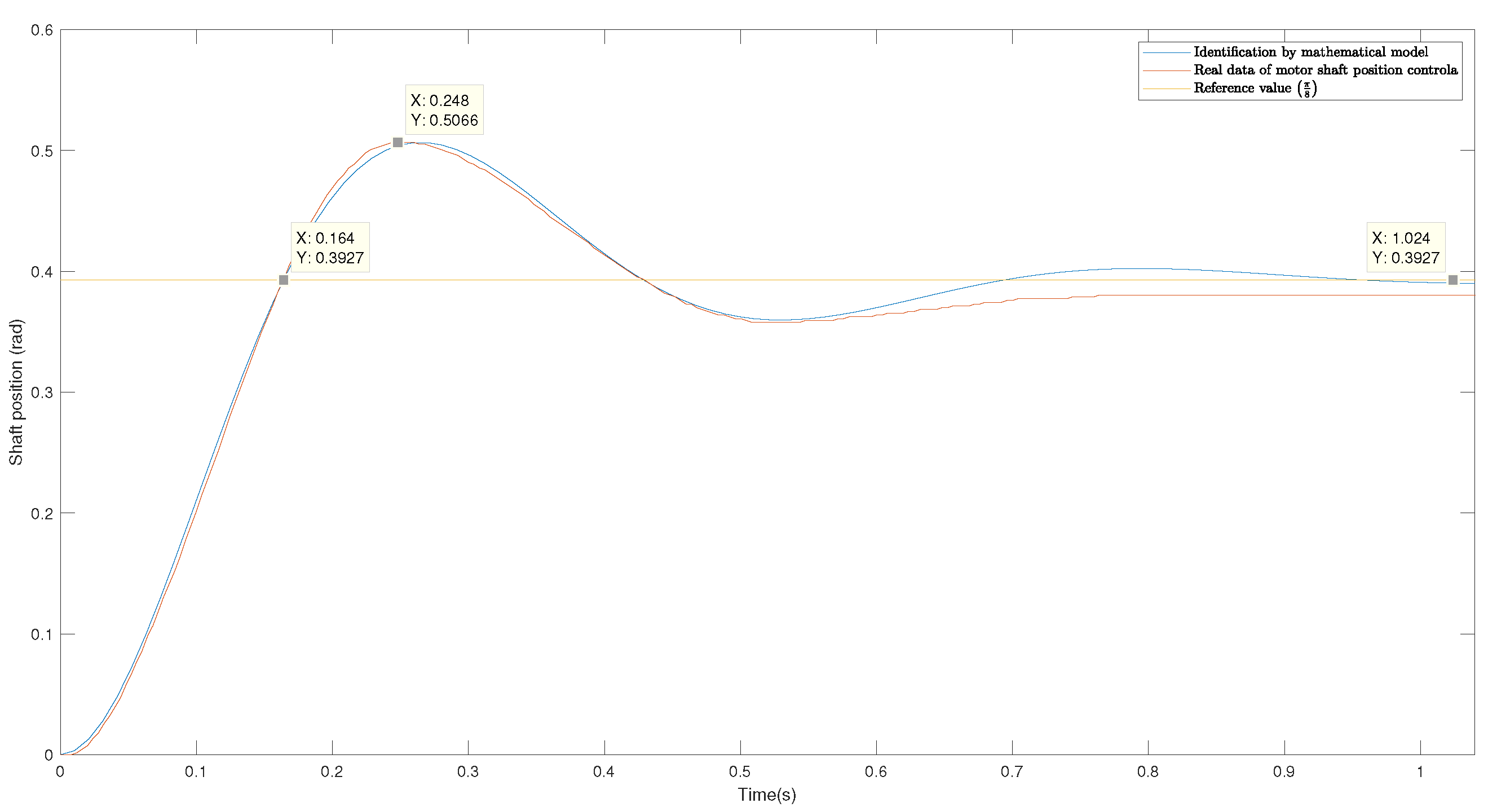
Figure 10 compares the mathematical model obtained against the data of the proportional control of the motor shaft. It is observed that both the uphill and downhill slopes are almost identical between the two graphs. However, a slight gap is shown. This may be due to the non-linearities of the motor, which are not considered within the model. It should be noted that the identification presented is made with the rail attached to the motor shaft.

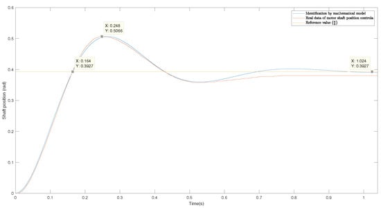
Figure 10. Comparison of the mathematical model obtained against the data of the proportional control of the motor shaft.

2.3. A Dynamic Model of Ball and Beam

The ball and beam system is a famous educational prototype in system control. When considering the complete model of the mechanism, it is discovered that it is non-linear and difficult to control due to the centrifugal force generated by the rotation of the rod. However, this phenomenon is relevant only when the speed of the rod is very high. Other non-linearities may be caused by different sources of friction; for example, the inner friction of the actuator, which can be taken into account when estimating the mathematical model that describes it, or the aerodynamic drag on the ball, which only becomes relevant when it is moving at high speeds. If it is assumed that the rod and ball move at low velocities and that the rod only describes angles close to the horizontal, then the model is linear and is a good test bed for classical control techniques. Figure 11 shows a simplified representation of the physical dynamics of the ball and beam [30].

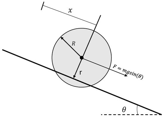
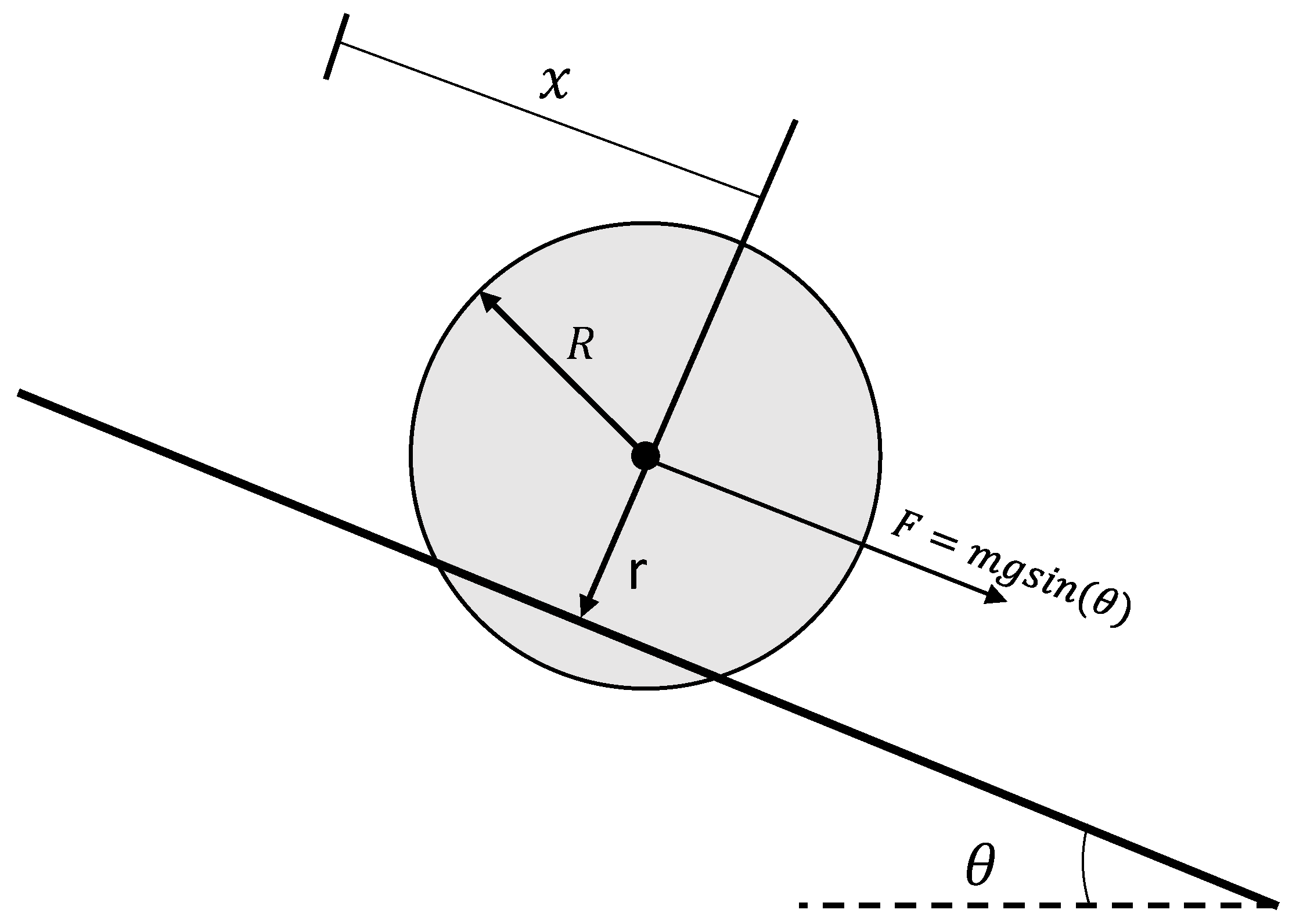
Figure 11. Ball and beam system, where x is the position of the ball measured from the left end of the rail, $\theta$ is the inclination of the rail with respect to the horizontal, and R and r represent, respectively, the radius of the ball (spherical) and the radius of gyration of the ball about the edges of the channel.

The connection of the rod with the motor is modeled in the same way as in Section 2.2 since, in this specific situation, the rod performs the function of the load on the shaft. On the other hand, the following procedure is carried out to model the fall of the ball on the rail.

It is assumed that the inclination $\theta$ of the rod produces any displacement x of the ball. The sought mathematical model is obtained by applying Newton’s second law to describe the translational motion of the ball, which has two components: (1) the translational motion of a particle with mass m and (2) the rotational motion about its axis of a sphere with mass m [30,31,32].

Initially, the ball is stationary, and turning the rail causes, due to friction, the ball to rotate (without changing its position in space). If $\omega$ is the angular velocity with which the ball rotates and v is the velocity with which the channel slides to the left, then:

$$\omega \times r=v$$

(24)

where × signifies the cross product of two vectors. By leveraging the fact that the angular velocity and the radius are perpendicular, the expression can be written in terms of the magnitudes of the vectors involved as:

$$\omega r=v$$

(25)

$$\dot{\omega }r={\displaystyle \frac{\dot{v}}{r}}$$

(26)

Let f be the force that the channel exerts on the ball and that causes it to rotate. Note that this force is applied at a distance r from the center of the ball. Then, rf is the torque exerted by the channel on the ball. Applying Newton’s second law to this situation, we obtain:

$$J_b\dot{\omega }=fr$$

(27)

$$f={\displaystyle \frac{2}{5}}m\dot{v}{\displaystyle \frac{R^2}{r^2}}$$

(28)

where $J_b={\displaystyle \frac{2}{5}}m{R}^2$, and is the inertia of a solid sphere of mass m and radius R that rotates on its own axis (ball).

Now the ball starts to move, and the channel remains at rest, so its position x now changes and the velocity and acceleration of the ball are given as (assume that the ball rolls over the edges of the channel without skidding):

$$\dot{x}=-v,\ddot{x}=-\dot{v}$$

(29)

Then, f is the equivalent force that the rotating movement of the ball exerts on itself, contributing to its displacement along the channel. With this background, Newton’s second law can be applied to the translational motion of the pellet, considering that, in addition to the effect of gravity, there is a force f that the rotation of the pellet exerts on itself:

$$m\ddot{x}=f+mgsin\left(\theta \right)$$

(30)

Therefore, using the previous definitions of Equations (28) and (29), we obtain:

$$m\ddot{x}=-{\displaystyle \frac{2}{5}}m\ddot{x}{\displaystyle \frac{R^2}{r^2}}+mgsin\left(\theta \right)$$

(31)

where g is the constant of gravity.

After simplifying the above equation, the following is obtained:

$$\left(1+{\displaystyle \frac{2}{5}}{\displaystyle \frac{R^2}{r^2}}\right)\ddot{x}=gsin\left(\theta \right)$$

(32)

As mentioned at the beginning, it was taken into account that $\theta$ will take values close to 0; therefore, the following consideration can be made:

$$sin\left(\theta \right)\approx \theta$$

(33)

Therefore, Equation (32) is considered as follows:

$$\left(1+{\displaystyle \frac{2}{5}}{\displaystyle \frac{R^2}{r^2}}\right)\ddot{x}=g\theta$$

(34)

By applying the Laplace transform with the initial values equal to 0, the following expression is obtained:

$${\displaystyle \frac{X\left(s\right)}{\theta \left(s\right)}}={\displaystyle \frac{c}{s^2}}$$

(35)

where c is defined as

$$c={\displaystyle \frac{g}{1+{\displaystyle \frac{2}{5}}{\displaystyle \frac{R^2}{r^2}}}}$$

(36)

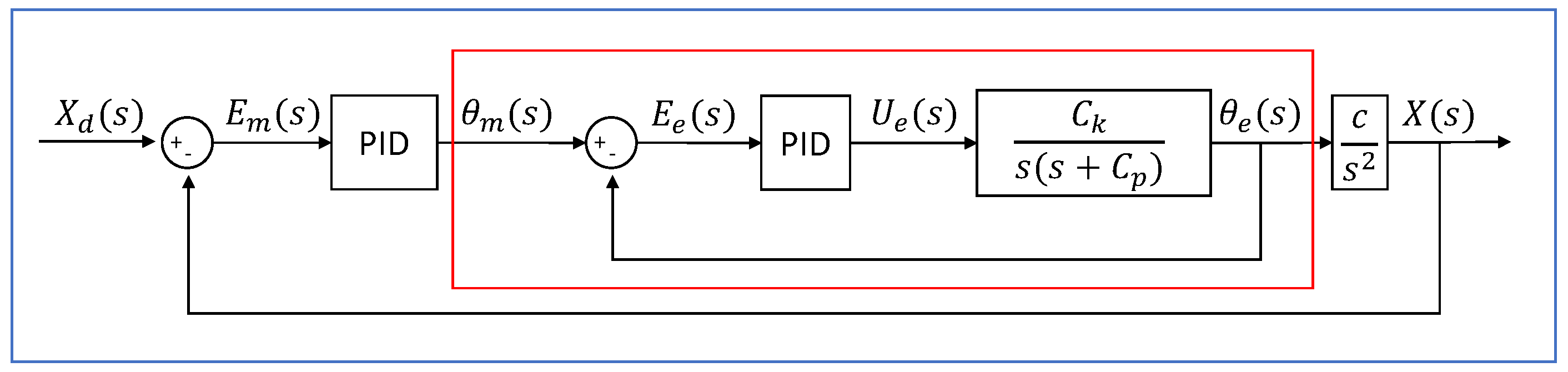
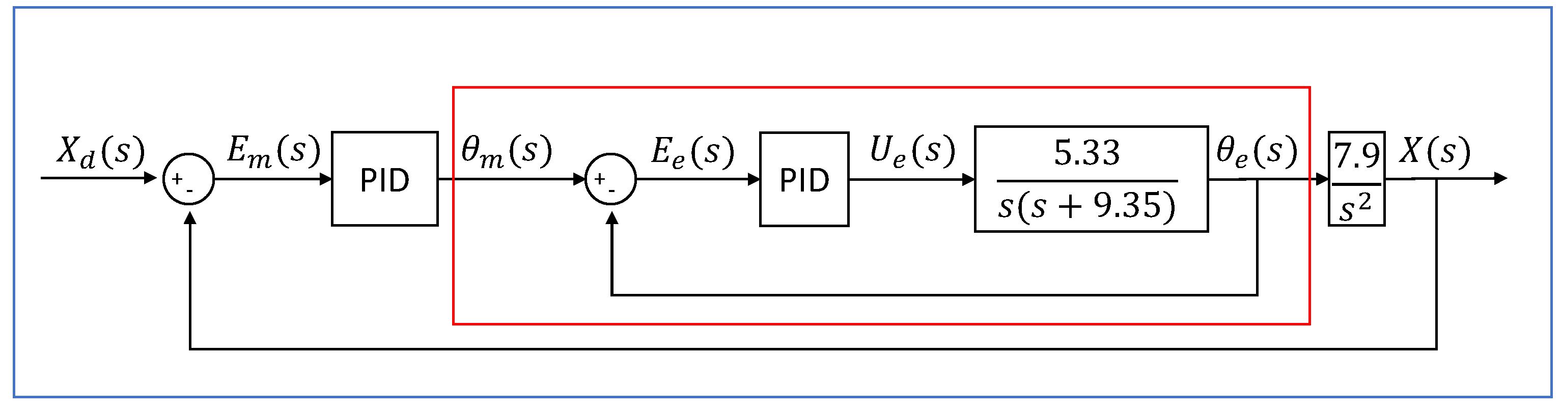
Figure 12 shows the block diagram of the control loops to be implemented in the ball and beam. It is a system in which the position of a sphere on a bar or rail is controlled by modifying its inclination. Due to gravity, the rotation of the sphere is confined to the channel located on the upper face of the bar [30].

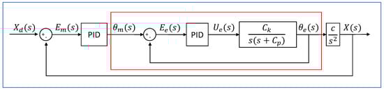
Figure 12. Ball and beam system block diagram. The blue box encloses the master control loop, whereas the red has the slave control loop.

$X_d\left(s\right)$ is the desired position of the ball over the rail, $X\left(s\right)$ is the actual position of the ball, $E_m\left(s\right)$ is the error between the desired position and the current position of the ball, $E_e\left(s\right)$ is the error in between the desired position of the motor shaft and the actual position of the motor shaft, ${\mathrm{\Theta }}_m\left(s\right)$ is the reference angular position, ${\mathrm{\Theta }}_e\left(s\right)$ is the output angular position of the slave loop, $U_e\left(s\right)$ is the control effort of the controller slave, and c is the motion constant of the ball [30].

The length of the rail presented in this work is 0.3 m. It is defined that position 0 is located in the center of the rail, whereas positions −0.15 m and 0.15 m are located at each end. The constant c is obtained in the following way. The motor shaft angle is set to a known value. The ball is placed at the end of the sensor (−0.15 m) and dropped until it reaches a value of 0.15 m. Subsequently, using Equation (37), the value of c closest to the graph made from the measurement values is proposed. It is essential to mention that the values obtained by the sensor must be restored to the initial value obtained in order to obtain the distance traveled by the ball in time t [30].

$$\frac{c{\mathrm{\Theta }}_0{t}^2}{2}$$

(37)

where $\mathrm{\Theta }$ is the initial angle of the rail, t is the sampling time of the sensor, and c is the parameter of the fall of the ball on the rail.

Proposal for Ball and Beam Identification

The first step is to calibrate the sensor since the output given by the vl53l0x is an integer value in mm that takes the sensor as a reference of zero. Due to this and because it is necessary to place reference zero in the middle of the rail, it is necessary to conduct a linearization of the sensor values according to our needs. Three measurements are taken at distances of 0 m, 0.05 m, 0.1 m, −0.05 m, and −0.1 m. With the values obtained, the linear regression calculation is applied to obtain the equation of a straight line that allows us to calculate the distance from sensor data. Table 5 shows an example of data acquisition to obtain the equation of the line.The equation of the resulting line is shown in Equation (38), where x is the value given by the distance sensor and y is the position of the ball on the rail [30].

$$y=-0.0009x+0.1822$$

(38)

Table 5. Values for position sensor calibration.

Sensor Values	Position of the Ball on the Rail
329 mm	−0.1 m
267 mm	−0.05 m
217 mm	0 m
154 mm	0.05 m
96 mm	0.1 m
336 mm	−0.1 m
265 mm	−0.05 m
212 mm	0 m
152 mm	0.05 m
96 mm	0.1 m
327 mm	−0.1 m
262 mm	−0.05 m
217 mm	0 m
158 mm	0.05 m
94 mm	0.1 m

The linear relationship between the variables x and y was evaluated using the coefficient of determination or $R^2$ since an accurate reading of the position of the ball is crucial. As a result, $R^2=0.997$ was obtained, indicating a very reliable model for future forecasts.

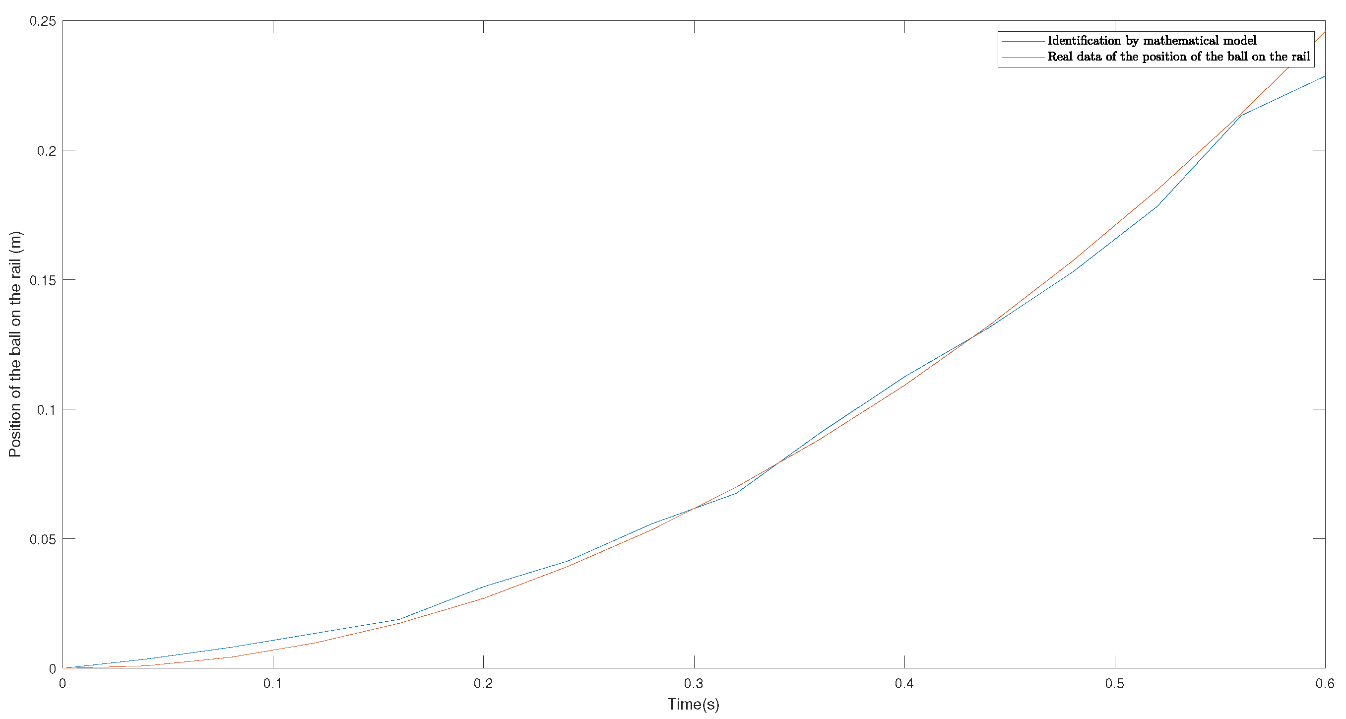
Once the calibration was performed, the value c was calculated for the identification of the fall of the ball on the rail. For the identification of c, an angle of 0.17 radians or 10 degrees was selected, and there was a sampling frequency of 0.04 s (40 ms) because the position sensor vl53l0x has a maximum response speed of 0.033 s (33 ms) [33]. As mentioned in the previous section, the ball was dropped on the rail starting from the sensor, and the resulting graph was compared with that given by Equation (38). Figure 13 shows the result of the experimental part and the mathematical modeling with $c=7.46$. For the experimentation, a 60 mm diameter polyurethane foam ball was used.

Figure 13. Mathematical model of the dynamics of the fall of the ball in comparison with the natural dynamics of the fall.

The value of c was calculated by performing a nonlinear regression using the method of least squares, which aims to minimize the sum of squares of the error between the given function (37) and the real values. The value of $R_2$ obtained is 0.991.

Figure 14 shows the ball and beam control block diagram in a closed loop, with the plant constants identified; thus, the next step is to tune the PID controllers.

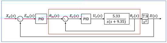
Figure 14. The block diagram of the ball and beam control in closed loop, with the plant constants identified.

2.4. PID Controller

A controller compares the actual value of the output of a plant with the desired value, calculates the error between both variables, and produces a control signal that reduces the error to zero or a negligible value [34,35].

Proportional control action: The control action of a proportional controller is the relationship between the output of the system $y\left(t\right)$ and the error $e\left(t\right)$. This relationship is defined in Equation (39).

$$y\left(t\right)=K_{p}e\left(t\right)$$

(39)

The transfer function of the proportional control in the Laplace space is defined in Equation (40). $K_p$ is considered as the proportional gain.

$$\frac{Y\left(s\right)}{E\left(s\right)}=K_p$$

(40)

Integral control action: This control action, as its name indicates, calculates the integral of the error signal $e\left(t\right)$ as shown in Equation (41).

$$y\left(t\right)=K_i{\int }_0^{t}e\left(t\right)dt$$

(41)

The transfer function of the integral control in the Laplace space is defined in Equation (42). $K_i$ is considered the integral gain.

$$\frac{Y\left(s\right)}{E\left(s\right)}=\frac{K_i}{s}$$

(42)

Derivative control action: This control action is proportional to the derivative of the error signal $e\left(t\right)$. The derivative of the error is another way of calling the “speed” of the error. Its equation as a function of time is shown in (43).

$$y\left(t\right)=K_d\frac{d\left(e\right(t\left)\right)}{dt}$$

(43)

The transfer function of the derivative control in the Laplace space is defined in Equation (44). $K_d$ is considered as the derivative gain.

$$\frac{Y\left(s\right)}{E\left(s\right)}=K_{d}s$$

(44)

Proportional-integral-derivative control action: The sum of the proportional, integral, and derivative control action is called PID control action. The equation that defines this controller is given by Equation (45).

$$y\left(t\right)=K_{p}e\left(t\right)+K_i{\int }_0^{t}e\left(t\right)dt+K_d\frac{d\left(e\right(t\left)\right)}{dt}$$

(45)

The transfer function of a PID controller is given by Equation (46).

$$\frac{Y\left(s\right)}{E\left(s\right)}=K_p+\frac{K_i}{s}+K_{d}s$$

(46)

Algorithm 1 shows a pseudocode of the PID controller implementation for motor shaft position control.

Algorithm 1 PID control pseudocode for motor shaft position.

Define the desired position of the motor shaft ($DP$)  Define sampling time ($t_s$)  Define $K_p$, $K_d$, $K_i$  previous error = 0  integral error = 0  while (1) do        if sampling time passed then            Calculate the current position of the motor shaft (P)            $error=DP-P$            $derivativeerror={\displaystyle \frac{error-previouserror}{t_s}}$            $integralerror=(integralerror+error)\ast t_s$            $output=Kp\ast error+Kd\ast derivativeerror+Ki\ast integralerror$            $previouserror=error$        end if  end while

Proposal for PID Controller Tuning

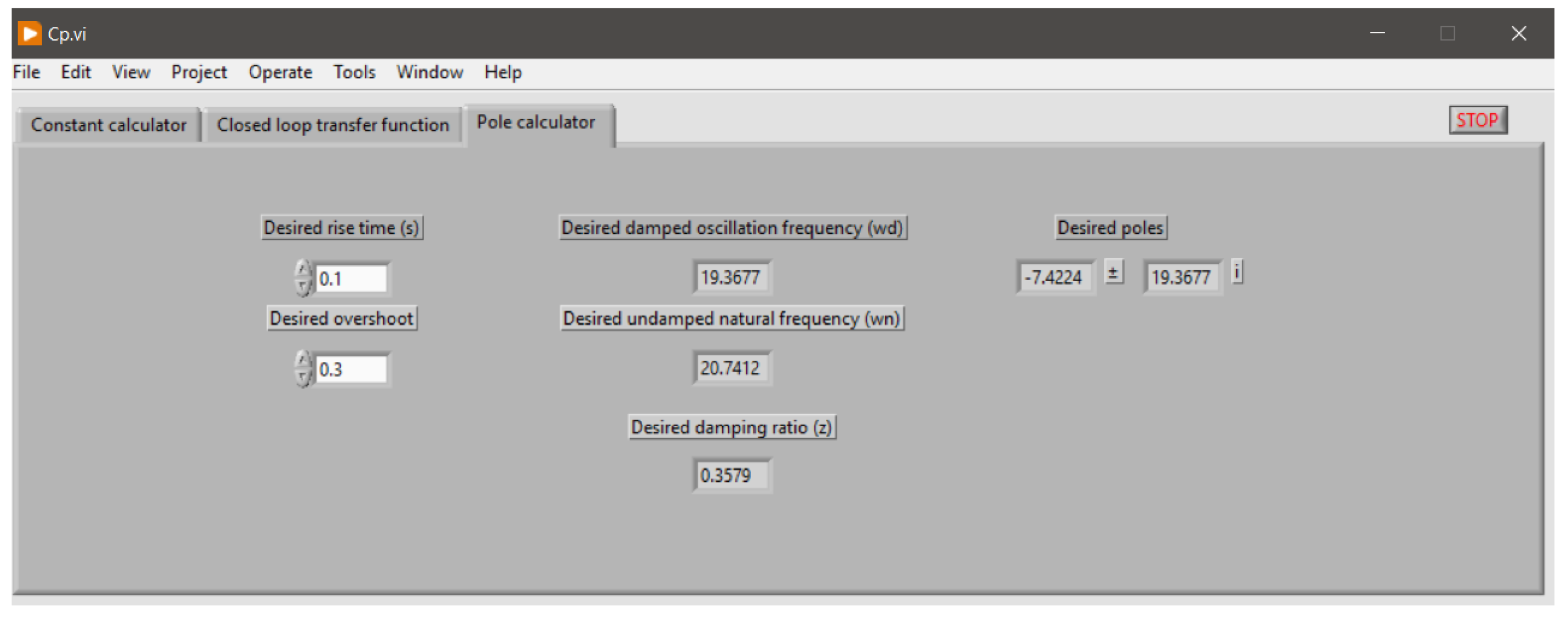
After having obtained the model of the plant, the proportional-derivative controller of the slave loop was adjusted, which is shown in Figure 15. This adjustment was made using the MatLab Sisotool tool. It must be considered that the design requirements are $t_r$ = 0.1 s and $M_p$ = 30% as the maximum values. For this, the root locus method was used, which bases its operation on varying a gain from 0 to ∞ [36]. In order for the system response to meet the requirements of the rise time and overshoot, the poles in the system’s closed loop must be $-7.422\pm 19.3677i$. The graphical interface shown in Figure 16 was used to calculate the desired poles. It is essential to highlight that the calculator only allows us to calculate the necessary poles to comply with the DC motor control instructions.

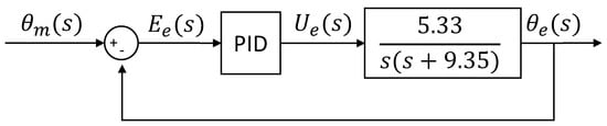
Figure 15. Slave control loop block diagram.

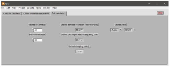
Figure 16. Graphical interface for calculating the desired poles for the use of the locus of roots.

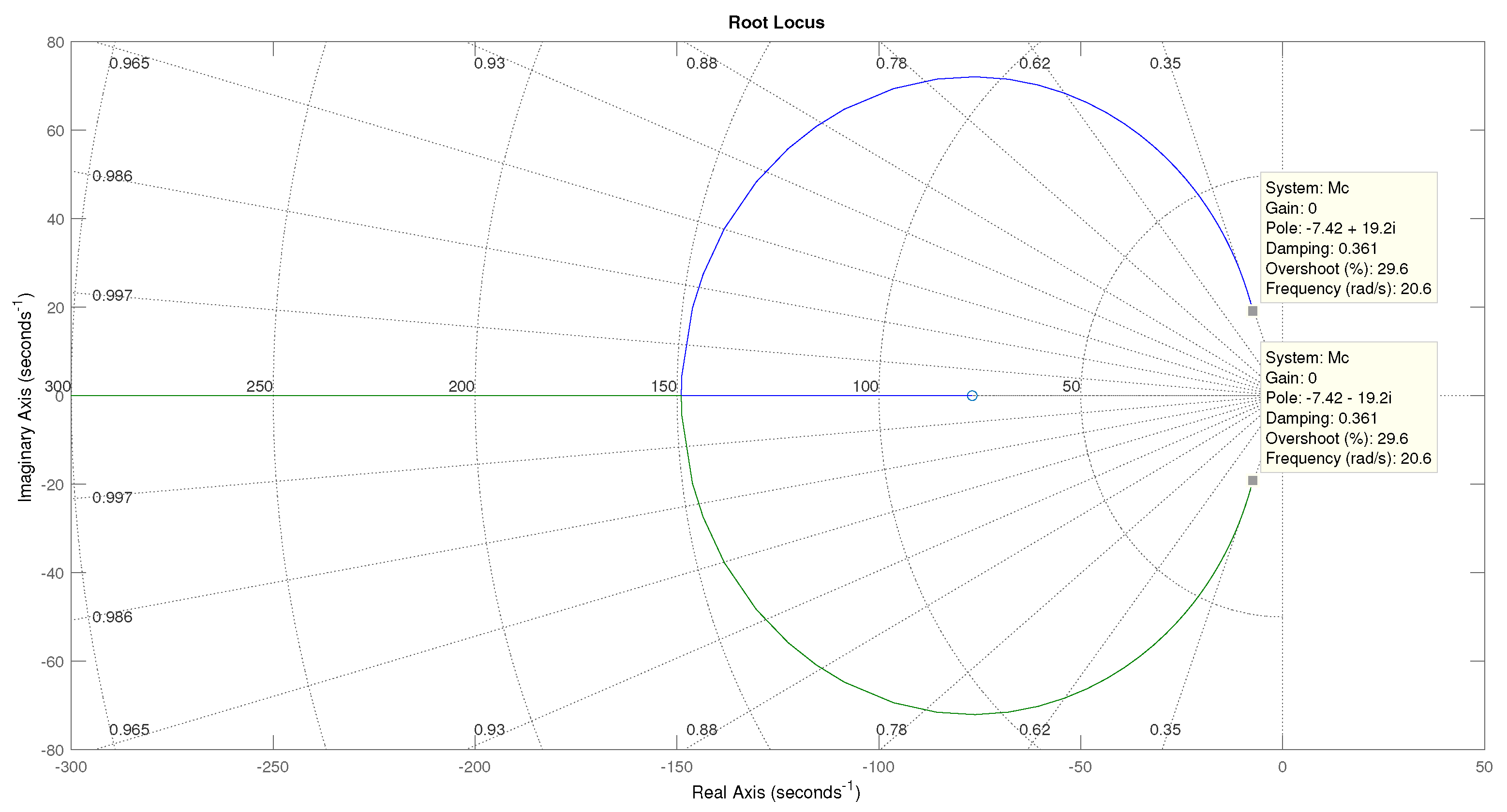
Figure 17 shows the locus of the roots for the motor implemented throughout this proposal. According to the results given by Sisotool, to reach these poles in a closed loop, a $K_p$ = 79.2 and a $K_d$ = 1.03 are necessary. Figure 18a shows the block diagram with the PID controller values, and Figure 18b shows the block diagram after the reduction, resulting in a single transfer function.

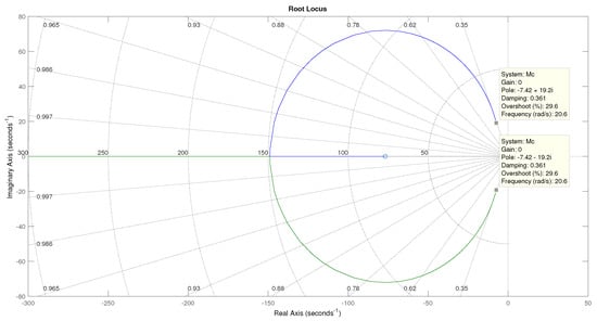
Figure 17. Locus of roots for the transfer function of a DC motor.

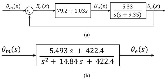
Figure 18. Graphs resulting from (a) position control of the slave loop motor axis and (b) control voltage resulting from the calculated PD.

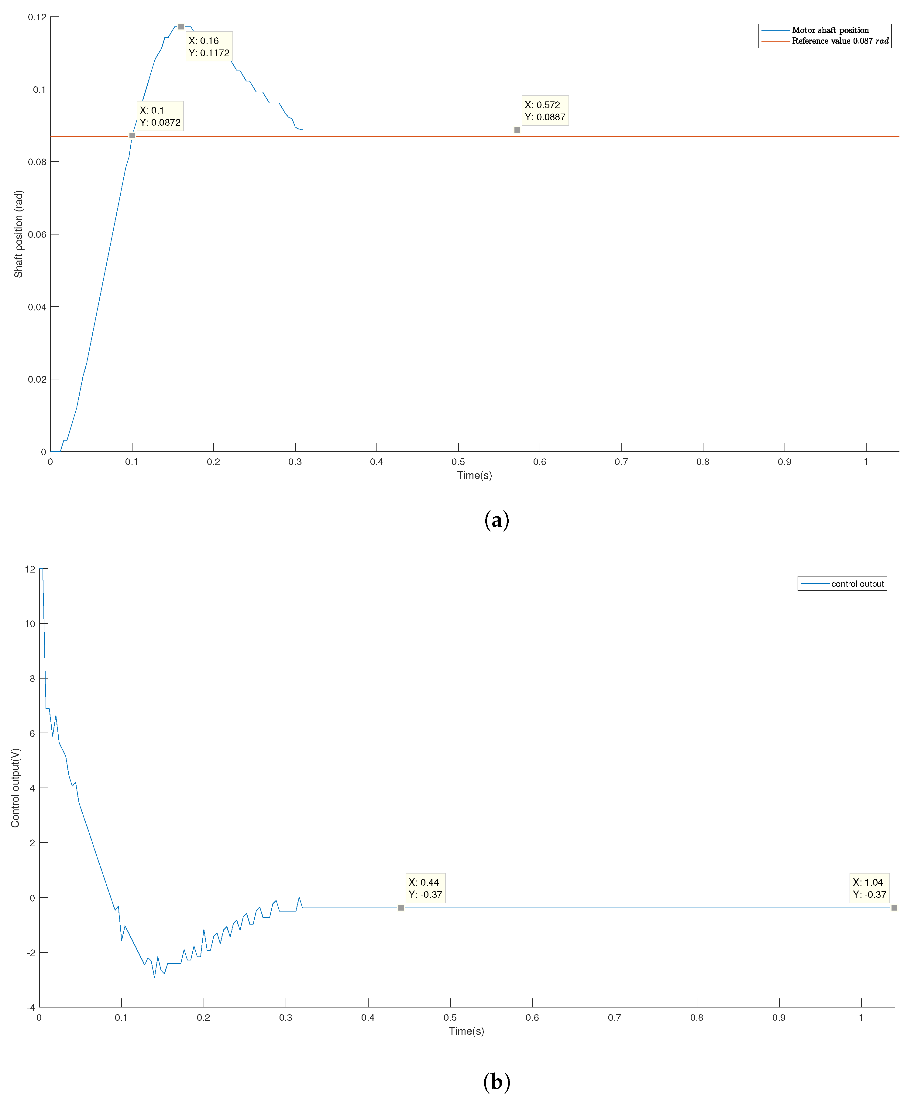
Figure 19a shows the response of the motor shaft in a closed loop applying the PD controller. It can be seen that it does not arrive even though the voltage signal shown in Figure 19b is 0.37. However, the motor being implemented begins its movement from 0.8 V. This non-linearity is not simulated in the given transfer function, so it must be considered, if necessary, through the fine adjustment of the control variables. On the other hand, it is observed that there is an overshoot of 34.7% and a rise time of 0.1 s. This additional overshoot is due, as mentioned above, to non-linearities present in the motor.

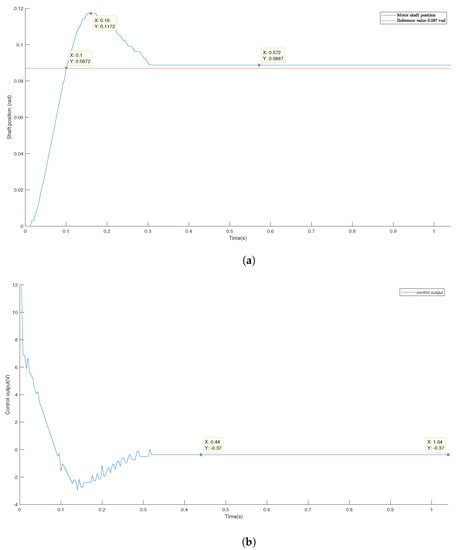
Figure 19. (a) Block diagram with the values of the PID controller; (b) block diagram after the reduction in the block diagram.

Once the slave loop is finished, the master loop is tuned. For this, a PD control is used. The first step is to perform the diagram reduction shown in Figure 14, which results in the block diagram of Figure 20.

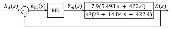
Figure 20. Reduced master loop block diagram.

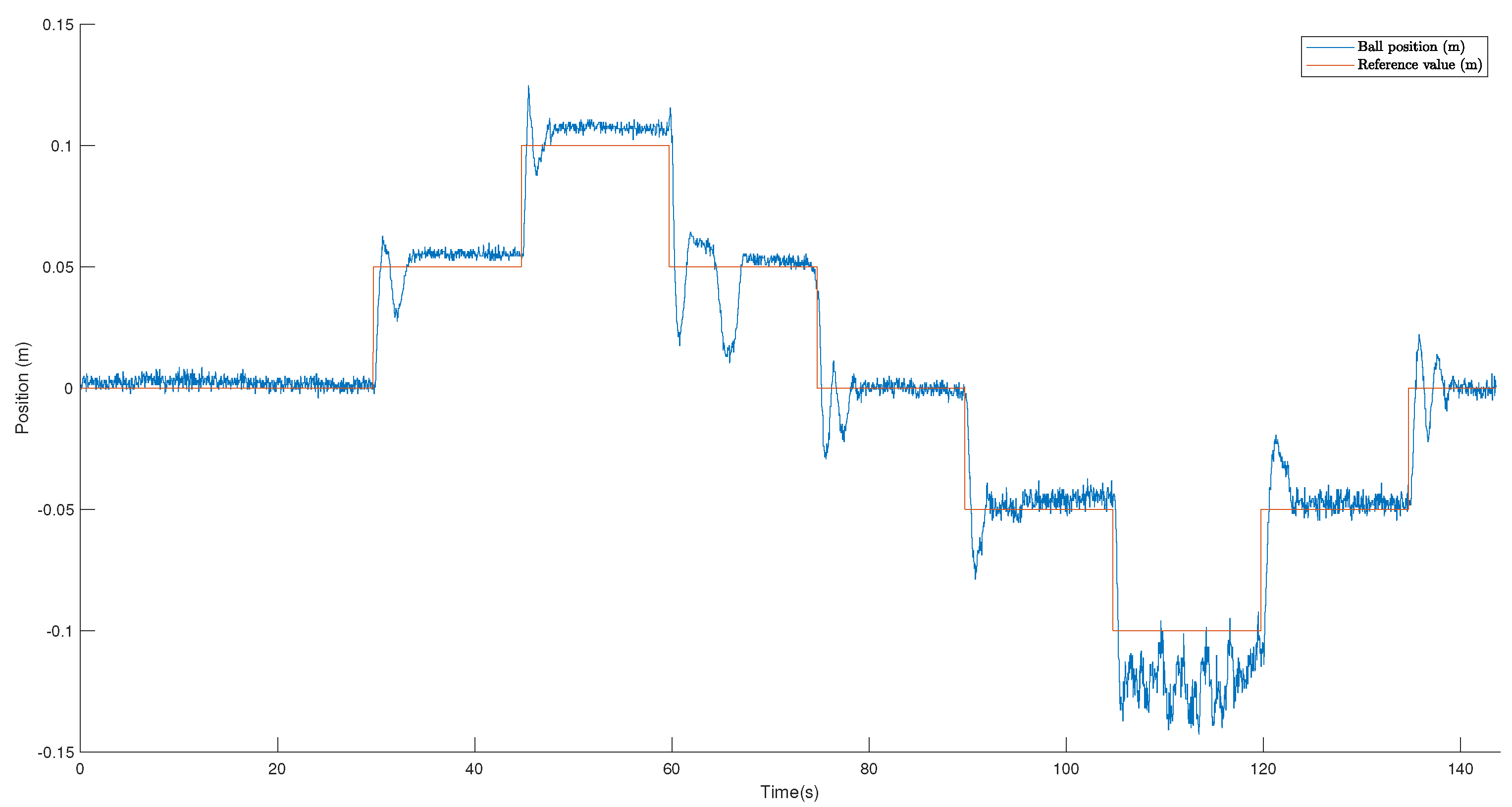
The master controller design requirements are $t_r$ less than 1 s and $M_p$ less than 30%. The controller parameters were obtained using the MATLAB Sisotool tool, resulting in $k_p$ = 0.782 and $k_d$ = 0.34. However, after carrying out the experimentation, manual adjustments were made to improve the control of the ball on the rail, resulting in $k_p=0.935$, $k_d=0.195$, and the addition of $k_i=0.075$. These were in order to eliminate the error in the stationary state caused by the non-linearities of the plant. Figure 21 shows the position of the ball on the rail in contrast to the desired reference value. The overshoot achieved was lower than expected, having a value of 25%. On the other hand, a rise time of 0.77 s was reached.

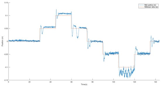
Figure 21. Position of the ball on the rail in contrast to the desired reference value.

It can be seen that the reference value of 0.1 m has the most significant control error. This is because the position is furthest from the sensor, so the measurement error directly affects control. In the same way, there is not a constant steady-state value. On the other hand, there is a slight oscillation in the position. This is due to the resolution of the sensor and its constant oscillation of the distance measurement.

3. Practical Sequence and Project Evaluation

The evaluation was carried out taking into account the ABET criteria, such as [22,37]:

• College-level mathematics: College -level mathematics consist of mathematics that require a degree of mathematical sophistication. Some examples of college-level math include calculus, differential equations, probability, statistics, linear algebra, and discrete math.
• Complex Engineering Problems: Complex engineering problems include one or more of the following characteristics: they involve far-reaching or conflicting technical problems that have no obvious solution; address problems not covered by current standards and codes; involve diverse groups of stakeholders, including many components or sub-issues, involving multiple disciplines or having significant consequences in various contexts.
• Engineering Design: This is creating a system, component, or process to meet desired needs and specifications within constraints. It is an iterative, creative, and decision-making process in which basic science, mathematics, and engineering science are applied to turn resources into solutions.
• Engineering sciences: These build on basic math and science, but take knowledge further into the creative application needed to solve engineering problems. These studies bridge basic mathematics and science on the one hand and engineering practice on the other.
• Teamwork: A team involves more than one person working toward a common goal and should include people from diverse backgrounds, skills, or perspectives.

The following aspects in students are sought to be developed:

• The ability to identify, formulate, and solve complex engineering problems by applying engineering, science, and mathematics principles.
• The ability to apply engineering design to produce solutions that meet specific needs considering public health, safety, and welfare, as well as global, cultural, social, environmental, and economic factors.
• Functioning effectively on a team whose members provide leadership, create a collaborative and inclusive environment, set goals, plan tasks, and meet objectives.
• The ability to develop and perform appropriate experimentation, analyze and interpret data, and use engineering judgment to conclusions.
• The ability to acquire and apply new knowledge as needed using appropriate learning strategies.

The practices necessary to carry out the methodology described above and reinforce the objectives mentioned at the beginning of this section are described below in Table 6.

Table 6. Description of the practices that must be carried out for the completion of the project.

Practice	Objective	Duration	Expected Results
1. Hardware description: In this practice, the electronics and hardware are designed and implemented to carry out the ball and beam.	In this practice, the electronics and hardware are designed and implemented to carry out the ball and beam.	15 h	It is expected that the plant (ball and beam) is in operation, which involves a printed circuit board, the rail, stop pieces, and sensor support.
2. Graphical user interface: In this practice, the operation of the interface designed for this work is understood, and, in turn, the student is given the necessary tools to develop their own.	The mathematics behind motor model identification is understood. This knowledge is used to develop a user interface focused on DC motor identification based on the interface presented.	10 h	A user interface is expected to be capable of calculating the constants of the motor transfer function and the poles required to achieve the control instruction.
3. Identification of DC motor parameters: The motor function was calculated with the interface developed in the previous practice.	That the student can read the data of the encoder to obtain the necessary data for the calculation of the transfer function of the motor. For this objective, it is essential to develop and strengthen knowledge of programming and communication protocols in specific UART.	10 h	It is expected to have the transfer function that describes the motor and the necessary code for implementing a PID controller.
4. Design and implementation of a PD position controller: Using the locus of the roots, calculate the PID control constants and implement it with the code developed for motor position control in the previous practice.	To understand the importance and effect of each PID constant, in addition to understanding and carrying out the design and implementation of the motor shaft position control, and in addition to facing the non-linearities that real systems present.	20 h	Position control of the motor shaft that complies with the defined instructions $Mp\le 30\%$ and $t_r\le 0.1$ s.
5. Calibration of the distance sensor and identification of the parameters of the ball on the rail: Once the position control of the motor is obtained, the position sensor is calibrated, taking the center as 0. In addition, the function that models the fall of the ball on the rail is calculated.	In this practice, the objective is to implement the distance sensor, which involves its programming and understanding of the I2C communication protocol, in addition to calculating the c of the transfer function that represents the fall of the ball in order to close the control diagram in the next step.	5 h	It is expected to have the reading of the position of the ball on the rail in a range of [−0.15 m 0.15 m] in conjunction with the position control of the motor.
6. Design and implementation of a PID distance controller: The PID controller of the master control loop is calculated. Finally, the entire project for controlling the ball on the rail is implemented.	To complete the control loops and carry out the reduction for the calculation of the master PID control. In turn, to develop the software to control the position of the ball on the rail. Finally, to implement it and adjust the calculated control due to non-linearities that were not foreseen in the modeling of the plant.	25 h	It is expected that, at the end of this practice, the entire plant is operational for the final delivery of the project.

Finally, a proposal for an evaluation rubric based on the ABET requirements is presented, which is presented in Table 7. The teacher must assign a note in one of the intervals in which each one of the described criteria was met. In addition, the quality in the development of each one of the points must be considered.

Table 7. The rubric used for evaluating the specific indicators based on ABET.

Specific Indicators	Criteria	Grade
		90–100	70–89	60–69	0–59
The ability to apply the knowledge, techniques, skills, and modern tools that will be applied in engineering and technology activities. The student works in teams	(1) LabVIEW programming (2) Knowledge about digital systems (3) Ability to make measurements with sensors (4) Performs signal conditioning of sensors (5) PCB fabrication according to specific standards (6) Use of communication interfaces (7) Contribute to the team with their theoretical knowledge	Criteria 1 to 6 were almost completed	Criteria 1 to 5 were completed	Criteria 1 to 4 were completed	Criteria 1 to 2 were almost completed
The ability to apply knowledge of mathematics, science, engineering, and technology to technological problems that require an application of principles and extensive practical skills	(1) Design and implementation of the controller (2) Application of techniques for tuning the controller (3) Application of mathematical method for identification of parameters of the DC motor (4) Use of auxiliary software for controller design	Criteria 1 to 4 were completed	Criteria 1 to 3 were completed	Criteria 1 to 2 were completed	Criteria 1 was completed
The ability to perform tests, standard measurements, and analyze and interpret the experiments	(1) Correct use of units of measurement and scaling (2) Correct use of the sensors (3) Correct interpretation of the output graphs (4) Interpretation of information on applied techniques (root locus)	Criteria 1 to 4 were completed	Criteria 1 to 3 were completed	Criteria 1 to 2 were completed	Criterion 1 was completed
The student synthesizes codes with specialized software	(1) Microcontrollers programming (2) Knowledge to design mechanical implementation (3) Implementation of communication protocols (4) Perform a debugging, verification, and optimization of codes using simulation	Criteria 1 to 4 were completed	Criteria 1 to 3 were completed	Criteria 1 to 2 were completed	Criterion 1 was completed
The ability to write technical reports and express their ideas, as well as the ability to identify and use technical documentation	(1) Write the laboratory report in detail and in a structured, detailed manner (2) Explain the results and conclusions in detail (3) Include the figures and equations necessary for an appropriate explanation (4) Correctly cites the bibliographical sources (5) Write with appropriate language and correct grammar and spelling	Criteria 1 to 5 were completed	Criteria 1 to 4 were completed	Criteria 1 to 3 were completed	Criteria 1 to 2 were completed

4. Discussion

This project is ideal for engineering education and is based on the objectives of the Accreditation Board for Engineering and Technology (ABET).

The ball and beam project allows students to explore different types of control, such as PID control, LQR control, model predictive control (MPC) control, etc. Students can experiment with different configurations and evaluate their performance by measuring parameters such as the rise time, settling time, and desired position-holding accuracy.

Furthermore, this project allows students to learn about model identification and parameter estimation, which is essential for designing automatic control systems. It also allows them to apply theoretical concepts to a physical system and see how they work in practice. Another important aspect is that this project is scalable and can be used to teach students about different levels of complexity in control systems. For example, the students can start with a simple control system and increase the complexity as they gain more experience and skills.

In addition to its teaching application, the ball and beam project provides guidelines for developing skills for practical applications in industry. For example, it can be used to control the position of objects in manufacturing processes, such as the position of parts on a production line. It can also be used in the aerospace industry to control the position of components in flight.

In addition, the detailed example of system development and application also provides students with meaningful hands-on experience in which they can apply and understand the concepts and theories that they are learning.

5. Conclusions

Some of the essential aspects in this work are the various problems that are presented to the students inherent to the hardware development and implementation process, such as a backlash effect in the motor, which causes the rod to lean towards one of the sides, which does not allow the ball to be correctly centered and makes it difficult to tune the control. Another negative aspect that the student should take into account is dry friction. This causes a higher voltage when moving the motor shaft correctly. In most cases, the hardware difficulties drive the simulation aspects to be inconsistent with reality since ideal instruments and materials are considered to formulate mathematical models. It should be noted that care must be taken with the design of the hardware developed in the methodology of this work since, if performed incorrectly, it would be impossible to identify the plant correctly. It is important to highlight that, on many occasions, the student finds that even though the hardware is in the best possible state, the non-linearities caused by the prototype are not capable of exceeding the design requirements, so they must choose to try to compensate for this through the use of software or by making changes to the components used. Another problem that students may need help with is the correct selection of the sample time since, with a meager time, the system cannot be controlled. On the other hand, a very high sample time generates communication errors. It must be considered that the inner loop must be faster than the outer loop. The proposed platform, methodology, and evaluation were designed to support and complement the engineering education process. It is a free access tool that can be included in the student’s training and developed from home. This platform covers various important areas in engineering, such as electronics, project design, instrumentation, control, and programming. Finally, the platform has the versatility to be controlled by various methodologies, such as fuzzy control, intelligent control, etc. Moreover, this project fits outcomes of ABET, allowing the students to fulfill the skills required globally.

References

- Rodriguez-Segura, L.; Zamora-Antuñano, M.A.; Rodriguez-Resendiz, J.; Paredes-García, W.J.; Altamirano-Corro, J.A.; Cruz-Pérez, M.Á. Teaching Challenges in COVID-19 Scenery: Teams Platform-Based Student Satisfaction Approach. Sustainability 2020, 12, 7514. [Google Scholar] [CrossRef]
- Wang, C.; Song, W.; Hu, X.; Yan, S.; Zhang, X.; Wang, X.; Chen, W. Depressive, anxiety, and insomnia symptoms between population in quarantine and general population during the COVID-19 pandemic: A case-controlled study. BMC Psychiatry 2021, 21, 1–9. [Google Scholar] [CrossRef]
- La Comisión Económica para América Latina y el Caribe (CEPAL). La Educación en Tiempos de la Pandemia de COVID-19; UNESCO: Paris, France, 2020. [Google Scholar]
- Goodwin, G.C.; Medioli, A.M.; Sher, W.; Vlacic, L.B.; Welsh, J.S. Emulation-based virtual laboratories: A low-cost alternative to physical experiments in control engineering education. IEEE Trans. Educ. 2011, 54, 48–55. [Google Scholar] [CrossRef]
- Bernstein, D.S. Control experiments and what I learned from them: A personal journey. IEEE Control Syst. 1998, 18, 81–88. [Google Scholar]
- Yao, S.; Liu, X.; Zhang, Y.; Cui, Z. Research on solving nonlinear problem of ball and beam system by introducing detail-reward function. Symmetry 2022, 14, 1883. [Google Scholar] [CrossRef]
- Uyanik, I.; Catalbas, B. A low-cost feedback control systems laboratory setup via Arduino-Simulink interface. Comput. Appl. Eng. Educ. 2018, 26, 718–726. [Google Scholar] [CrossRef]
- Martínez-Prado, M.A.; Rodríguez-Reséndiz, J.; Gómez-Loenzo, R.A.; Camarillo-Gómez, K.A.; Herrera-Ruiz, G. Short informative title: Towards a new tendency in embedded systems in mechatronics for the engineering curricula. Comput. Appl. Eng. Educ. 2019, 27, 603–614. [Google Scholar] [CrossRef]
- Valero, M. Challenges, difficulties and barriers for engineering higher education. J. Technol. Sci. Educ. 2022, 12, 551. [Google Scholar] [CrossRef]
- Mahmoodabadi, M.J.; Shahangian, M.M. A new multi-objective artificial bee colony algorithm for optimal adaptive robust controller design. IETE J. Res. 2022, 68, 1251–1264. [Google Scholar] [CrossRef]
- Ocampo-López, C.; Castrillón-Hernández, F.; Alzate-Gil, H. Implementation of integrative projects as a contribution to the major design experience in Chemical Engineering. Sustainability 2022, 14, 6230. [Google Scholar] [CrossRef]
- Ker, C.C.; Lin, C.E.; Wang, R.T. A ball and beam tracking and balance control using magnetic suspension actuators. Int. J. Control 2007, 80, 695–705. [Google Scholar] [CrossRef]
- De la Torre, L.; Guinaldo, M.; Heradio, R.; Dormido, S. The Ball and Beam System: A Case Study of Virtual and Remote Lab Enhancement With Moodle. IEEE Trans. Indus. Inf. 2015, 11, 934–945. [Google Scholar] [CrossRef]
- Candelas, F.A.; García, G.J.; Puente, S.; Pomares, J.; Jara, C.A.; Pérez, J.; Mira, D.; Torres, F. Experiences on using Arduino for laboratory experiments of Automatic Control and Robotics. IFAC-PapersOnLine 2015, 48, 105–110. [Google Scholar] [CrossRef]
- González-Vargas, A.M.; Serna-Ramirez, J.M.; Fory-Aguirre, C.; Ojeda-Misses, A.; Cardona-Ordoñez, J.M.; Tombé-Andrade, J.; Soria-López, A. A low-cost, free-software platform with hard real-time performance for control engineering education. Comput. Appl. Eng. Educ. 2019, 27, 406–418. [Google Scholar] [CrossRef]
- Muftah, M.N.; Faudzi, A.A.M.; Sahlan, S.; Mohamaddan, S. Intelligent position control for intelligent pneumatic actuator with ball-beam (IPABB) system. Appl. Sci. 2022, 12, 11089. [Google Scholar] [CrossRef]
- Rahmat, M.F.; Wahid, H.; Wahab, N.A. Application of intelligent controller in a ball and beam control system. Int. J. Smart Sens. Intell. Syst. 2010, 3, 45–60. [Google Scholar] [CrossRef]
- Abu Rmilah, M.H.Y.; Hassan, M.A.; Bin Mardi, N.A. A PC-based simulation platform for a quadcopter system with self-tuning fuzzy PID controllers. Comput. Appl. Eng. Educ. 2016, 24, 934–950. [Google Scholar] [CrossRef]
- Cruz-Miguel, E.E.; Rodríguez-Reséndiz, J.; García-Martínez, J.R.; Camarillo-Gómez, K.A.; Pérez-Soto, G.I. Field-programmable gate array-based laboratory oriented to control theory courses. Comput. Appl. Eng. Educ. 2019, 27, 1253–1266. [Google Scholar] [CrossRef]
- Odry, Á.; Fullér, R.; Rudas, I.J.; Odry, P. Fuzzy control of self-balancing robots: A control laboratory project. Comput. Appl. Eng. Educ. 2020, 28, 512–535. [Google Scholar] [CrossRef]
- Jiménez-Ramírez, O.; Cárdenas-Valderrama, J.A.; Ordoñez-Sánchez, A.A.; Quiroz-Juárez, M.A.; Vázquez-Medina, R. Digital proportional-derivative controller implemented in low-resource microcontrollers. Comput. Appl. Eng. Educ. 2020, 28, 1671–1682. [Google Scholar] [CrossRef]
- Gutiérrez, C.A.G.; Reséndiz, J.R.; Santibáñez, J.D.M.; Bobadilla, G.M. A model and simulation of a five-degree-of-freedom robotic arm for mechatronic courses. IEEE Lat. Am. Trans. 2014, 12, 78–86. [Google Scholar] [CrossRef]
- Garduno-Aparicio, M.; Rodriguez-Resendiz, J.; Macias-Bobadilla, G.; Thenozhi, S. A multidisciplinary industrial robot approach for teaching mechatronics-related courses. IEEE Trans. Educ. 2018, 61, 55–62. [Google Scholar] [CrossRef]
- Dizon, J.R.C.; Gache, C.C.L.; Cascolan, H.M.S.; Cancino, L.T.; Advincula, R.C. Post-processing of 3D-printed polymers. Technologies 2021, 9, 61. [Google Scholar] [CrossRef]
- Yang, J.; Wu, H.; Hu, L.; Li, S. Robust predictive speed regulation of converter-driven DC motors via a discrete-time reduced-order GPIO. IEEE Trans. Ind. Electron. 2019, 66, 7893–7903. [Google Scholar] [CrossRef]
- Nise, N. Control Systems Engineering, 6th ed.; John Wiley & Sons, Inc.: Hoboken, NJ, USA, 2011. [Google Scholar]
- Dorf, R.; Bishop, R. Modern Control Systems, 13th ed.; Pearson, Upper Saddle River, NJ, USA, 2016, 13th ed.Pearson: Upper Saddle River, NJ, USA.
- Aguado-Behar, A.; Martínez-Iranzo, M. Identificación y Control Adaptativo, 1st ed.; Prentice-Hall: Madrid, Spain, 2003; p. 280. [Google Scholar]
- Angeles, J. Fundamentals of Robotic Mechanical Systems, 3rd ed.; Springer: New York, NY, USA, 2007; p. 549. [Google Scholar]
- Hernández-Guzmán, V.M.; Silva-Ortigoza, R.; Carrillo-Serrano, R.V. Control Automático: Teoría de Diseño, Construcción de Prototipos, Modelado, Identificación y Pruebas Experimentales, 1st ed.; Colección CIDETEC del Instituto Politécnico Nacional: Distrito Federal, México, 2013. [Google Scholar]
- Mehedi, I.M.; Jeza Aljohani, A.; Mottahir Alam, M.; Mahmoud, M.; Abdulaal, M.J.; Bilal, M.; Alasmary, W. Intelligent dynamic inversion controller design for ball and beam system. Comput. Mater. Contin. 2022, 72, 2341–2355. [Google Scholar] [CrossRef]
- Srivastava, V.; Srivastava, S. Hybrid optimization based PID control of ball and beam system. J. Intell. Fuzzy Syst. 2022, 42, 919–928. [Google Scholar] [CrossRef]
- Peters, A.; Vargas, F.; Garrido, C.; Andrade, C.; Villenas, F. Pl-toon: A low-cost experimental platform for teaching and research on decentralized cooperative control. Sensors 2021, 21, 2072. [Google Scholar] [CrossRef]
- Ogata, K. Ingeniería de Control Moderna; Pearson Educación: London, UK, 2010. [Google Scholar]
- Tang, W.J.; Liu, Z.T.; Wang, Q. DC motor speed control based on system identification and PID auto tuning. In Proceedings of the 2017 36th Chinese Control Conference (CCC), Dalian, China, 26–28 July 2017. [Google Scholar]
- Xie, C.; Zhao, X.; Li, K.; Zou, J.; Guerrero, J.M. A new tuning method of multiresonant current controllers for grid-connected voltage source converters. IEEE J. Emerg. Sel. Top. Power Electron. 2019, 7, 458–466. [Google Scholar] [CrossRef]
- Torres-Salinas, H.; Rodríguez-Reséndiz, J.; Estévez-Bén, A.A.; Cruz Pérez, M.A.; Sevilla-Camacho, P.Y.; Perez-Soto, G.I. A Hands-On Laboratory for Intelligent Control Courses. Appl. Sci. 2020, 10, 9070. [Google Scholar] [CrossRef]
Disclaimer/Publisher’s Note: The statements, opinions and data contained in all publications are solely those of the individual author(s) and contributor(s) and not of MDPI and/or the editor(s). MDPI and/or the editor(s) disclaim responsibility for any injury to people or property resulting from any ideas, methods, instructions or products referred to in the content. |
© 2023 by the authors. Licensee MDPI, Basel, Switzerland. This article is an open access article distributed under the terms and conditions of the Creative Commons Attribution (CC BY) license (https://creativecommons.org/licenses/by/4.0/).