
Multimodal Semantic Segmentation in Autonomous Driving: A Review of Current Approaches and Future Perspectives


Abstract
:1. Introduction
1.1. Semantic Segmentation with Deep Learning
1.2. Outline
2. Multimodal Data Acquisition and Preprocessing
2.1. RGB Cameras
2.2. Thermal Cameras
2.3. Depth Cameras
- the resilience to environmental conditions;
- the working range;
- the sparsity of the output depthmap; and
- the cost.
2.3.1. Stereo Camera
2.3.2. Time-of-Flight
2.3.3. LiDAR
- spherical projection;
- perspective projection; and
- bird’s-eye view.
2.3.4. RADAR
2.4. Position and Navigation Systems
3. Datasets
- modalities provided (i.e., type of available sensors);
- tasks supported (i.e., provided labeling information);
- data variability offered (i.e., daytime, weather, season, location, etc.); and
- acquisition domain (i.e., real or synthetic).
Summary
- KITTI
- [8,65,66,67] was the first large-scale dataset to tackle the important issue of multimodal data in autonomous vehicles. The KITTI vision benchmark was introduced in 2012 and contains a real-world 6-h-long sequence recorded using a LiDAR, an IMU, and two stereo setups (with one grayscale and one color camera each). Although the complete suite is very extensive (especially for depth estimation and object detection), the authors did not focus much on the semantic labeling process, opting to label only 200 training samples for semantic (and instance) segmentation and for optical flow.
- Cityscapes
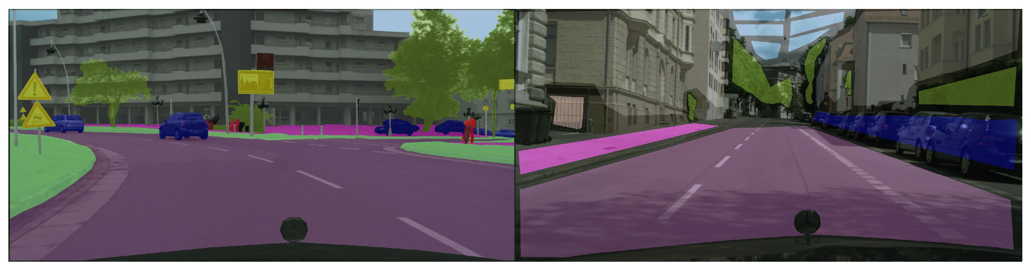
- [68] became one of the most common semantic segmentation datasets for autonomous driving benchmarks. It is a real-world dataset containing 5000 finely labeled, high-definition (2048 × 1024) images captured in multiple German cities. Additionally, the authors provide 25,000 coarsely labeled samples—polygons rather than object borders, with many unlabeled areas (see Figure 3)—to improve deep architectures’ performance through data variability. The data was captured with a calibrated and rectified stereo setup in high-visibility conditions, allowing the authors to provide high-quality estimated depthmaps for each of the 30,000 samples. Given its popularity in semantic segmentation settings, this dataset is also one of the most used for monocular depth estimation or 2.5D segmentation tasks.
- Lost and Found
- [69] is an interesting road-scene dataset that tackles lost cargo scenarios, it includes pixel-level segmentation of the road and of the extraneous objects present on the surface. It was introduced in 2016 and includes around 2000 samples. The dataset comprises 112 stereo video sequences with 2104 annotated frames in a real-world scenario.
- Synthia
- [70,71,72] is one of the oldest multimodal synthetic datasets providing labeled semantic segmentation samples. First introduced in 2016, it provides color, depth, and semantic information generated from the homonym simulator. The authors tackled data diversity by simulating the four seasons, by rendering the dataset samples from multiple PoVs, not only from road-view, but also from building height, and by considering day/night times. The dataset provides multiple versions, but only one supports (partially) the Cityscapes dataset label-set; it contains 9400 total samples.
- Virtual KITTI
- [73,74] is an extension of the KITTI dataset. It is a synthetic dataset produced in Unity (https://unity.com/ (accessed on 21 July 2022) ) which contains scenes modeled after the ones present in the original KITTI dataset. The synthetic nature of the dataset allowed the authors to produce a much greater number of labeled samples than those present in KITTI, while also maintaining a higher precision (due to the automatic labeling process). Unfortunately, the dataset does not provide labels for the LiDAR pointclouds.
- MSSSD/MF
- [75] is a real-world dataset and one of the few that provides multispectral (thermal + color) information. It is of relatively small size, with only 1.5k samples, recorded in day and night scenes. Regardless, it represents an important benchmark for real-world applications, because thermal cameras are one of the few dense sensors resilient to low-visibility conditions such as fog or rain for which consumer-grade options exist.
- RoadScene-Seg
- [76] is real-world dataset that provides 200 unlabeled road-scene images captured with an aligned color + infrared setup. Given the absence of labels, the only validation metric supported for architectures in this dataset is a qualitative evaluation by humans.
- AtUlm
- [77] is a non-publicly available real-world dataset developed by Ulm University in 2019. It has been acquired with a grayscale camera and 4 LiDARs. In total the dataset contains 1446 finely annotated samples (grayscale images).
- nuScenes
- [78] is a real-world dataset and one of the very few providing RADAR information. It is the standard for architectures aiming to use such sensor modality. The number of sensors provided is very impressive, as the dataset contains samples recorded from six top ring-cameras (two of which form a stereo setup), one top-central LiDAR, five ring RADARs placed at headlight level, and an IMU. The labeled samples are keyframes extracted with a frequency of 2 Hz from the recorded sequences, totaling 40k samples. The environmental variability lies in the recording location. The cities of Boston and Singapore were chosen as they offer different traffic handedness (Boston right-handed, Singapore left-handed).
- Semantic KITTI
- [35] is an extension to the KITTI dataset. Here the authors took on the challenge of labeling in a point-wise manner all the LiDAR sequences recorded in the original set. It has rapidly become one of the most common benchmarks for LiDAR semantic segmentation, especially thanks to the significant number of samples made available.
- ZJU
- [79] is a real-world dataset and the only among the one listed supporting the light polarization modality. It was introduced in 2019 and features 3400 labeled samples provided with color, (stereo) depth, light polarization, and an additional fish-eye camera view to cover the whole scene.
- A2D2
- [80] is another real-world dataset which focuses highly on the multimodal aspect of the data provided. It was recorded by a research team from the AUDI car manufacturer and provides five ring LiDARs, six ring cameras (two of which form a stereo setup) and an IMU. The semantic segmentation labels refer to both 2D images and LiDAR pointclouds, for a total of 41k samples. The daytime variability is very limited, offering only high-visibility day samples. The weather variability is slightly better, as it was changing throughout the recorded sequences, but no control over the conditions is offered.
- ApolloScape
- [81] is a large-scale real-world dataset that supports a multitude of different tasks (semantic segmentation, lane segmentation, trajectory estimation, depth estimation, and more). As usual, we focus on the semantic segmentation task, for which ApolloScape provides ∼150k labeled RGB images. Together with the color samples, the dataset also provides depth information. Unfortunately the depth maps contain only static objects, and all information about vehicles or other road occupants is missing. This precludes the possibility of directly exploiting the dataset in multimodal settings because a deployed agent wouldn’t have access to such static maps.
- DDAD
- [82] is a real-world dataset developed by the Toyota Research Institute, whose main focus is on monocular depth estimation. The sensors provided include six ring cameras and four ring LiDARs. The data was recorded in seven cities across two states: San Francisco, the Bay Area, Cambridge, Detroit, and Ann Arbor in the USA, and Tokyo and Odaiba in Japan. The dataset provides semantic segmentation labels only for the validation and test (non-public) sets, significantly restricting its use-case.
- KITTI 360
- [83] is a real-world dataset first released in 2020, which provides many different modalities (Stereo Color, LiDAR, Spherical, and IMU) and labeled segmentation samples for them. The labeling is performed in the 3D space, and the 2D labels are extracted by re-projection. In total, the dataset contains 78K labeled samples. Like KITTI, the dataset is organized in temporal sequences, recorded from a synchronized sensor setup mounted on a vehicle. As such, it offers very limited environmental variability.
- WoodScape
- [84] is another real-world dataset providing color and LiDAR information. As opposed to its competitors, its 2D information is extracted only by using fish-eye cameras. In particular, the dataset provides information coming from four fish-eye ring cameras and a single top-LiDAR (360° coverage), recorded from more than ten cities in five different states. In total, the dataset contains 10k 2D semantic segmentation samples.
- EventScape
- SELMA
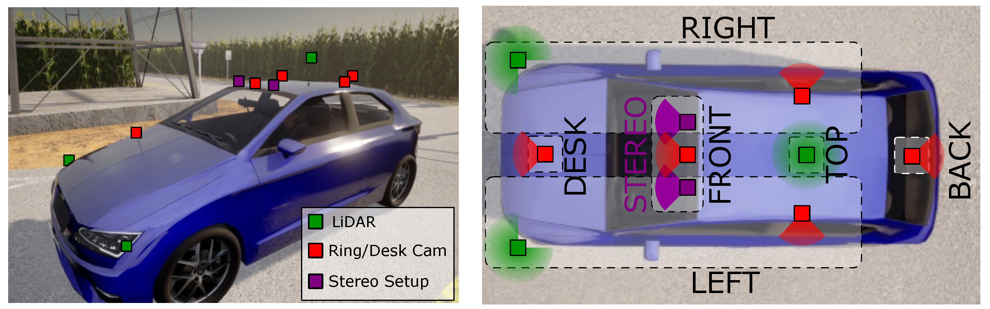
- [39] is a very recent (2022) synthetic dataset developed in a modified CARLA simulator [96] whose goal is to provide multimodal data in a multitude of environmental conditions, while also allowing a researcher to control such conditions. It is heavily focused on semantic segmentation, providing labels for all of the sensors offered (seven co-placed RGB/depth cameras, and three LiDARs). The environmental variability takes the form of three daytimes (day, sunset, night), nine weather conditions (clear, cloudy, wet road, wet road and cloudy, soft/mid-level/heavy rain, mid-level/heavy fog), and 8 synthetic towns. The dataset contains 31k unique scenes recorded in all 27 environmental conditions, resulting in 800k samples for each sensor.
4. Multimodal Segmentation Techniques in Autonomous Driving
- modalities used for the fusion;
- datasets used for training and validation;
- approach to feature fusion (e.g., sum, concatenation, attention, etc.); and
- fusion network location (e.g., encoder, decoder, specific modality branch, etc.).
4.1. Semantic Segmentation from RGB and Depth Data
4.2. Semantic Segmentation from RGB and LiDAR Data
4.3. Pointcloud Semantic Segmentation from RGB and LiDAR Data
4.4. Semantic Segmentation from Other Modalities
5. Conclusions and Outlooks
Author Contributions
Funding
Institutional Review Board Statement
Informed Consent Statement
Data Availability Statement
Conflicts of Interest
Abbreviations
| A2D2 | Audi Autonomous Driving Dataset. |
| CV | Computer Vision. |
| DARPA | Defense Advanced Research Projects Agency. |
| DDAD | Dense Depth for Autonomous Driving. |
| dToF | Direct Time-of-Flight. |
| FCN | Fully Convolutional Network. |
| FoV | Field-of-View. |
| FPN | Feature Pyramid Network. |
| GNSS | Global Navigation Satellite Systems. |
| GPS | Global Positioning System. |
| IMU | Inertial Measurement Unit. |
| iToF | Indirect Time-of-Flight. |
| LiDAR | Light Detection and Ranging. |
| mIoU | mean Intersection over Union. |
| MLP | Multi-Layer Perceptron. |
| MSSSD | Multi-Spectral Semantic Segmentation Dataset. |
| MVSEC | MultiVehicle Stereo Event Camera. |
| NLP | Natural Language Processing. |
| PoV | Point of View. |
| RADAR | Radio Detection and Ranging. |
| SELMA | SEmantic Large-scale Multimodal Acquisitions. |
| SGM | Semi-Global Matching. |
| SRM | Snow Removal Machine. |
| SS | Semantic Segmentation. |
| SSMA | Self-Supervised Model Adaptation. |
| SSW | Snowy SideWalk. |
| ToF | Time-of-Flight. |
| VGG | Visual Geometry Group. |
| ViT | Vision Tranformers. |
References
- Yurtsever, E.; Lambert, J.; Carballo, A.; Takeda, K. A survey of autonomous driving: Common practices and emerging technologies. IEEE Access 2020, 8, 58443–58469. [Google Scholar] [CrossRef]
- Liu, L.; Lu, S.; Zhong, R.; Wu, B.; Yao, Y.; Zhang, Q.; Shi, W. Computing Systems for Autonomous Driving: State of the Art and Challenges. IEEE Internet Things J. 2021, 8, 6469–6486. [Google Scholar] [CrossRef]
- Wang, J.; Liu, J.; Kato, N. Networking and Communications in Autonomous Driving: A Survey. IEEE Commun. Surv. Tutor. 2019, 21, 1243–1274. [Google Scholar] [CrossRef]
- Broggi, A.; Buzzoni, M.; Debattisti, S.; Grisleri, P.; Laghi, M.C.; Medici, P.; Versari, P. Extensive Tests of Autonomous Driving Technologies. IEEE Trans. Intell. Transp. Syst. 2013, 14, 1403–1415. [Google Scholar] [CrossRef]
- Okuda, R.; Kajiwara, Y.; Terashima, K. A survey of technical trend of ADAS and autonomous driving. In Proceedings of the Technical Papers of 2014 International Symposium on VLSI Design, Automation and Test, Hsinchu, Taiwan, 28–30 April 2014; pp. 1–4. [Google Scholar] [CrossRef]
- Bremond, F. Scene Understanding: Perception, Multi-Sensor Fusion, Spatio-Temporal Reasoning and Activity Recognition. Ph.D. Thesis, Université Nice Sophia Antipolis, Nice, France, 2007. [Google Scholar]
- Gu, Y.; Wang, Y.; Li, Y. A survey on deep learning-driven remote sensing image scene understanding: Scene classification, scene retrieval and scene-guided object detection. Appl. Sci. 2019, 9, 2110. [Google Scholar] [CrossRef] [Green Version]
- Geiger, A.; Lenz, P.; Urtasun, R. Are we ready for Autonomous Driving? The KITTI Vision Benchmark Suite. In Proceedings of the Conference on Computer Vision and Pattern Recognition (CVPR), Providence, RI, USA, 16–21 June 2012. [Google Scholar]
- Fan, R.; Wang, L.; Bocus, M.J.; Pitas, I. Computer stereo vision for autonomous driving. arXiv 2020, arXiv:2012.03194. [Google Scholar]
- Zanuttigh, P.; Marin, G.; Dal Mutto, C.; Dominio, F.; Minto, L.; Cortelazzo, G.M. Time-of-Flight and Structured Light Depth Cameras; Springer International Publishing: Cham, Switzerland, 2016. [Google Scholar]
- Brostow, G.J.; Shotton, J.; Fauqueur, J.; Cipolla, R. Segmentation and recognition using structure from motion point clouds. In Proceedings of the European Conference on Computer Vision, Marseille, France, 12–18 October 2008; pp. 44–57. [Google Scholar]
- Sturgess, P.; Alahari, K.; Ladicky, L.; Torr, P.H. Combining appearance and structure from motion features for road scene understanding. In Proceedings of the BMVC-British Machine Vision Conference, London, UK, 7–10 September 2009. [Google Scholar]
- Zhang, C.; Wang, L.; Yang, R. Semantic segmentation of urban scenes using dense depth maps. In Proceedings of the European Conference on Computer Vision, Heraklion, Greece, 5–11 September 2010; pp. 708–721. [Google Scholar]
- Long, J.; Shelhamer, E.; Darrell, T. Fully convolutional networks for semantic segmentation. In Proceedings of the IEEE Conference on Computer Vision and Pattern Recognition, Boston, MA, USA, 7–12 June 2015; pp. 3431–3440. [Google Scholar]
- Simonyan, K.; Zisserman, A. Very deep convolutional networks for large-scale image recognition. arXiv 2014, arXiv:1409.1556. [Google Scholar]
- He, K.; Zhang, X.; Ren, S.; Sun, J. Deep residual learning for image recognition. In Proceedings of the IEEE Conference on Computer Vision and Pattern Recognition, Honolulu, HI, USA, 21–26 July 2016; pp. 770–778. [Google Scholar]
- Howard, A.G.; Zhu, M.; Chen, B.; Kalenichenko, D.; Wang, W.; Weyand, T.; Andreetto, M.; Adam, H. Mobilenets: Efficient convolutional neural networks for mobile vision applications. arXiv 2017, arXiv:1704.04861. [Google Scholar]
- Liu, W.; Rabinovich, A.; Berg, A.C. Parsenet: Looking wider to see better. arXiv 2015, arXiv:1506.04579. [Google Scholar]
- Noh, H.; Hong, S.; Han, B. Learning deconvolution network for semantic segmentation. In Proceedings of the IEEE International Conference on Computer Vision, Santiago, Chile, 11–18 December 2015; pp. 1520–1528. [Google Scholar]
- Lin, T.Y.; Dollár, P.; Girshick, R.; He, K.; Hariharan, B.; Belongie, S. Feature pyramid networks for object detection. In Proceedings of the IEEE Conference on computer Vision and Pattern Recognition, Honolulu, HI, USA, 21–26 July 2017; pp. 2117–2125. [Google Scholar]
- Chen, L.C.; Papandreou, G.; Kokkinos, I.; Murphy, K.; Yuille, A.L. Deeplab: Semantic image segmentation with deep convolutional nets, atrous convolution, and fully connected crfs. IEEE Trans. Pattern Anal. Mach. Intell. 2017, 40, 834–848. [Google Scholar] [CrossRef] [Green Version]
- Chen, L.C.; Zhu, Y.; Papandreou, G.; Schroff, F.; Adam, H. Encoder-decoder with atrous separable convolution for semantic image segmentation. In Proceedings of the European Conference on Computer Vision (ECCV), Munich, Germany, 8–14 September 2018; pp. 801–818. [Google Scholar]
- Vaswani, A.; Shazeer, N.; Parmar, N.; Uszkoreit, J.; Jones, L.; Gomez, A.N.; Kaiser, Ł.; Polosukhin, I. Attention is all you need. In Proceedings of the 31st Conference on Neural Information Processing Systems (NIPS 2017), Long Beach, CA, USA, 4–9 December 2017. [Google Scholar]
- Dosovitskiy, A.; Beyer, L.; Kolesnikov, A.; Weissenborn, D.; Zhai, X.; Unterthiner, T.; Dehghani, M.; Minderer, M.; Heigold, G.; Gelly, S.; et al. An image is worth 16x16 words: Transformers for image recognition at scale. arXiv 2020, arXiv:2010.11929. [Google Scholar]
- Kolesnikov, A.; Dosovitskiy, A.; Weissenborn, D.; Heigold, G.; Uszkoreit, J.; Beyer, L.; Minderer, M.; Dehghani, M.; Houlsby, N.; Gelly, S.; et al. An image is worth 16x16 words: Transformers for image recognition at scale. In Proceedings of the International Conference on Learning Representations (ICLR), Virtual Event, Austria, 3–7 May 2021. [Google Scholar]
- Zheng, S.; Lu, J.; Zhao, H.; Zhu, X.; Luo, Z.; Wang, Y.; Fu, Y.; Feng, J.; Xiang, T.; Torr, P.H.; et al. Rethinking semantic segmentation from a sequence-to-sequence perspective with transformers. In Proceedings of the IEEE/CVF Conference on Computer Vision and Pattern Recognition, Nashville, TN, USA, 20–25 June 2021; pp. 6881–6890. [Google Scholar]
- Xie, E.; Wang, W.; Yu, Z.; Anandkumar, A.; Alvarez, J.M.; Luo, P. SegFormer: Simple and efficient design for semantic segmentation with transformers. Adv. Neural Inf. Process. Syst. 2021, 34, 12077–12090. [Google Scholar]
- Strudel, R.; Garcia, R.; Laptev, I.; Schmid, C. Segmenter: Transformer for semantic segmentation. In Proceedings of the IEEE/CVF International Conference on Computer Vision, Montreal, QC, Canada, 10–17 October 2021; pp. 7262–7272. [Google Scholar]
- Qi, C.R.; Su, H.; Mo, K.; Guibas, L.J. Pointnet: Deep learning on point sets for 3d classification and segmentation. In Proceedings of the IEEE Conference on Computer Vision and Pattern Recognition, Honolulu, HI, USA, 21–26 July 2017; pp. 652–660. [Google Scholar]
- Qi, C.R.; Yi, L.; Su, H.; Guibas, L.J. Pointnet++: Deep hierarchical feature learning on point sets in a metric space. In Proceedings of the 31st Conference on Neural Information Processing Systems (NIPS 2017), Long Beach, CA, USA, 4–9 December 2017. [Google Scholar]
- Hu, Q.; Yang, B.; Xie, L.; Rosa, S.; Guo, Y.; Wang, Z.; Trigoni, N.; Markham, A. Randla-net: Efficient semantic segmentation of large-scale point clouds. In Proceedings of the IEEE/CVF Conference on Computer Vision and Pattern Recognition, Seattle, WA, USA, 13–19 June 2020; pp. 11108–11117. [Google Scholar]
- Tchapmi, L.; Choy, C.; Armeni, I.; Gwak, J.; Savarese, S. SEGCloud: Semantic Segmentation of 3D Point Clouds. In Proceedings of the 2017 International Conference on 3D Vision (3DV), Qingdao, China, 10–12 October 2017; pp. 537–547. [Google Scholar] [CrossRef] [Green Version]
- Wu, B.; Wan, A.; Yue, X.; Keutzer, K. Squeezeseg: Convolutional neural nets with recurrent crf for real-time road-object segmentation from 3d lidar point cloud. In Proceedings of the 2018 IEEE International Conference on Robotics and Automation (ICRA), Brisbane, Australia, 21–25 May 2018; pp. 1887–1893. [Google Scholar]
- Zhu, X.; Zhou, H.; Wang, T.; Hong, F.; Ma, Y.; Li, W.; Li, H.; Lin, D. Cylindrical and asymmetrical 3d convolution networks for lidar segmentation. In Proceedings of the IEEE/CVF Conference on Computer Vision and Pattern Recognition, Nashville, TN, USA, 20–25 June 2021; pp. 9939–9948. [Google Scholar]
- Behley, J.; Garbade, M.; Milioto, A.; Quenzel, J.; Behnke, S.; Stachniss, C.; Gall, J. Semantickitti: A dataset for semantic scene understanding of lidar sequences. In Proceedings of the IEEE/CVF International Conference on Computer Vision, Seoul, Korea, 27 October–2 November 2019; pp. 9297–9307. [Google Scholar]
- Milioto, A.; Vizzo, I.; Behley, J.; Stachniss, C. Rangenet++: Fast and accurate lidar semantic segmentation. In Proceedings of the 2019 IEEE/RSJ International Conference on Intelligent Robots and Systems (IROS), Macao, China, 3–8 November 2019; pp. 4213–4220. [Google Scholar]
- Secci, F.; Ceccarelli, A. On failures of RGB cameras and their effects in autonomous driving applications. In Proceedings of the IEEE 31st International Symposium on Software Reliability Engineering (ISSRE), Coimbra, Portugal, 12–15 October 2020. [Google Scholar]
- Gade, R.; Moeslund, T.B. Thermal cameras and applications: A survey. Mach. Vis. Appl. 2014, 25, 245–262. [Google Scholar] [CrossRef] [Green Version]
- Testolina, P.; Barbato, F.; Michieli, U.; Giordani, M.; Zanuttigh, P.; Zorzi, M. SELMA: SEmantic Large-scale Multimodal Acquisitions in Variable Weather, Daytime and Viewpoints. arXiv 2022, arXiv:2204.09788. [Google Scholar]
- Moreland, K. Why we use bad color maps and what you can do about it. Electron. Imaging 2016, 2016, 1–6. [Google Scholar] [CrossRef] [Green Version]
- Zhou, Y.; Liu, L.; Zhao, H.; López-Benítez, M.; Yu, L.; Yue, Y. Towards Deep Radar Perception for Autonomous Driving: Datasets, Methods, and Challenges. Sensors 2022, 22, 4208. [Google Scholar] [CrossRef]
- Gao, B.; Pan, Y.; Li, C.; Geng, S.; Zhao, H. Are We Hungry for 3D LiDAR Data for Semantic Segmentation? A Survey of Datasets and Methods. IEEE Trans. Intell. Transp. Syst. 2022, 23, 6063–6081. [Google Scholar] [CrossRef]
- Jang, M.; Yoon, H.; Lee, S.; Kang, J.; Lee, S. A Comparison and Evaluation of Stereo Matching on Active Stereo Images. Sensors 2022, 22, 3332. [Google Scholar] [CrossRef]
- Hirschmuller, H. Accurate and efficient stereo processing by semi-global matching and mutual information. In Proceedings of the 2005 IEEE Computer Society Conference on Computer Vision and Pattern Recognition (CVPR’05), San Diego, CA, USA, 20–25 June 2005; Volume 2, pp. 807–814. [Google Scholar]
- Zhou, K.; Meng, X.; Cheng, B. Review of stereo matching algorithms based on deep learning. Comput. Intell. Neurosci. 2020, 2020, 8562323. [Google Scholar] [CrossRef]
- Li, J.; Wang, P.; Xiong, P.; Cai, T.; Yan, Z.; Yang, L.; Liu, J.; Fan, H.; Liu, S. Practical Stereo Matching via Cascaded Recurrent Network with Adaptive Correlation. In Proceedings of the 2022 IEEE Computer Society Conference on Computer Vision and Pattern Recognition (CVPR), New Orleans, LO, USA, 19–24 June 2022. [Google Scholar]
- Tonioni, A.; Tosi, F.; Poggi, M.; Mattoccia, S.; Stefano, L.D. Real-time self-adaptive deep stereo. In Proceedings of the IEEE/CVF Conference on Computer Vision and Pattern Recognition, Long Beach, CA, USA, 15–20 June 2019; pp. 195–204. [Google Scholar]
- Gupta, S.; Girshick, R.; Arbeláez, P.; Malik, J. Learning rich features from RGB-D images for object detection and segmentation. In Proceedings of the European Conference on Computer Vision, Zurich, Switzerland, 6–12 September 2014; pp. 345–360. [Google Scholar]
- Padmanabhan, P.; Zhang, C.; Charbon, E. Modeling and analysis of a direct time-of-flight sensor architecture for LiDAR applications. Sensors 2019, 19, 5464. [Google Scholar] [CrossRef] [Green Version]
- Li, Y.; Ibanez-Guzman, J. Lidar for autonomous driving: The principles, challenges, and trends for automotive lidar and perception systems. IEEE Signal Process. Mag. 2020, 37, 50–61. [Google Scholar] [CrossRef]
- Camuffo, E.; Mari, D.; Milani, S. Recent Advancements in Learning Algorithms for Point Clouds: An Updated Overview. Sensors 2022, 22, 1357. [Google Scholar] [CrossRef] [PubMed]
- Landrieu, L.; Simonovsky, M. Large-scale point cloud semantic segmentation with superpoint graphs. In Proceedings of the IEEE Conference on Computer Vision and Pattern Recognition, Salt Lake City, UT, USA, 18–23 June 2018; pp. 4558–4567. [Google Scholar]
- Wang, Y.; Sun, Y.; Liu, Z.; Sarma, S.E.; Bronstein, M.M.; Solomon, J.M. Dynamic graph cnn for learning on point clouds. ACM Trans. Graph. (TOG) 2019, 38, 1–12. [Google Scholar] [CrossRef] [Green Version]
- Su, H.; Jampani, V.; Sun, D.; Maji, S.; Kalogerakis, E.; Yang, M.H.; Kautz, J. Splatnet: Sparse lattice networks for point cloud processing. In Proceedings of the IEEE Conference on Computer Vision and Pattern Recognition, Salt Lake City, UT, USA, 18–23 June 2018; pp. 2530–2539. [Google Scholar]
- Rosu, R.A.; Schütt, P.; Quenzel, J.; Behnke, S. Latticenet: Fast point cloud segmentation using permutohedral lattices. arXiv 2019, arXiv:1912.05905. [Google Scholar]
- Prophet, R.; Deligiannis, A.; Fuentes-Michel, J.C.; Weber, I.; Vossiek, M. Semantic segmentation on 3D occupancy grids for automotive radar. IEEE Access 2020, 8, 197917–197930. [Google Scholar] [CrossRef]
- Ouaknine, A.; Newson, A.; Pérez, P.; Tupin, F.; Rebut, J. Multi-view radar semantic segmentation. In Proceedings of the IEEE/CVF International Conference on Computer Vision, Montreal, QC, Canada, 10–17 October 2021; pp. 15671–15680. [Google Scholar]
- Kaul, P.; De Martini, D.; Gadd, M.; Newman, P. RSS-Net: Weakly-supervised multi-class semantic segmentation with FMCW radar. In Proceedings of the 2020 IEEE Intelligent Vehicles Symposium (IV), Las Vegas, NV, USA, 19 October–13 November 2020; pp. 431–436. [Google Scholar]
- Bengler, K.; Dietmayer, K.; Farber, B.; Maurer, M.; Stiller, C.; Winner, H. Three decades of driver assistance systems: Review and future perspectives. IEEE Intell. Transp. Syst. Mag. 2014, 6, 6–22. [Google Scholar] [CrossRef]
- Zhou, Y.; Takeda, Y.; Tomizuka, M.; Zhan, W. Automatic Construction of Lane-level HD Maps for Urban Scenes. In Proceedings of the 2021 IEEE/RSJ International Conference on Intelligent Robots and Systems (IROS), Prague, Czech Republic, 27 September–1 October 2021; pp. 6649–6656. [Google Scholar] [CrossRef]
- Guo, C.; Lin, M.; Guo, H.; Liang, P.; Cheng, E. Coarse-to-fine Semantic Localization with HD Map for Autonomous Driving in Structural Scenes. In Proceedings of the 2021 IEEE/RSJ International Conference on Intelligent Robots and Systems (IROS), Prague, Czech Republic, 27 September–1 October 2021; pp. 1146–1153. [Google Scholar] [CrossRef]
- Aggarwal, C.C. Neural Networks and Deep Learning; Springer: Berlin/Heidelberg, Germany, 2018; Volume 10, p. 978. [Google Scholar]
- Yin, H.; Berger, C. When to use what data set for your self-driving car algorithm: An overview of publicly available driving datasets. In Proceedings of the 2017 IEEE 20th International Conference on Intelligent Transportation Systems (ITSC), Yokohama, Japan, 16–19 October 2017; pp. 1–8. [Google Scholar]
- Lopes, A.; Souza, R.; Pedrini, H. A Survey on RGB-D Datasets. arXiv 2022, arXiv:2201.05761. [Google Scholar] [CrossRef]
- Geiger, A.; Lenz, P.; Stiller, C.; Urtasun, R. Vision meets Robotics: The KITTI Dataset. Int. J. Robot. Res. (IJRR) 2013, 32, 1231–1237. [Google Scholar] [CrossRef] [Green Version]
- Fritsch, J.; Kuehnl, T.; Geiger, A. A New Performance Measure and Evaluation Benchmark for Road Detection Algorithms. In Proceedings of the International Conference on Intelligent Transportation Systems (ITSC), The Hague, The Netherlands, 6–9 October 2013. [Google Scholar]
- Menze, M.; Geiger, A. Object Scene Flow for Autonomous Vehicles. In Proceedings of the Conference on Computer Vision and Pattern Recognition (CVPR), Boston, MA, USA, 7–12 June 2015. [Google Scholar]
- Cordts, M.; Omran, M.; Ramos, S.; Rehfeld, T.; Enzweiler, M.; Benenson, R.; Franke, U.; Roth, S.; Schiele, B. The cityscapes dataset for semantic urban scene understanding. In Proceedings of the IEEE Conference on Computer Vision and Pattern Recognition, Honolulu, HI, USA, 21–26 July 2016; pp. 3213–3223. [Google Scholar]
- Pinggera, P.; Ramos, S.; Gehrig, S.; Franke, U.; Rother, C.; Mester, R. Lost and found: Detecting small road hazards for self-driving vehicles. In Proceedings of the 2016 IEEE/RSJ International Conference on Intelligent Robots and Systems (IROS), Daejeon, Korea, 9–14 October 2016; pp. 1099–1106. [Google Scholar]
- Ros, G.; Sellart, L.; Materzynska, J.; Vazquez, D.; Lopez, A.M. The SYNTHIA Dataset: A Large Collection of Synthetic Images for Semantic Segmentation of Urban Scenes. In Proceedings of the IEEE Conference on Computer Vision and Pattern Recognition (CVPR), Las Vegas, NV, USA, 27–30 June 2016. [Google Scholar]
- Hernandez-Juarez, D.; Schneider, L.; Espinosa, A.; Vazquez, D.; Lopez, A.M.; Franke, U.; Pollefeys, M.; Moure, J.C. Slanted Stixels: Representing San Francisco’s Steepest Streets. In Proceedings of the British Machine Vision Conference (BMVC), London, UK, 4–7 September 2017. [Google Scholar]
- Zolfaghari Bengar, J.; Gonzalez-Garcia, A.; Villalonga, G.; Raducanu, B.; Aghdam, H.H.; Mozerov, M.; Lopez, A.M.; van de Weijer, J. Temporal Coherence for Active Learning in Videos. In Proceedings of the IEEE International Conference in Computer Vision, Workshops (ICCV Workshops), Seoul, Korea, 27 Octorber–2 November 2019. [Google Scholar]
- Gaidon, A.; Wang, Q.; Cabon, Y.; Vig, E. Virtual Worlds as Proxy for Multi-Object Tracking Analysis. In Proceedings of the IEEE Conference on Computer Vision and Pattern Recognition (CVPR), Honolulu, HI, USA, 21–26 July 2016. [Google Scholar]
- Cabon, Y.; Murray, N.; Humenberger, M. Virtual kitti 2. arXiv 2020, arXiv:2001.10773. [Google Scholar]
- Ha, Q.; Watanabe, K.; Karasawa, T.; Ushiku, Y.; Harada, T. MFNet: Towards real-time semantic segmentation for autonomous vehicles with multi-spectral scenes. In Proceedings of the 2017 IEEE/RSJ International Conference on Intelligent Robots and Systems (IROS), Vancouver, BC, Canada, 24–28 September 2017; pp. 5108–5115. [Google Scholar] [CrossRef]
- Xu, H.; Ma, J.; Le, Z.; Jiang, J.; Guo, X. FusionDN: A Unified Densely Connected Network for Image Fusion. In Proceedings of the Thirty-Fourth AAAI Conference on Artificial Intelligence, New York, NY, USA, 7–12 February 2020. [Google Scholar]
- Pfeuffer, A.; Dietmayer, K. Robust Semantic Segmentation in Adverse Weather Conditions by means of Sensor Data Fusion. In Proceedings of the 22th International Conference on Information Fusion (FUSION), Ottawa, ON, Canada, 2–5 July 2019; pp. 1–8. [Google Scholar]
- Caesar, H.; Bankiti, V.; Lang, A.H.; Vora, S.; Liong, V.E.; Xu, Q.; Krishnan, A.; Pan, Y.; Baldan, G.; Beijbom, O. nuscenes: A multimodal dataset for autonomous driving. In Proceedings of the IEEE/CVF Conference on Computer Vision and Pattern Recognition, Seattle, WA, USA, 13–19 June 2020; pp. 11621–11631. [Google Scholar]
- Xiang, K.; Yang, K.; Wang, K. Polarization-driven semantic segmentation via efficient attention-bridged fusion. Opt. Express 2021, 29, 4802–4820. [Google Scholar] [CrossRef]
- Geyer, J.; Kassahun, Y.; Mahmudi, M.; Ricou, X.; Durgesh, R.; Chung, A.S.; Hauswald, L.; Pham, V.H.; Mühlegg, M.; Dorn, S.; et al. A2d2: Audi autonomous driving dataset. arXiv 2020, arXiv:2004.06320. [Google Scholar]
- Wang, P.; Huang, X.; Cheng, X.; Zhou, D.; Geng, Q.; Yang, R. The apolloscape open dataset for autonomous driving and its application. IEEE Trans. Pattern Anal. Mach. Intell. 2019, 42, 2702–2719. [Google Scholar]
- Guizilini, V.; Ambrus, R.; Pillai, S.; Raventos, A.; Gaidon, A. 3D Packing for Self-Supervised Monocular Depth Estimation. In Proceedings of the IEEE/CVF Conference on Computer Vision and Pattern Recognition (CVPR), Seattle, WA, USA, 14–19 June 2020. [Google Scholar]
- Liao, Y.; Xie, J.; Geiger, A. KITTI-360: A Novel Dataset and Benchmarks for Urban Scene Understanding in 2D and 3D. arXiv 2021, arXiv:2109.13410. [Google Scholar] [CrossRef] [PubMed]
- Yogamani, S.; Hughes, C.; Horgan, J.; Sistu, G.; Varley, P.; O’Dea, D.; Uricár, M.; Milz, S.; Simon, M.; Amende, K.; et al. Woodscape: A multi-task, multi-camera fisheye dataset for autonomous driving. In Proceedings of the IEEE/CVF International Conference on Computer Vision, Seoul, Korea, 27 Octorber–2 November 2019; pp. 9308–9318. [Google Scholar]
- Gehrig, D.; Rüegg, M.; Gehrig, M.; Hidalgo-Carrió, J.; Scaramuzza, D. Combining events and frames using recurrent asynchronous multimodal networks for monocular depth prediction. IEEE Robot. Autom. Lett. 2021, 6, 2822–2829. [Google Scholar] [CrossRef]
- Valada, A.; Oliveira, G.L.; Brox, T.; Burgard, W. Deep multispectral semantic scene understanding of forested environments using multimodal fusion. In Proceedings of the International Symposium on Experimental Robotics, Nagasaki, Japan, 3–8 October 2016; pp. 465–477. [Google Scholar]
- Zhang, Y.; Morel, O.; Blanchon, M.; Seulin, R.; Rastgoo, M.; Sidibé, D. Exploration of Deep Learning-based Multimodal Fusion for Semantic Road Scene Segmentation. In Proceedings of the VISIGRAPP (5: VISAPP), Prague, Czech Republic, 25–27 February 2019; pp. 336–343. [Google Scholar]
- Vachmanus, S.; Ravankar, A.A.; Emaru, T.; Kobayashi, Y. Multi-Modal Sensor Fusion-Based Semantic Segmentation for Snow Driving Scenarios. IEEE Sens. J. 2021, 21, 16839–16851. [Google Scholar] [CrossRef]
- Zhu, A.Z.; Thakur, D.; Özaslan, T.; Pfrommer, B.; Kumar, V.; Daniilidis, K. The multivehicle stereo event camera dataset: An event camera dataset for 3D perception. IEEE Robot. Autom. Lett. 2018, 3, 2032–2039. [Google Scholar] [CrossRef] [Green Version]
- Shivakumar, S.S.; Rodrigues, N.; Zhou, A.; Miller, I.D.; Kumar, V.; Taylor, C.J. PST900: RGB-Thermal Calibration, Dataset and Segmentation Network. In Proceedings of the 2020 IEEE International Conference on Robotics and Automation (ICRA), 31 May–31 August 2020; pp. 9441–9447. [Google Scholar]
- Silberman, N.; Hoiem, D.; Kohli, P.; Fergus, R. Indoor segmentation and support inference from rgbd images. In Proceedings of the European Conference on Computer Vision, Florence, Italy, 7–13 October 2012; pp. 746–760. [Google Scholar]
- Song, S.; Lichtenberg, S.P.; Xiao, J. SUN RGB-D: A RGB-D Scene Understanding Benchmark Suite. In Proceedings of the IEEE Conference on Computer Vision and Pattern Recognition (CVPR), Boston, MA, USA, 7–12 June 2015. [Google Scholar]
- Armeni, I.; Sax, A.; Zamir, A.R.; Savarese, S. Joint 2D-3D-Semantic Data for Indoor Scene Understanding. arXiv 2017, arXiv:cs.CV/1702.01105. [Google Scholar]
- Dai, A.; Chang, A.X.; Savva, M.; Halber, M.; Funkhouser, T.; Niessner, M. ScanNet: Richly-Annotated 3D Reconstructions of Indoor Scenes. In Proceedings of the IEEE Conference on Computer Vision and Pattern Recognition (CVPR), Honolulu, HI, USA, 21–26 July 2017. [Google Scholar]
- Zamir, A.R.; Sax, A.; Shen, W.; Guibas, L.J.; Malik, J.; Savarese, S. Taskonomy: Disentangling task transfer learning. In Proceedings of the IEEE Conference on Computer Vision and Pattern Recognition, Salt Lake City, UT, USA, 18–23 June 2018; pp. 3712–3722. [Google Scholar]
- Dosovitskiy, A.; Ros, G.; Codevilla, F.; Lopez, A.; Koltun, V. CARLA: An Open Urban Driving Simulator. In Proceedings of the 1st Annual Conference on Robot Learning, Mountain View, CA, USA, 13–15 November 2017; pp. 1–16. [Google Scholar]
- Gu, Z.; Niu, L.; Zhao, H.; Zhang, L. Hard pixel mining for depth privileged semantic segmentation. IEEE Trans. Multimed. 2020, 23, 3738–3751. [Google Scholar] [CrossRef]
- Valada, A.; Mohan, R.; Burgard, W. Self-supervised model adaptation for multimodal semantic segmentation. Int. J. Comput. Vis. 2020, 128, 1239–1285. [Google Scholar] [CrossRef] [Green Version]
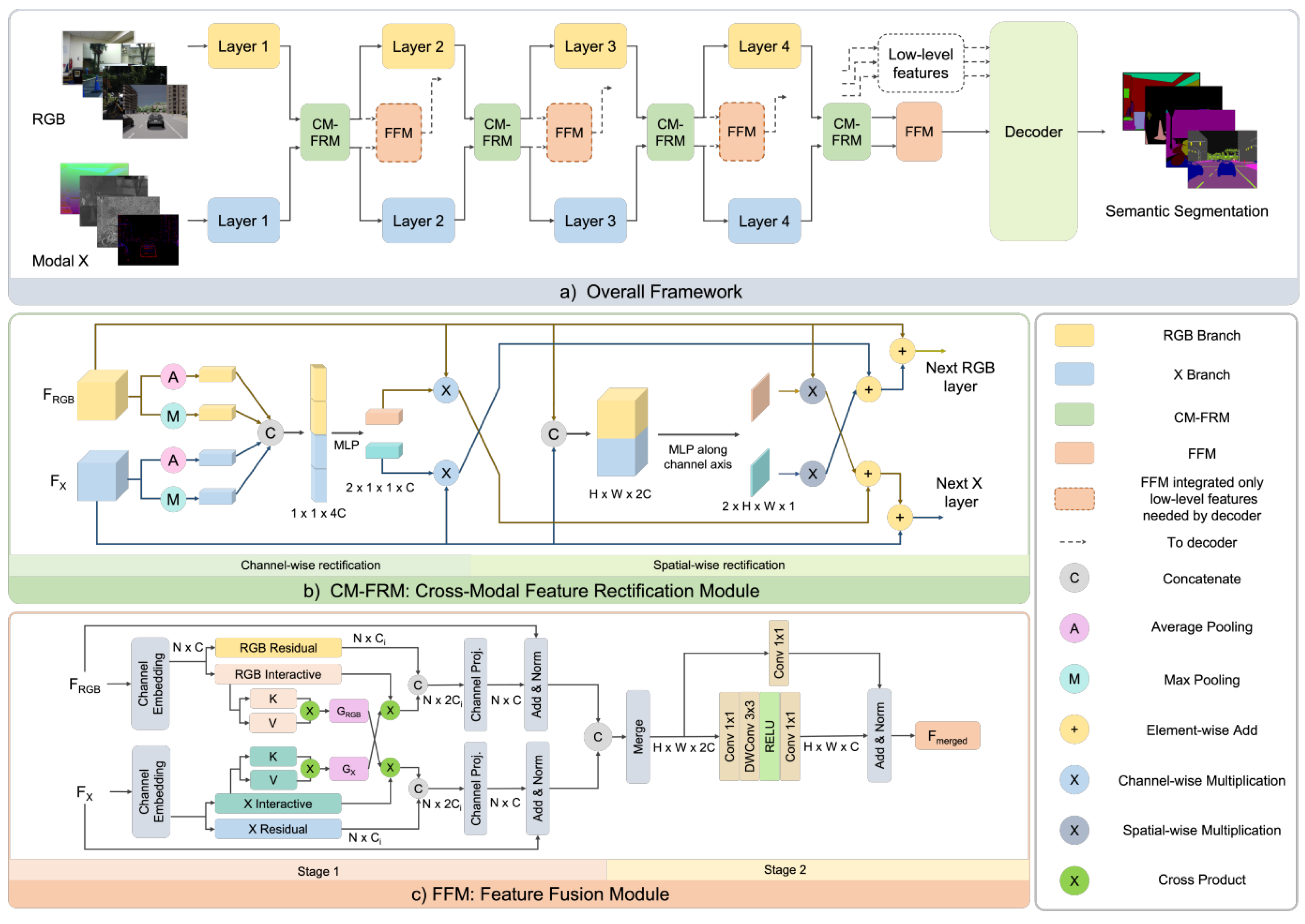
- Liu, H.; Zhang, J.; Yang, K.; Hu, X.; Stiefelhagen, R. CMX: Cross-Modal Fusion for RGB-X Semantic Segmentation with Transformers. arXiv 2022, arXiv:2203.04838. [Google Scholar]
- Wang, Y.; Sun, F.; Lu, M.; Yao, A. Learning deep multimodal feature representation with asymmetric multi-layer fusion. In Proceedings of the 28th ACM International Conference on Multimedia, Seattle, WA, USA, 12–16 October 2020; pp. 3902–3910. [Google Scholar]
- Chen, X.; Lin, K.Y.; Wang, J.; Wu, W.; Qian, C.; Li, H.; Zeng, G. Bi-directional cross-modality feature propagation with separation-and-aggregation gate for RGB-D semantic segmentation. In Proceedings of the European Conference on Computer Vision, Glasgow, UK, 23–28 August 2020; pp. 561–577. [Google Scholar]
- Seichter, D.; Köhler, M.; Lewandowski, B.; Wengefeld, T.; Gross, H.M. Efficient rgb-d semantic segmentation for indoor scene analysis. In Proceedings of the 2021 IEEE International Conference on Robotics and Automation (ICRA), Xi’an, China, 30 May–5 June 2021; pp. 13525–13531. [Google Scholar]
- Kong, S.; Fowlkes, C.C. Recurrent scene parsing with perspective understanding in the loop. In Proceedings of the IEEE Conference on Computer Vision and Pattern Recognition, Salt Lake City, UT, USA, 18–23 June 2018; pp. 956–965. [Google Scholar]
- Deng, L.; Yang, M.; Li, T.; He, Y.; Wang, C. RFBNet: Deep multimodal networks with residual fusion blocks for RGB-D semantic segmentation. arXiv 2019, arXiv:1907.00135. [Google Scholar]
- Valada, A.; Vertens, J.; Dhall, A.; Burgard, W. Adapnet: Adaptive semantic segmentation in adverse environmental conditions. In Proceedings of the 2017 IEEE International Conference on Robotics and Automation (ICRA), Singapore, 29 May–3 June 2017; pp. 4644–4651. [Google Scholar]
- Sun, Y.; Zuo, W.; Liu, M. Rtfnet: Rgb-thermal fusion network for semantic segmentation of urban scenes. IEEE Robot. Autom. Lett. 2019, 4, 2576–2583. [Google Scholar] [CrossRef]
- Zhuang, Z.; Li, R.; Jia, K.; Wang, Q.; Li, Y.; Tan, M. Perception-aware Multi-sensor Fusion for 3D LiDAR Semantic Segmentation. In Proceedings of the IEEE/CVF International Conference on Computer Vision, Montreal, QC, Canada, 10–17 October 2021; pp. 16280–16290. [Google Scholar]
- Rashed, H.; El Sallab, A.; Yogamani, S.; ElHelw, M. Motion and depth augmented semantic segmentation for autonomous navigation. In Proceedings of the IEEE/CVF Conference on Computer Vision and Pattern Recognition Workshops, Long Beach, CA, USA, 15–20 June 2019. [Google Scholar]
- Zhang, Y.; Morel, O.; Seulin, R.; Mériaudeau, F.; Sidibé, D. A central multimodal fusion framework for outdoor scene image segmentation. Multimed. Tools Appl. 2022, 81, 12047–12060. [Google Scholar] [CrossRef]
- Yi, S.; Li, J.; Liu, X.; Yuan, X. CCAFFMNet: Dual-spectral semantic segmentation network with channel-coordinate attention feature fusion module. Neurocomputing 2022, 482, 236–251. [Google Scholar] [CrossRef]
- Frigo, O.; Martin-Gaffé, L.; Wacongne, C. DooDLeNet: Double DeepLab Enhanced Feature Fusion for Thermal-color Semantic Segmentation. In Proceedings of the 2022 IEEE Computer Society Conference on Computer Vision and Pattern Recognition (CVPR), New Orleans, LO, USA, 19–24 June 2022; pp. 3021–3029. [Google Scholar]
- Zhou, W.; Liu, J.; Lei, J.; Yu, L.; Hwang, J.N. GMNet: Graded-Feature Multilabel-Learning Network for RGB-Thermal Urban Scene Semantic Segmentation. IEEE Trans. Image Process. 2021, 30, 7790–7802. [Google Scholar] [CrossRef]
- Deng, F.; Feng, H.; Liang, M.; Wang, H.; Yang, Y.; Gao, Y.; Chen, J.; Hu, J.; Guo, X.; Lam, T.L. FEANet: Feature-Enhanced Attention Network for RGB-Thermal Real-time Semantic Segmentation. In Proceedings of the 2021 IEEE/RSJ International Conference on Intelligent Robots and Systems (IROS), Prague, Czech Republic, 27 September–1 October 2021; pp. 4467–4473. [Google Scholar] [CrossRef]
- Zhou, W.; Dong, S.; Xu, C.; Qian, Y. Edge-aware Guidance Fusion Network for RGB Thermal Scene Parsing. In Proceedings of the Thirty-Sixth AAAI Conference on Artificial Intelligence, Washington, DC, USA, 7–14 February 2022; pp. 3571–3579. [Google Scholar]
- Zhang, Q.; Zhao, S.; Luo, Y.; Zhang, D.; Huang, N.; Han, J. ABMDRNet: Adaptive-weighted Bi-directional Modality Difference Reduction Network for RGB-T Semantic Segmentation. In Proceedings of the IEEE/CVF Conference on Computer Vision and Pattern Recognition, Nashville, TN, USA, 20–25 June 2021; pp. 2633–2642. [Google Scholar]
- Xu, J.; Lu, K.; Wang, H. Attention fusion network for multi-spectral semantic segmentation. Pattern Recognit. Lett. 2021, 146, 179–184. [Google Scholar] [CrossRef]
- Sun, Y.; Zuo, W.; Yun, P.; Wang, H.; Liu, M. FuseSeg: Semantic segmentation of urban scenes based on RGB and thermal data fusion. IEEE Trans. Autom. Sci. Eng. 2020, 18, 1000–1011. [Google Scholar] [CrossRef]
- Krispel, G.; Opitz, M.; Waltner, G.; Possegger, H.; Bischof, H. Fuseseg: Lidar point cloud segmentation fusing multi-modal data. arXiv 2020, arXiv:1912.08487. [Google Scholar] [CrossRef]
- El Madawi, K.; Rashed, H.; El Sallab, A.; Nasr, O.; Kamel, H.; Yogamani, S. Rgb and lidar fusion based 3d semantic segmentation for autonomous driving. In Proceedings of the 2019 IEEE Intelligent Transportation Systems Conference (ITSC), Auckland, New Zealand, 27–30 October 2019; pp. 7–12. [Google Scholar]
- Wang, W.; Neumann, U. Depth-aware CNN for RGB-D Segmentation. In Proceedings of the European Conference on Computer Vision (ECCV), Munich, Germany, 8–14 September 2018; pp. 135–150. [Google Scholar]
- Jaritz, M.; Vu, T.H.; Charette, R.d.; Wirbel, E.; Pérez, P. xmuda: Cross-modal unsupervised domain adaptation for 3d semantic segmentation. In Proceedings of the IEEE/CVF Conference on Computer Vision and Pattern Recognition, Seattle, WA, USA, 13–19 June 2020; pp. 12605–12614. [Google Scholar]
- Chollet, F. Xception: Deep Learning with Depthwise Separable Convolutions. In Proceedings of the 2018 IEEE/CVF Conference on Computer Vision and Pattern Recognition, Honolulu, HI, USA, 21–26 July 2017; pp. 1251–1258. [Google Scholar] [CrossRef] [Green Version]
- Zhao, H.; Qi, X.; Shen, X.; Shi, J.; Jia, J. ICNet for Real-Time Semantic Segmentation on High-Resolution Images. In Proceedings of the ECCV, Munich, Germany, 8–14 September 2018. [Google Scholar]
- Iandola, F.N.; Moskewicz, M.W.; Ashraf, K.; Han, S.; Dally, W.J.; Keutzer, K. SqueezeNet: AlexNet-level accuracy with 50x fewer parameters and <1 MB model size. arXiv 2016, arXiv:1602.07360. [Google Scholar]
- Graham, B.; Engelcke, M.; Maaten, L.V.D. 3D Semantic Segmentation with Submanifold Sparse Convolutional Networks. In Proceedings of the 2018 IEEE/CVF Conference on Computer Vision and Pattern Recognition, Salt Lake City, UT, USA, 8–23 June 2018; pp. 9224–9232. [Google Scholar] [CrossRef] [Green Version]
- Xie, S.; Girshick, R.; Dollár, P.; Tu, Z.; He, K. Aggregated Residual Transformations for Deep Neural Networks. In Proceedings of the 2018 IEEE/CVF Conference on Computer Vision and Pattern Recognition, Honolulu, HI, USA, 21–26 July 2017; pp. 1492–1500. [Google Scholar] [CrossRef] [Green Version]
- Huang, G.; Liu, Z.; Van Der Maaten, L.; Weinberger, K.Q. Densely connected convolutional networks. In Proceedings of the 2018 IEEE/CVF Conference on Computer Vision and Pattern Recognition, Honolulu, HI, USA, 21–26 July 2017; pp. 4700–4708. [Google Scholar] [CrossRef] [Green Version]
- Couprie, C.; Farabet, C.; Najman, L.; LeCun, Y. Indoor semantic segmentation using depth information. arXiv 2013, arXiv:1301.3572. [Google Scholar]
- Pagnutti, G.; Minto, L.; Zanuttigh, P. Segmentation and semantic labelling of RGBD data with convolutional neural networks and surface fitting. IET Comput. Vis. 2017, 11, 633–642. [Google Scholar] [CrossRef] [Green Version]
- Hu, J.; Shen, L.; Sun, G. Squeeze-and-Excitation Networks. In Proceedings of the 2018 IEEE/CVF Conference on Computer Vision and Pattern Recognition, Salt Lake City, UT, USA, 8–23 June 2018; pp. 7132–7141. [Google Scholar] [CrossRef] [Green Version]
- Su, H.; Maji, S.; Kalogerakis, E.; Learned-Miller, E. Multi-view convolutional neural networks for 3d shape recognition. In Proceedings of the IEEE International Conference on Computer Vision, Santiago, Chile, 11–18 December 2015; pp. 945–953. [Google Scholar]
- Chiang, H.Y.; Lin, Y.L.; Liu, Y.C.; Hsu, W.H. A unified point-based framework for 3d segmentation. In Proceedings of the 2019 International Conference on 3D Vision (3DV), Québec City, QC, Canada, 16–19 September 2019; pp. 155–163. [Google Scholar]
- Jaritz, M.; Gu, J.; Su, H. Multi-view pointnet for 3d scene understanding. In Proceedings of the IEEE/CVF International Conference on Computer Vision Workshops, Seoul, Korea, 27–28 October 2019. [Google Scholar]
- Ronneberger, O.; Fischer, P.; Brox, T. U-net: Convolutional networks for biomedical image segmentation. In Proceedings of the International Conference on Medical Image Computing and Computer-Assisted Intervention, Munich, Germany, 5–9 October 2015; pp. 234–241. [Google Scholar]
- Liu, W.; Luo, Z.; Cai, Y.; Yu, Y.; Ke, Y.; Junior, J.M.; Gonçalves, W.N.; Li, J. Adversarial unsupervised domain adaptation for 3D semantic segmentation with multi-modal learning. ISPRS J. Photogramm. Remote Sens. 2021, 176, 211–221. [Google Scholar] [CrossRef]


| Sensor | Range | Sparsity | Robustness | Direct Sun Perf. | Night Perf. | Cost |
|---|---|---|---|---|---|---|
| Passive Stereo | Far | Dense | Low | Medium | Low | Very Low |
| Active Stereo | Medium | Dense | Medium | Medium | Good | Low |
| Matricial ToF | Medium | Dense | High | Low | Good | Medium |
| LiDAR | Far | Sparse | High | Good | Good | High |
| RADAR | Far | Very Sparse | Medium | Good | Good | Low |
 indicates that single views of the 3D scene are labeled, * indicates variability with no control or categorization. The table is color-coded to indicate the scenarios present in each dataset:
  Driving,
  Exterior,
  In/Out,
  Interior.
indicates that single views of the 3D scene are labeled, * indicates variability with no control or categorization. The table is color-coded to indicate the scenarios present in each dataset: Driving, Exterior, In/Out, Interior.
Interior.
indicates that single views of the 3D scene are labeled, * indicates variability with no control or categorization. The table is color-coded to indicate the scenarios present in each dataset: Driving, Exterior, In/Out, Interior.| Metadata | Sensors | Diversity | Labels | Size | |||||||||||||||
|---|---|---|---|---|---|---|---|---|---|---|---|---|---|---|---|---|---|---|---|
| Name | Created | Update | Type | Cameras | LiDARs | Stereo | GT Depths | RADARs | IMU | Daytime | Seasons | Location | Weather | Env. Control | Sem Seg | Bboxes | Opt. Flow | Sequences | Labeled Sampl. |
| KITTI [8,65,66,67] | 2012 | 2015 | R | 2G/2C | 1 | 2 | - | - | + | - | - | - | - | - | - | + | - | 1(6 h) | 200 |
| Cityscapes [68] | 2016 | 2016 | R | 2C | - | 1 | - | - | + | - | - | 27C † | - | - | + | - | - | - | 5000 |
| Lost and found [69] | 2016 | 2016 | R | 2C | - | 1 | - | - | - | - | - | - | - | - | + | - | - | 112 | 2104 |
| Synthia [70,71,72] | 2016 | 2019 | S | 1C | - | - | 1 | - | - | DS | + | - | 2 | - | + | - | - | - | 9400 |
| Virtual KITTI [73,74] | 2016 | 2020 | S | 2C | - | 1 | 1 | - | + | MDS | - | - | 4 | + | + | + | + | 35 | 17k |
| MSSSD/MF [75] | 2017 | 2017 | R | 1C/1T | - | - | - | - | - | DN | - | - | - | - | + | - | - | - | 1569 |
| RoadScene-Seg [76] | 2018 | 2018 | R | 1C/1T | - | - | - | - | - | DN | - | - | - | - | - | - | - | - | 221 |
| AtUlm [77] | 2019 | 2019 | R | 1G | 4 | - | - | - | - | - | - | - | - | - | + | - | - | - | 1446 |
| nuScenes [78] | 2019 | 2020 | R | 6C | 1 | 1 | - | 5 | + | - | - | T | - | - | + | + | - | - | 40k |
| SemanticKITTI [35] | 2019 | 2021 | R | - | 1 | - | - | - | - | - | - | - | - | - | + | - | - | 22 | 43,552 |
| ZJU [79] | 2019 | 2019 | R | 2C/1FE/1P | - | 1 | - | - | - | DN | - | - | - | - | - | - | - | - | 3400 |
| A2D2 [80] | 2020 | 2020 | R | 6C | 5 | - | - | - | + | - | - | - | - | - | + | + | - | - | 41,280 |
| ApolloScape [81] | 2020 | 2020 | R | 6C | 2 | 1 | - | - | + | * | - | 4R † | * | - | + | + | - | - | 140k |
| DDAD [82] | 2020 | 2020 | R | 6C | 4 | - | - | - | - | - | - | 2R | - | - | - | - | - | - | 16,600 |
| KITTI 360 [83] | 2021 | 2021 | R | 2C/2FE | 1 | 1 | - | - | + | - | - | - | - | - | + | + | - | - | 78k |
| WoodScape [84] | 2021 | 2021 | R | 4FE | 1 | - | - | - | + | - | - | 10C | - | - | + | + | - | - | 10k |
| EventScape [85] | 2021 | 2021 | S | 1C/1E | - | - | 1 | - | + | - | - | 4C | - | - | + | + | - | 743(2 h) | - |
| SELMA [39] | 2022 | 2022 | S | 8C | 3 | 3 | 7 | - | - | DSN | - | 7C | 9 | + | + | + | - | - | 31k×27 |
| Freiburg Forest [86] | 2016 | 2016 | R | 2C/1MS | - | 1 | - | - | - | - | - | - | - | - | + | - | - | - | 336 |
| POLABOT [87] | 2019 | 2019 | R | 2C/1P/1MS | - | 1 | - | - | - | - | - | - | - | - | + | - | - | - | 175 |
| SRM [88] | 2021 | 2021 | R | 1C/1T | - | - | - | - | - | - | - | - | 2 | - | + | - | - | - | 2458 |
| SSW [88] | 2021 | 2021 | R | 1C/1T | - | - | - | - | - | - | - | - | 2 | - | + | - | - | - | 1571 |
| MVSEC [89] | 2018 | 2018 | R | 2G/2E | 1 | 1 | - | - | + | DN | - | IO | - | - | - | - | - | 14(1 h) | - |
| PST900 [90] | 2019 | 2019 | R | 2C/1T | - | 1 | - | - | - | - | - | IO | - | - | + | - | - | - | 4316 |
| NYU-depth-v2 [91] | 2012 | 2012 | R | 1C + 1D | - | - | 1 | - | - | - | - | - | - | - | + | - | - | - | 1449 |
| SUN-RGBD [92] | 2015 | 2015 | R | 1C + 1D | - | - | 1 | - | - | - | - | - | - | - | + | - | - | - | 10k |
| 2D-3D-S [93] | 2017 | 2017 | R | 1C + 1D | - | - | 1 | - | - | - | - | - | - | - | + | - | - | - | 270 |
| ScanNet [94] | 2017 | 2018 | R | 1C + 1D | - | - | 1 | - | - | - | - | - | - | - | + | - | - | - | 1513 |
| Taskonomy [95] | 2018 | 2018 | R | 1C + 1D | - | - | 1 | - | - | - | - | - | - | - | ∼ | - | - | - | 4 m |
| Metadata | Fusion Approach | Fusion Architecture | ||||||||||||
|---|---|---|---|---|---|---|---|---|---|---|---|---|---|---|
| Name | Year | Dataset(s) | Modality(ies) | + | × | ⨀ | Ad-Hoc Block | Ad-Hoc Loss | Multi-Task | Location | Direction | Parallel Branches | Skip Connections | Multi-Level Fusion |
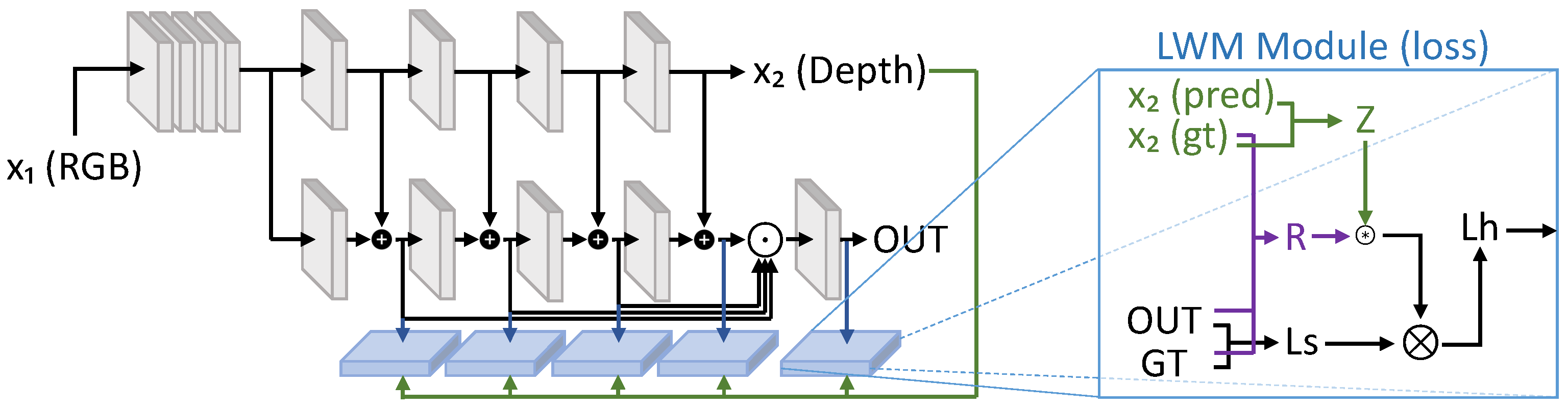
| LWM [97] | 2021 | [68,91,92] | DmDe | + | - | + | - | + | + | D | D/C | 2 | + | + |
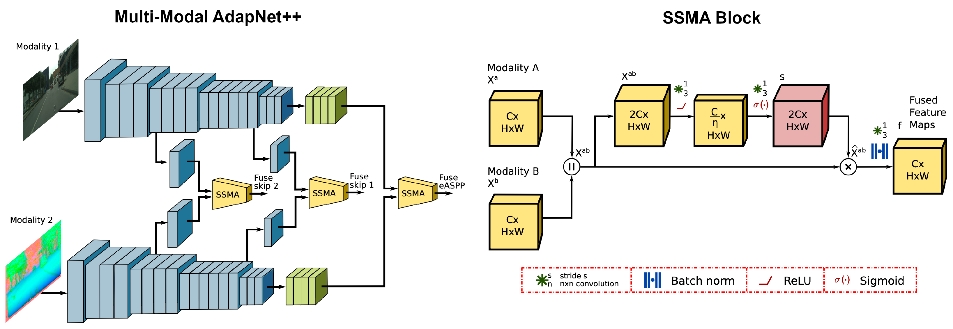
| SSMA [98] | 2019 | [68,70,86,92,94] | DmDhT | - | + | + | + | + | - | E | D | 2 | + | + |
| CMX [99] | 2022 | [68,75,79,85,91,92,93,94] | EDhLpT | + | + | - | + | - | - | E | D/B | 2 | + | + |
| AsymFusion [100] | 2021 | [68,91,95] | Dm | + | - | - | + | - | - | E | B | 2 | - | + |
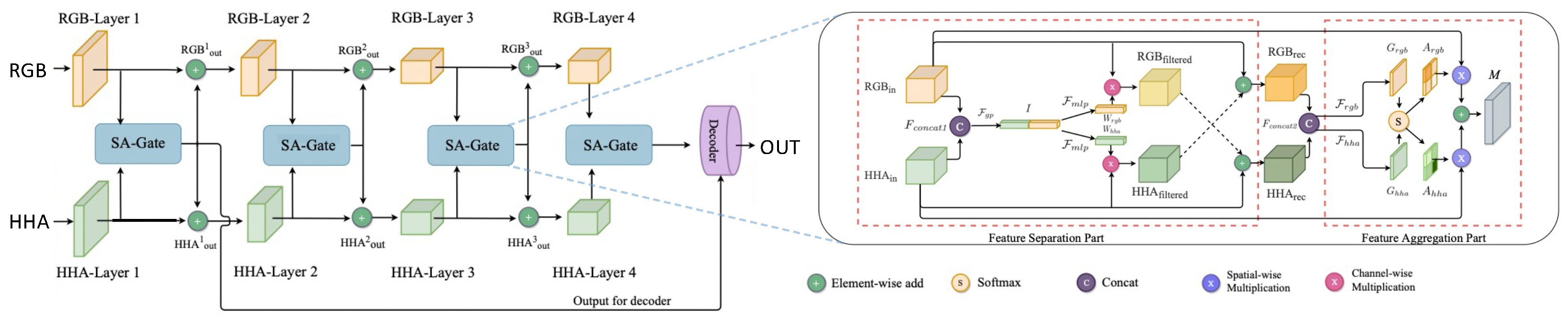
| SA-Gate [101] | 2020 | [68,91] | Dh | + | - | + | + | - | - | E | B | 2 | + | + |
| ESANet [102] | 2021 | [68,91,92] | Dm | + | - | - | - | - | - | E | C | 2 | + | + |
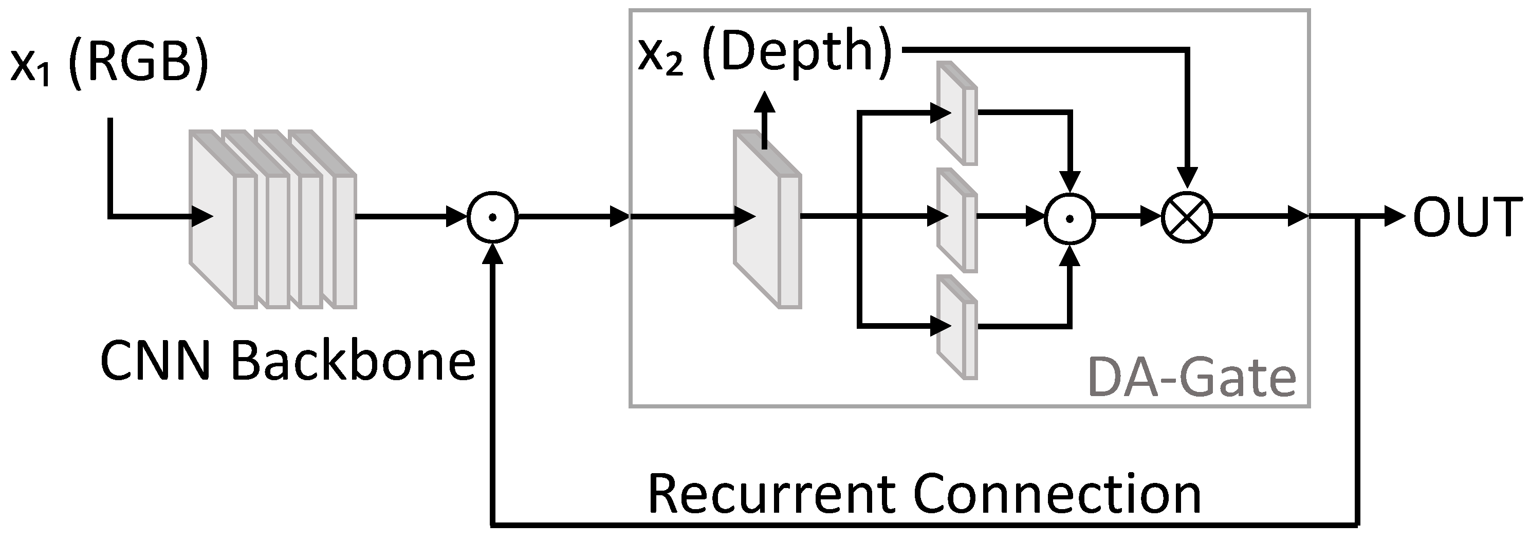
| DA-Gate [103] | 2018 | [68,91,92,93] | DmDe | - | - | - | - | + | - | N/A | N/A | 1 | - | - |
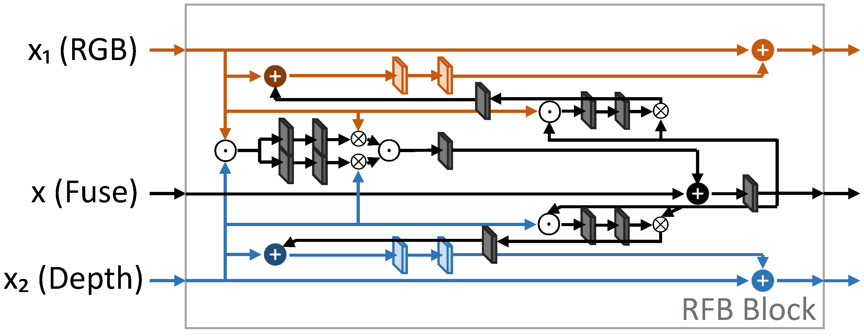
| RFBNet [104] | 2019 | [68,94] | Dh | + | + | + | + | - | - | E | B | 2 | - | + |
| MMSFB-snow [88] | 2021 | [68,70,88] | DmT | - | - | + | + | - | - | E | D | 2 | + | + |
| AdapNet [105] | 2017 | [68,70,86] | DmT | + | + | - | + | - | - | D | D | 2 | - | - |
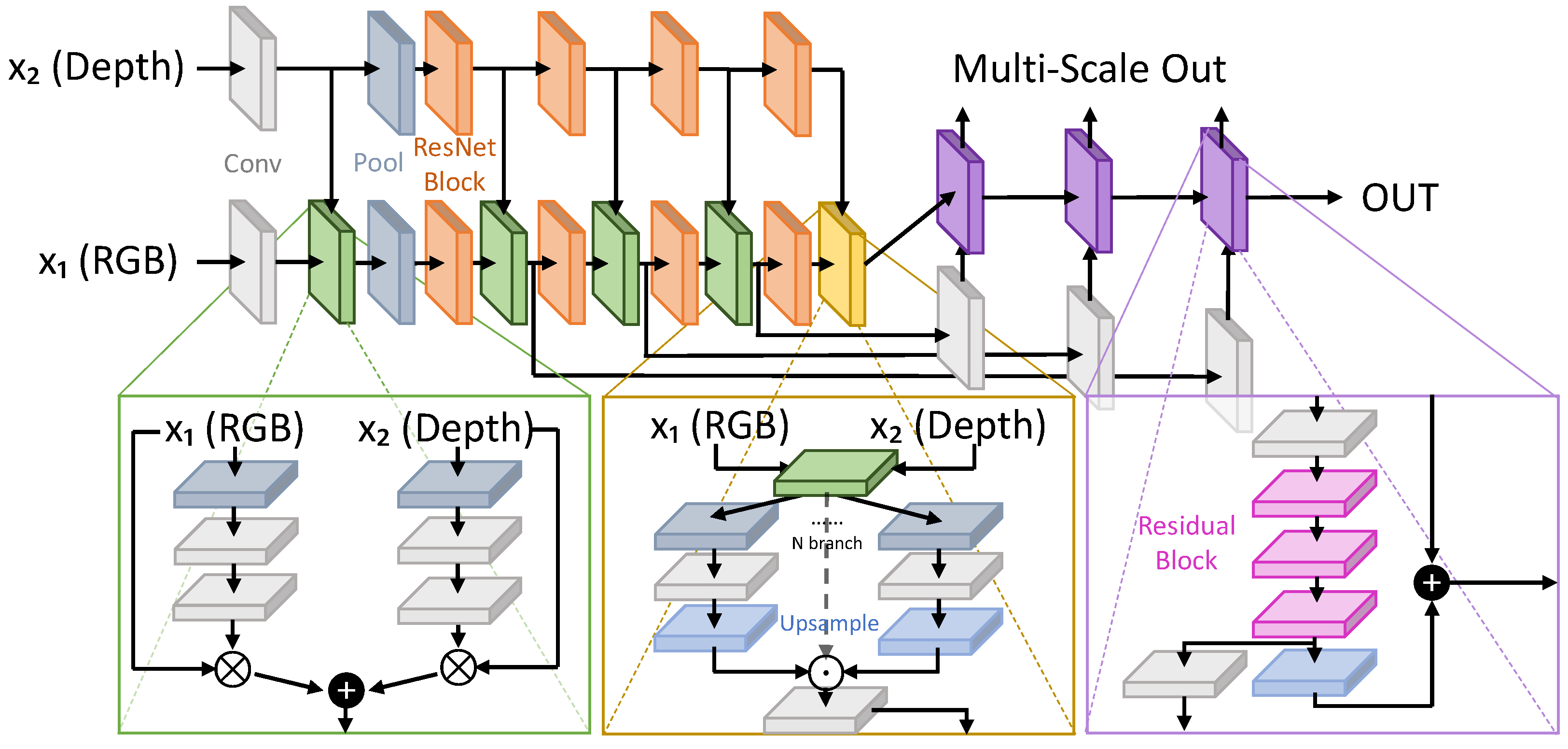
| RFNet [106] | 2020 | [68,69] | Dm | + | - | - | + | - | - | E | C | 2 | + | + |
| RSSAWC [77] | 2019 | [68,77] | DmLi | + | - | + | - | - | - | E | D | 2 | - | - |
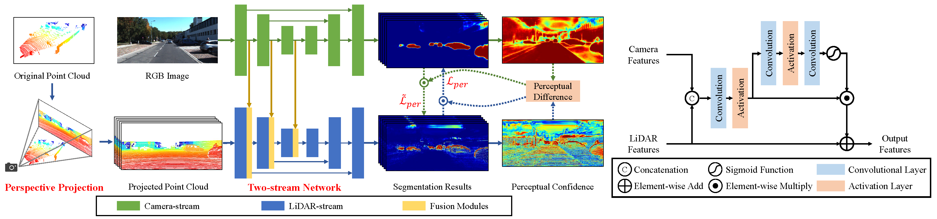
| PMF [107] | 2021 | [35,78] | Li | + | + | + | + | + | - | E | M | 2 | + | + |
| MDASS [108] | 2019 | [68,73] | DmF | + | - | - | - | - | - | E | D | 2/3 | + | + |
| CMFnet [109] | 2021 | [68,87] | DmLp | - | + | + | - | - | - | E | D/B | 3+ | - | + |
| CCAFFMNet [110] | 2021 | [75,76] | T | - | - | + | + | - | - | E | C | 2 | + | + |
| DooDLeNet [111] | 2022 | [75] | T | - | + | + | - | - | - | E | D | 2 | + | + |
| GMNet [112] | 2021 | [75,90] | T | + | + | - | + | - | + | E | D | 2 | + | + |
| FEANet [113] | 2021 | [75] | T | + | + | - | - | - | - | E | C | 2 | - | + |
| EGFNet [114] | 2021 | [75,90] | T | + | + | + | + | - | - | E | D | 2 | - | + |
| ABMDRNet [115] | 2021 | [75] | T | + | + | + | + | + | + | E | D | 2 | - | + |
| AFNet [116] | 2021 | [75] | T | + | + | - | + | - | - | E | D | 2 | - | - |
| FuseSeg-Thermal [117] | 2021 | [75] | T | + | - | + | - | - | - | E | C | 2 | + | + |
| RTFNet [106] | 2019 | [75] | T | + | - | - | - | - | - | E | C | 2 | - | + |
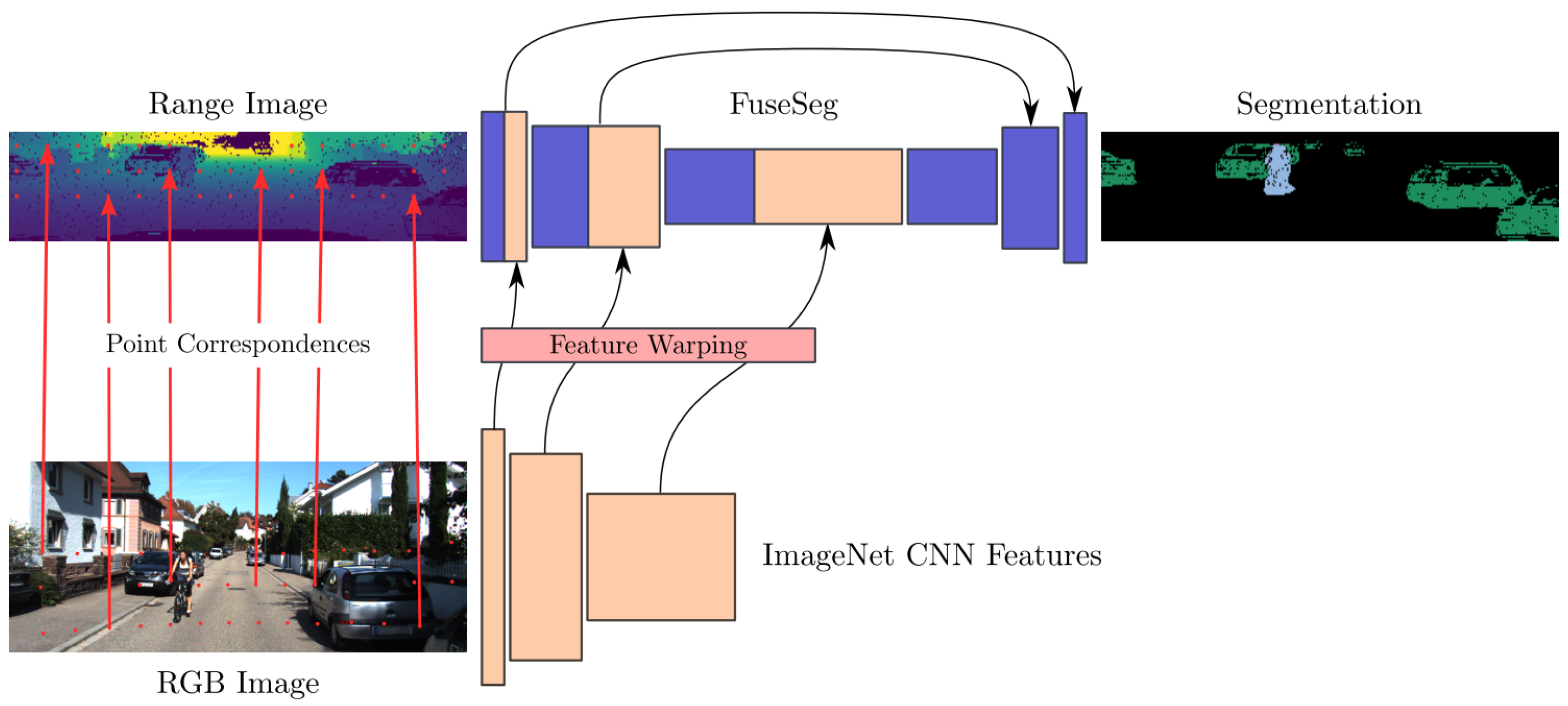
| FuseSeg-LiDAR [118] | 2020 | [8] | LsLi | - | - | + | - | - | - | E | M | 2 | + | + |
| RaLF3D [119] | 2019 | [8] | LsLi | + | - | + | - | - | - | E | D | 2 | + | + |
| DACNN [120] | 2018 | [91,92,93] | DmDh | + | - | - | - | - | - | E | D | 2 | - | - |
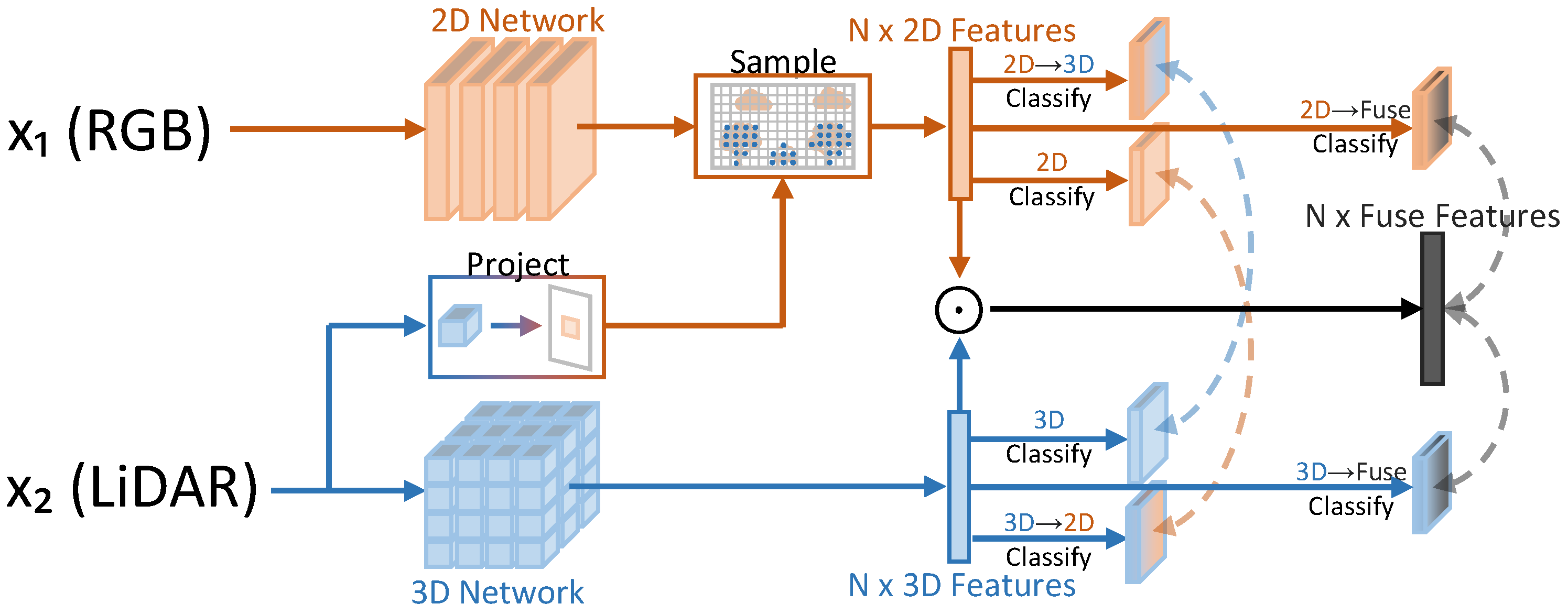
| xMUDA [121] | 2020 | [35,78,80] | Li | - | - | + | - | + | + | D | D | 2 | - | + |
| Name | Backbone | mIoU |
|---|---|---|
| (a) Cityscapes dataset (2.5D SS). | ||
| LWM [97] | ResNet101 [16] | 83.4 |
| SSMA [98] | ResNet50 [16] | 83.29 |
| CMX [99] | MiT-B4 [27] | 82.6 |
| AsymFusion [100] | Xception65 [122] | 82.1 |
| SA-Gate [101] | ResNet101 [16] | 81.7 |
| ESANet [102] | ResNet34 [16] | 80.09 |
| DA-Gate [103] | ResNet101 [16] | 75.3 |
| RFBNet [104] | ResNet50 [16] | 74.8 |
| MMSFB-snow [88] | ResNet50 [16] | 73.8 |
| AdapNet [105] | AdapNet [105] | 71.72 |
| RFNet [106] | ResNet18 [16] | 69.37 |
| RSSAWC [77] | ICNet [123] | 65.09 |
| MDASS [108] | VGG16 [15] | 63.13 |
| CMFnet [109] | VGG16 [15] | 58.97 |
| (b) KITTI dataset (2D + 3D SS). | ||
| PMF [107] | ResNet34 [16] | 63.9 |
| FuseSeg-LiDAR [118] | SqueezeNet [124] | 52.1 |
| RaLF3D [119] | SqueezeSeg [33] | 37.8 |
| xMUDA [121] | SparseConvNet3D [125] ResNet34 [16] | 49.1 |
| (c) MSSSD/MF dataset (RGB + Thermal SS). | ||
| CMX [99] | MiT-B4 [27] | 59.7 |
| CCAFFMNet [110] | ResNeXt50 [126] | 58.2 |
| DooDLeNet [111] | ResNet101 [16] | 57.3 |
| GMNet [112] | ResNet50 [16] | 57.3 |
| FEANet [113] | ResNet101 [16] | 55.3 |
| EGFNet [114] | ResNet152 [16] | 54.8 |
| ABMDRNet [115] | ResNet50 [16] | 54.8 |
| AFNet [116] | ResNet50 [16] | 54.6 |
| FuseSeg-Thermal [117] | DenseNet161 [127] | 54.5 |
| RTFNet [106] | ResNet152 [16] | 53.2 |
Publisher’s Note: MDPI stays neutral with regard to jurisdictional claims in published maps and institutional affiliations. |
© 2022 by the authors. Licensee MDPI, Basel, Switzerland. This article is an open access article distributed under the terms and conditions of the Creative Commons Attribution (CC BY) license (https://creativecommons.org/licenses/by/4.0/).
Share and Cite
Rizzoli, G.; Barbato, F.; Zanuttigh, P. Multimodal Semantic Segmentation in Autonomous Driving: A Review of Current Approaches and Future Perspectives. Technologies 2022, 10, 90. https://doi.org/10.3390/technologies10040090
Rizzoli G, Barbato F, Zanuttigh P. Multimodal Semantic Segmentation in Autonomous Driving: A Review of Current Approaches and Future Perspectives. Technologies. 2022; 10(4):90. https://doi.org/10.3390/technologies10040090
Chicago/Turabian StyleRizzoli, Giulia, Francesco Barbato, and Pietro Zanuttigh. 2022. "Multimodal Semantic Segmentation in Autonomous Driving: A Review of Current Approaches and Future Perspectives" Technologies 10, no. 4: 90. https://doi.org/10.3390/technologies10040090
APA StyleRizzoli, G., Barbato, F., & Zanuttigh, P. (2022). Multimodal Semantic Segmentation in Autonomous Driving: A Review of Current Approaches and Future Perspectives. Technologies, 10(4), 90. https://doi.org/10.3390/technologies10040090