Efficient Stochastic Computing FIR Filtering Using Sigma-Delta Modulated Signals

Abstract

This work presents a soft-filtering digital signal processing architecture based on sigma-delta modulators and stochastic computing. A sigma-delta modulator converts the input high-resolution signal to a single-bit stream enabling filtering structures to be realized using stochastic computing’s negligible-area multipliers. Simulation in the spectral domain demonstrates the filter’s proper operation and its roll-off behavior, as well as the signal-to-noise ratio improvement using the sigma-delta modulator, compared to typical stochastic computing filter realizations. The proposed architecture’s hardware advantages are showcased with synthesis results for two FIR filters using FPGA and synopsys tools, while comparisons with standard stochastic computing-based hardware realizations, as well as with conventional binary ones, demonstrate its efficacy.

1. Introduction

Modern digital signal processing (DSP) blocks are characterized by hardware efficiency and high-performance computations [1,2]. On the other hand, standard binary computing methods impose constraints on their design specifications, namely power, area, and energy, which are continuously increasing given the rise of hardware-taxing emerging applications [2]. To this end, unconventional computing paradigms are explored as an alternative to the binary one, with stochastic computing (SC) being an attractive approach [3,4,5,6].

SC represents real-valued numbers in the form of stochastic sequences [7]. Encoding the information in such a way makes its processing resilient to soft errors originating from noisy sources [3,8], for instance bit-flips, which is prohibitive in the case of the binary arithmetic. Furthermore, SC’s bit-processing nature allows for the realization of fundamental arithmetic operations as well as highly-complex functions using a few standard logic gates and cells, thereby reducing the hardware requirements when compared to their binary counterparts [3,4,9,10,11,12].

The advantages of SC favor the design of several applications, especially the ones in which parallelization is necessary. These include neural networks [13,14,15,16,17,18,19], digital image processing [20,21,22,23,24], soft-polynomial solving and filtering [25,26,27,28,29,30], modern error coding and decoding, etc. [31]. Focusing on digital filters, SC-based implementations of the standard Nyquist-rate ones are proven to be hardware-efficient [25,27,28,29,30]. Their key advantage lies in the multiplication process; instead of using the area-demanding binary multipliers, SC exploits simple XNOR gates and MUXs to realize the multiplication and addition parts, respectively, improving the area occupied by the intensive multiply-and-add operations.

Although the SC filters realized using the methods considered in [27,28,29,30] reduce the hardware resources when compared to the standard binary approach, they are also limited in their spectral characteristics. Specifically, their performance is affected by two factors: (1) the length of the stochastic sequence required to process a single sample, which is SC’s essential design trade-off, and (2) the noise introduced from the binary-to-stochastic converters used to generate the input signal and the filter’s coefficients.

A well-known method to reduce the noise floor and improve the spectral characteristics of a quantized signal is to use sigma-delta modulators (SDMs) [32,33,34]. They convert a high-resolution signal (several bits) into a lower-bit one by employing the technique of oversampling; the input signal is sampled at a frequency much higher than the Nyquist, thus reducing the noise in the desired frequency band of interest.

Motivated by the properties of SDMs, the use of a first-order SDM in FIR filtering was recently explored in [26]. It serves as a single-bit encoder of an input (quantized) signal, allowing for the SC-based FIR filter’s multipliers to be realized exclusively by simple logic gates. As such, the proposed SDM-SC architecture’s advantage is twofold; on one hand it offers improved signal-to-noise ratio (SNR), due to the SDM’s oversampling technique, which is not possible with conventional SC-based filtering; on the other hand, the SDM allows for the filtered signal to be encoded in time, therefore reducing the SC’s typical accuracy–latency trade-off as well as the power and energy consumed for this process.

We organize the remainder of the proposed work as follows. In Section 2, we provide a background on the stochastic numbers and their properties, as well as the operation of the first-order SDM. In Section 3, we review the prior work in SC-based FIR filter realizations and mathematically formulate their operation. In Section 4, we present the SDM-SC architecture and explain its principle operation through proper analysis. Section 5 includes experimental results with respect to (1) the SDM-SC’s architecture spectral characteristics and (2) comparisons with the SC literature as well as the conventional binary filters in SNR, FPGA synthesis results, and hardware resources in a 45 nm process. Finally, Section 6 provides the conclusion.

2. Stochastic Computing and Sigma-Delta Modulation Notation and Principle Operation

In this section, we provide a background on the generation of stochastic numbers and their manipulation using standard logic gates, as well as explain the operation of the first-order sigma-delta modulator.

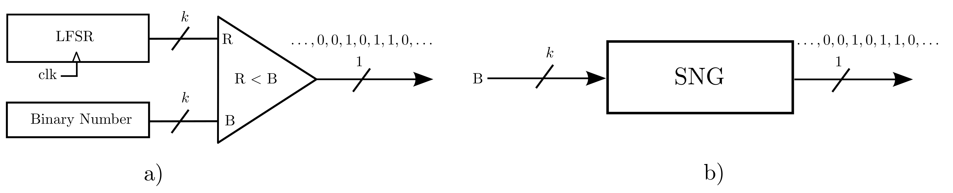
2.1. Stochastic Number Generation & Properties

The conversion of a binary number into a stochastic one is typically performed by the stochastic number generator (SNG), shown in Figure 1. Its operation is based upon the sampling on each clock cycle of a pseudo-random number generator uniformly distributed in ${\mathcal{R}}_s=\{0,1,\cdots ,2^k-1\}$, with the desired binary number $B\in [0,1]$ of the same bit length. Usually, the pseudo-random number source is implemented as a k-bit linear feedback shift register (LFSR), but note that other methods can also be used [35]. The bit generation is completed after $N=2^k$ clock cycles and corresponds to the length of the stochastic sequence.

Formally, the generated sequence of length N, ${\left\{X_n\right\}}_{n=1}^N$, where n denotes the current sample processed (or the current clock cycle), is assumed to be an independent and identically distributed (IID) Bernoulli sequence. Therefore, the generated stochastic number (SN) has probability defined as

$$\begin{array}{c}\hfill X\triangleq P(X_n=1)\end{array}$$

(1)

and mean value

$$\begin{array}{c}\hfill {\tilde{X}}_N\triangleq \frac{1}{N}\sum _{n=1}^N{X}_n.\end{array}$$

(2)

The SN’s mean value ${\tilde{X}}_N$ represents a non-negative number in $[0,1]$, known as unipolar format in SC, whereas to obtain a negative SN representation (known as bipolar format), the transformation $X\mapsto 2X-1$ is used, expanding the range of the SN to the interval $[-1,1]$. As expected, in both formats the sequence length N plays a critical role in the accuracy of the SN given the fact that it increases at the cost of additional clock cycles and is inversely proportional to $\sqrt{N}$ [36]. To further investigate the equivalent noise introduced by an SN, one can consider the noise figure (NF) [37] defined as

$$\begin{array}{c}\hfill NF\triangleq 10log10\left(\frac{P_S}{P_N}\right),\end{array}$$

(3)

where $P_S$ and $P_N$ are the average power and noise, respectively, of the generated SN.

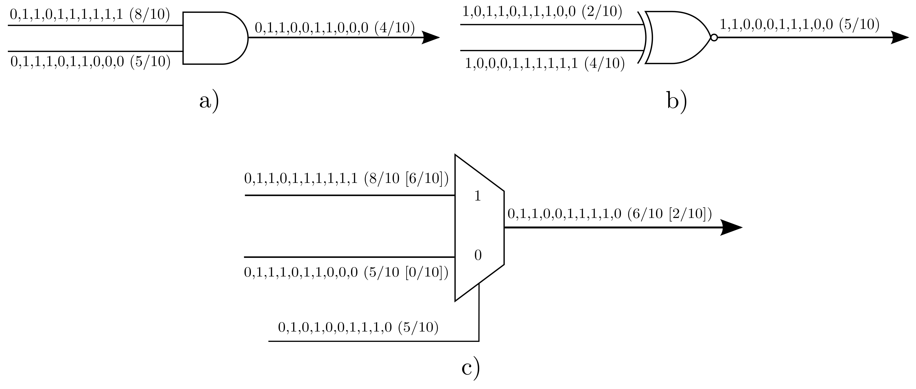
2.2. Mathematical Properties of Logic Gates in Stochastic Computing

Fundamental mathematical operations are supported in the context of SC and can be implemented by simple logical gates, according to the format used. For the following, we assume that ${\left\{X_n\right\}}_{n=1}^N$, ${\left\{Y_n\right\}}_{n=1}^N$ are stochastic sequences generated by different SNGs, to ensure independence among them, and ${\left\{H_n\right\}}_{n=1}^N$ is the result of their operation. We also note that whenever the bipolar format is required, the transformation $X\mapsto 2X-1$ is used.

• NOT Gate
  In unipolar format, the output of the NOT gate, $H_n=\mathrm{NOT}\left(X_n\right)$, complements the probability of the input,

  $$\begin{array}{c}\hfill H=P(H_n=1)=P(X_n=0)=1-P(X_n=1)=1-X,\end{array}$$

  (4)

  whereas in the bipolar format, it operates as a sign inverter.

  $$\begin{array}{c}\hfill H=P(H_n=1)=P(X_n=0)=1-P(X_n=1)=-X.\end{array}$$

  (5)
• AND Gate:
  The AND gate in unipolar format, $H_n=\mathrm{AND}(X_n,Y_n)$, performs multiplication.

  $$\begin{array}{c}\hfill H=P(H_n=1)=P(X_n=1,Y_n=1)=P(X_n=1)P(Y_n=1)=XY.\end{array}$$

  (6)
• XNOR Gate:
  The XNOR gate in bipolar format, $H_n=\mathrm{XNOR}(X_n,Y_n)$, performs multiplication.

  $$\begin{array}{cc}\hfill H& =P(H_n=1)=P(X_n=1,Y_n=1)+P(X_n=0,Y_n=0)\hfill \\ \hfill & =2P(X_n=1)P(Y_n=1)-P(X_n=1)-P(Y_n=1)+1\hfill \\ \hfill & =XY.\hfill \end{array}$$

  (7)
• Multiplexer
  Assuming an an IID control sequence ${\left\{C_n\right\}}_{n=1}^N$, the multiplexer (MUX), $H_n=\mathrm{MUX}(X_n,Y_n;C_n)$, is the standard way to perform scaled addition between two SN, regardless of the format used, and is given as

  $$\begin{array}{cc}\hfill H& =P(H_n=1)=P(X_n=1,C_n=1)+P(Y_n=1,C_n=0)\hfill \\ \hfill & =P(X_n=1)P(C_n=1)+P(Y_n=1)P(C_n=0)\hfill \\ \hfill & =XC+Y\overline{C}.\hfill \end{array}$$

  (8)
  Furthermore, if $P(C_n=1)=1/2$, the MUX operates as a scaling adder, i.e.,

  $$\begin{array}{cc}\hfill H& =P(H_n=1)=\frac{P(X_n=1)+P(Y_n=1)}{2}=\frac{X+Y}{2}.\hfill \end{array}$$

  (9)
  Stochastic subtraction, on the other hand, can only be realized in the bipolar format, using a NOT gate in one of the two inputs as

  $$\begin{array}{cc}\hfill H& =P(H_n=1)=\frac{P(X_n=1)+P(Y_n=0)}{2}=\frac{X-Y}{2}.\hfill \end{array}$$

  (10)

The operation of logic gates with specific interest is illustrated with an example in Figure 2.

2.3. Correlation in Stochastic Computing

The proper operation of SC processing elements is based upon the assumption that different SNGs are used as their input sequences. This is due to the fact that using the same initial seed in their LFSRs will cycle through the values in ${\mathcal{R}}_S$ simultaneously, thereby generating maximally correlated sequences (overlap of logic 1s) given the same binary number for conversion [38,39,40]. To provide better insight on the former, consider the case where the multiplication of two SNs is desired, i.e., $H=XY$, with $X=Y=0.6$. If SNGs with the same initial LFSR seed are used, then two identical sequences will be generated and their multiplication will result in $H=0.6$, instead of the correct one $H=0.36$. The same also happens when the LFSR is shared among the SNGs, without different seed initialization or proper use of delays. However, it has been shown that in certain cases, maximally correlated sequences can benefit specific applications [3,10], offering promising results.

A standard measure of correlation in SC is the stochastic computing correlation (SCC) [3,38]. For any two sequences $\left\{X_n\right\}$ and $\left\{Y_n\right\}$, then $\mathrm{SCC}(X_n,Y_n)$ is calculated as

$$SCC(X_n,Y_n)=\{\begin{array}{cc}{\displaystyle \frac{\mathbb{E}[X_n,Y_n]-\mathbb{E}\left[X_n\right]\mathbb{E}\left[Y_n\right]}{\min (\mathbb{E}\left[X_n\right],\mathbb{E}\left[Y_n\right])-\mathbb{E}\left[X_n\right]\mathbb{E}\left[Y_n\right]}},& \mathbb{E}[X_n,Y_n]>\mathbb{E}\left[X_n\right]\mathbb{E}\left[Y_n\right],\\ {\displaystyle \frac{\mathbb{E}[X_n,Y_n]-\mathbb{E}\left[X_n\right]\mathbb{E}\left[Y_n\right]}{\mathbb{E}\left[X_n\right]\mathbb{E}\left[Y_n\right]-\max (\mathbb{E}\left[X_n\right]+\mathbb{E}\left[Y_n\right]-1,0)},}& \mathrm{otherwise}\end{array}$$

(11)

taking values in $[-1,1]$, with $SCC(X_n,Y_n)=0$ corresponding to uncorrelated sequences. Note that SCC can also be used to measure the the auto-correlation of an output sequence, assuming the current output sample $H_n$ and its delayed version by $r>0$ samples $H_k$, with $k=n+r$, as $\mathrm{SCC}(H_n,H_k)$.

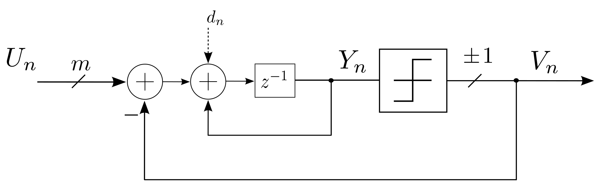
2.4. The First-Order Sigma-Delta Modulator

A Sigma-Delta Modulator (SDM) is typically used to convert a higher-resolution analog or digital signal into a lower-bit one. Its main advantage is the exploitation of the oversampling technique, which pushes the in-band quantization noise outside the input signal’s frequency band of interest. This is accomplished by sampling the input signal at a rate $f_s$ much higher than the Nyquist one. The oversampling ratio (OSR) is defined as

$$\begin{array}{c}\hfill OSR\triangleq \frac{f_s}{2f_B},\end{array}$$

(12)

where $f_B$ is the maximum input signal’s frequency. Oversampling has a direct impact on the spectral quality of the modulator and, more specifically, increasing the OSR leads to an improvement of the modulator’s signal-to-noise ratio (SNR) [34].

The first-order single-bit SDM is shown in Figure 3. It comprises an adder and an integrator, followed by a two-step quantizer block, $Q(·)$, which behaves as a nonlinear function as

$$\begin{array}{c}\hfill Q\left(Y_n\right)=\left\{\begin{array}{c}+1,Y_n\ge 0\hfill \\ -1,Y_n<0\hfill \end{array}\right..\end{array}$$

(13)

According to the SDM of Figure 3, the modulator’s input $U_n$, with n being the time index, is of m-bits length, whereas its output $V_n$ is single-bit $\pm 1$. Therefore, the behavior of the first-order SDM can be expressed as

$$\begin{array}{c}\hfill V_n=Q(Y_{n-1}+U_n-V_{n-1}).\end{array}$$

(14)

3. Prior Work in Stochastic Computing FIR Filters

For an arbitrary discrete-time signal $U_t$, $t=1,2,\cdots ,T$ and filter coefficients $w_m$, $m=1,2\cdots ,M$, an M-tap finite impulse response (FIR) filter is described as

$$Z_t=\sum _{m=0}^{M-1}{w}_m{V}_{t-m}={\mathbf{w}}^T\mathbf{V}.$$

(15)

where $\mathbf{w}=[w_0,w_1,\cdots ,w_{M-1}]\in {\mathbb{R}}^M$ and $\mathbf{V}=[V_t,V_{t-1},\cdots ,V_{t-M+1}]\in {\mathbb{R}}^M$. A straightforward realization of Equation (15), using SC techniques, requires $M-1$ XNOR gates for multiplication, as the values of $w_m,$ and $V_{t-m}$ might be negative, and an M-to-1 MUX for addition. However, this implementation leads to the downscaling of the output by a factor of $1/M$, which causes severe accuracy loss, especially when the filter’s order M is large.

To address this problem, a stochastic FIR filter that uses an MUX adder-tree was proposed in [41], and is based on the inner-product processing unit shown in Figure 4. Instead of the standard method to perform multiplication in bipolar format using XNOR gates, the sign of the weights is also considered, and thus the multiplications are realized using XOR gates. To explain the signed XOR gate’s operation as an SC multiplier in bipolar format, assume first a 2s complement binary representation of a signed-value weight $w_m$, where its most significant bit serves as its sign, i.e.,

$$\begin{array}{c}\hfill sign\left(w_m\right)=\left\{\begin{array}{c}0,w_m\ge 0\hfill \\ 1,w_m<0\hfill \end{array}\right..\end{array}$$

(16)

Considering now a sample of the input signal $V_t$ converted into a stochastic sequence with probability $P(V_{t,n}=1)$, then the output of an XOR gate is

$$\begin{array}{cc}\hfill P(G_{t,n}=1)& =sign\left(w_m\right)+P(V_{t,n}=1)-2sign\left(w_m\right)P(V_{t,n}=1)\hfill \\ \hfill & =\left\{\begin{array}{cc}1-P(V_{t,n}=1),\hfill & sign\left(w_m\right)=1\hfill \\ P(V_{t,n}=1),\hfill & sign\left(w_m\right)=0\hfill \end{array}\right.,\hfill \end{array}$$

(17)

which is simplified to a multiplication $sign\left(w_m\right)V_t$ given the definitions of the NOT gate in Section 2. Finally, using an uneven control signal with probability $P(C_n=1)=|w_0|/(|w_0|+|w_1\left|\right)$, the output of the MUX is

$$\begin{array}{cc}\hfill Z& =P(Z_n=1)=P(C_n=1)P(G_{t,n}=1)+P(C_n=0)P(G_{t-1,n}=1)\hfill \\ \hfill & =\left(\frac{|w_0|}{|w_0|+|w_1|}\right)sign\left(w_0\right)V_t+\left(1-\frac{|w_0|}{|w_0|+|w_1|}\right)sign\left(w_1\right)V_{t-1}\hfill \\ \hfill & =\frac{1}{|w_0|+|w_1|}\left(w_0{V}_t+w_1{V}_{t-1}\right),\hfill \end{array}$$

(18)

producing an inner-product scaled by $1/\left(\right|w_0|+|w_1\left|\right)$.

Based on the inner product module of Figure 4 and the former analysis, an M-tap stochastic FIR filter can be realized, with its output scaled, however, by a factor of $1/{\sum }_{m=0}^{M-1}\left|w_m\right|$. It requires, in total, M XNOR gates, $M-1$ MUXs, and $2M-1$ SNGs. A representative example of a five-tap FIR filter implemented with the aforementioned inner-product module is shown in Figure 5.

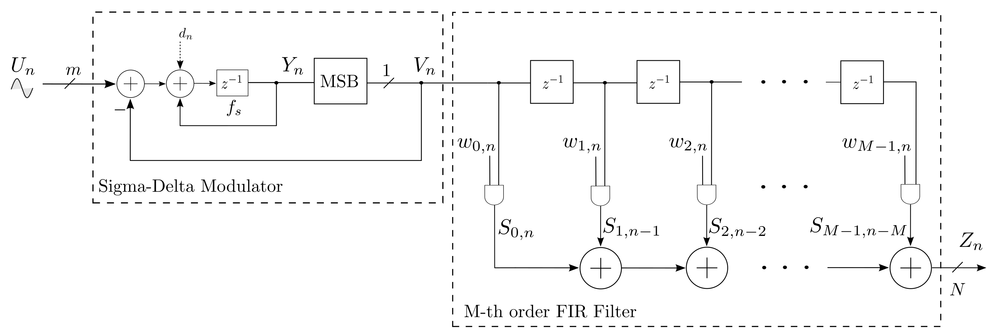
4. Proposed SDM-SC Processing Scheme

In this section, we present the proposed SDM-SC architecture as it was introduced in [26], and is shown in Figure 6. It converts a multi-bit input signal into a single-bit one using a first-order SDM to exploit the SC’s encoding and benefit from its low-area advantages. Moreover, it allows for time-encoding and, consequently, processing of the input signal, therefore bypassing the long-latency of the standard SC approaches. To proceed with the detailed analysis of the architecture, we start from the first-order SDM.

4.1. SDM Encoding

In the architecture of Figure 6, the SDM block is the digital realization of the system-level one shown in Figure 3. Its input $U_n$ is of m-bits length, whereas $V_n$ is the single-bit output. A register of c-bits can replace the integrator of Figure 3, allowing for the SDM’s iterative behavior to be expressed according to Equation (14). With respect to its size (in bits), it should be noted that $c\ge m$ so as to account for the accumulation process, with typical value $c=m+1$.

The quantization process of the SDM in Figure 3 can be modeled simply as the register’s most significant bit (MSB); the current input sample, i.e., $U_n$, determines if, and only if, the accumulator’s current value is positive or negative, corresponding to an MSB of 0 or 1, respectively. Finally, it should be noted that $V_n$’s negative value, i.e., 1, is converted into $-1$ using sign-extension methods.

The SDM’s maximum operating frequency $f_s$ corresponds to the register’s one and, as expected, determines the input signal’s maximum operating frequency $f_B$ that the architecture is able to process. Optionally, a dithering sequence can be employed to further decrease the SDM’s output noise floor [32,33,34].

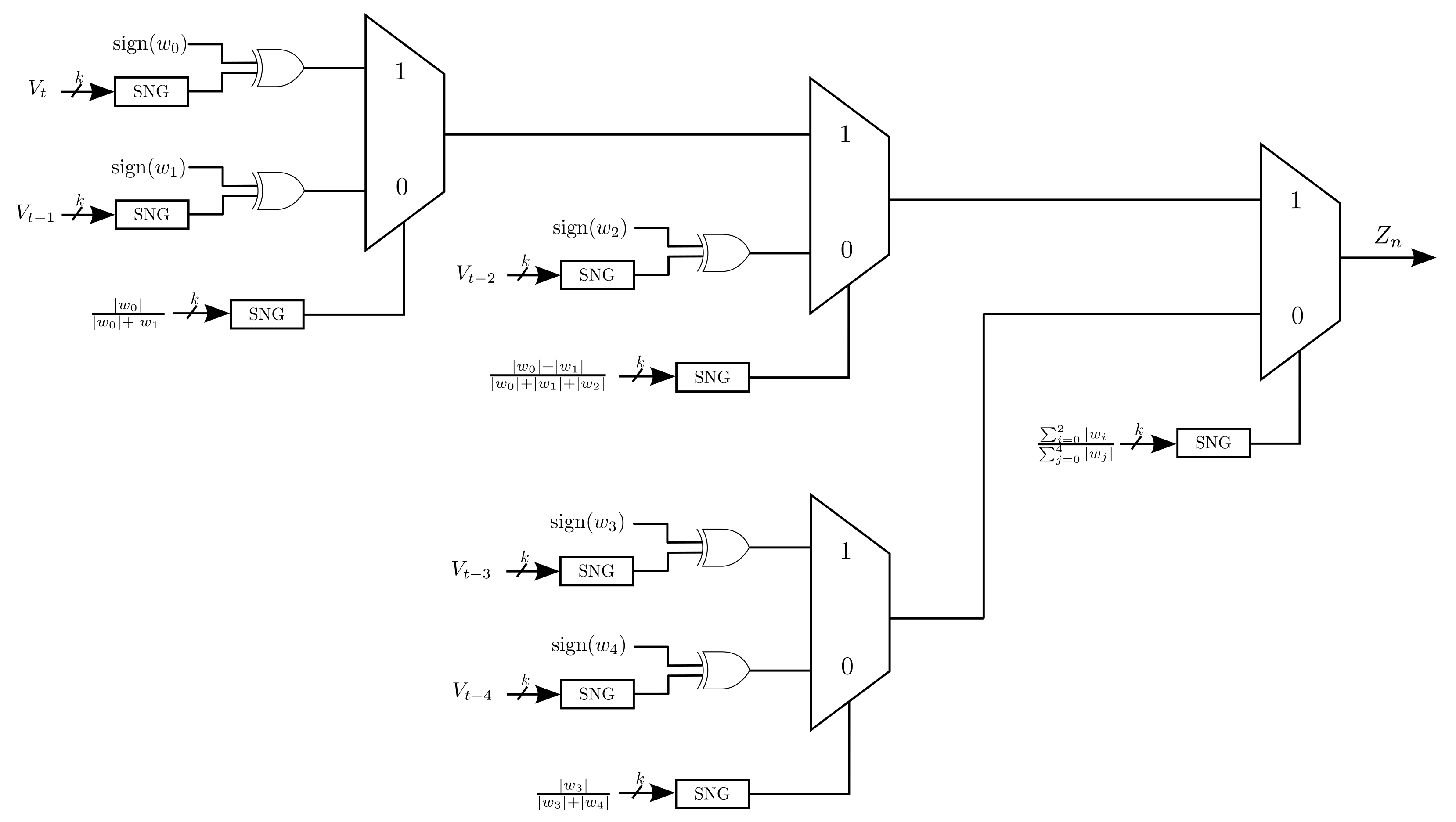
4.2. Stochastic FIR Filter

According to Equation (15), the binary implementation of an M-tap FIR filter requires $M-1$ D flip-flops, M binary multipliers of $m+l$-bit length, where m and l are the input signal’s and the coefficient’s bit resolutions, respectively, and a binary adder of $m+l+lo{g}_2\left(M\right)-1$ bits to avoid overflows, based on the guidelines in [42].

The architecture of Figure 6 exploits the SDM’s $0,1$ encoding of the input signal, allowing for the M binary multipliers of $m+l$-bit length to be replaced by M AND gates. Furthermore, in contrast to the standard adder method used in SC, which is based upon the realization of an adder tree using the inner-product processing block of Figure 4, we use a simple binary adder of $N=\lceil lo{g}_{2}M\rceil$-bits. As such, the value of $Z_n$ is binary and belongs in $\{0,1,\cdots ,M-1\}$. At this point, we note that one can also explore single-bit output implementations of the proposed architecture, using several non-scaling adders available in the SC literature [11,20,43].

To proceed with further analysis, we assume that each weight is converted into a stochastic sequence with probability $w_m=P(w_{m,n}=1)$, with $m=1,2,\cdots ,M$, and also that the probability of each AND gate’s output is

$$\begin{array}{c}\hfill S_m=P(S_{m,n}=1)=P(w_{m,n}=1)V_n.\end{array}$$

(19)

Considering the above and the architecture of Figure 6, the instantaneous value of the output $Z_n$ is the sum of the multiplications and is given as

$$\begin{array}{c}\hfill Z_n=\sum _{m=0}^{M-1}{S}_m.\end{array}$$

(20)

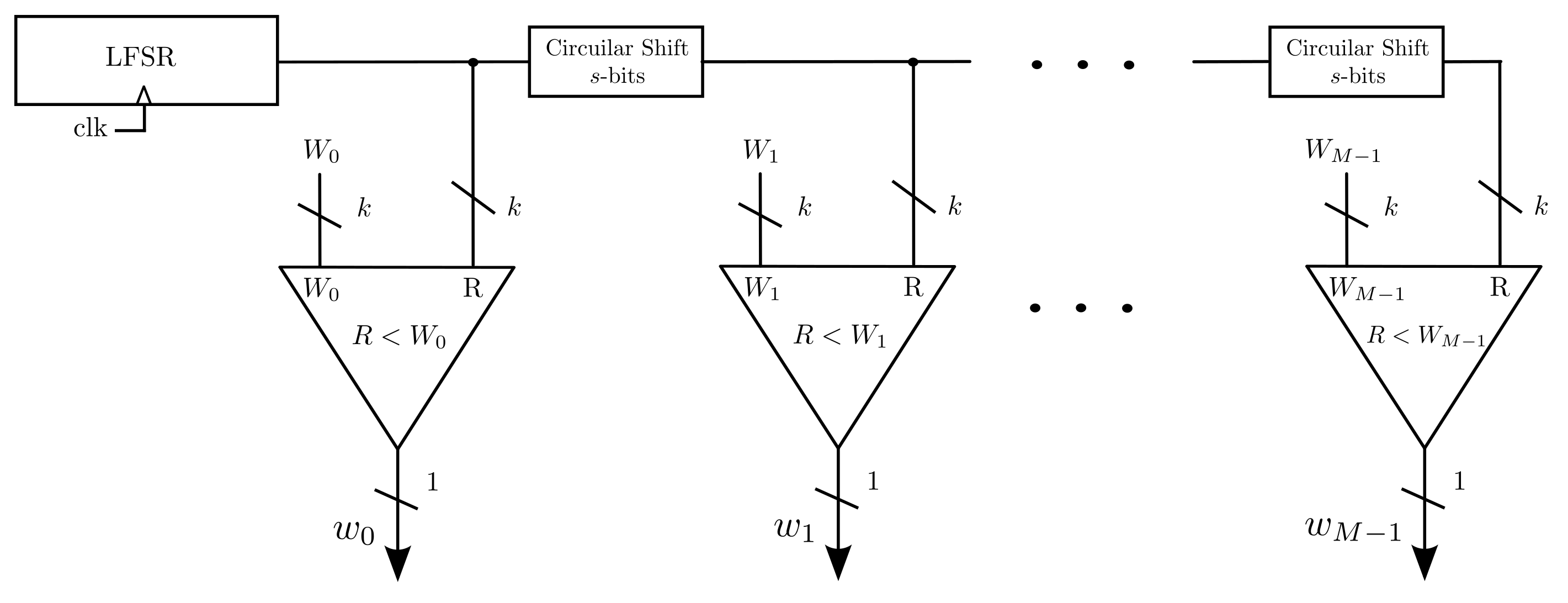
4.3. Stochastic Coefficient Generation

The conversion of the filter’s coefficients $w_m$ to stochastic numbers in the architecture of Figure 6 requires M SNGs. This, however, implies the use of M LFSRs of k-bits, which, along with their respective k-bit comparators, are hardware-taxing (in total, $k\times M$ registers). On the other hand, simple sharing of a single LFSR, as the random number generator between all SNGs, introduces maximal correlation among the generated sequences according to Equation (Section 2.3), and thus it is expected to degrade the filtered signal’s spectral quality [26,41].

In order to reduce the hardware resources from the SNGs, we employ the LFSR circular shifting scheme proposed in [44], shown in Figure 7. This scheme generates M stochastic sequences in parallel without being maximally correlated using a single LFSR. This is achieved, since the LFSR cycles through all of its values within ${\mathcal{R}}_s$ only once. Therefore, if $R_{n,i}$ is the LFSR’s current binary value n at time index $i=1,2,\cdots ,M$, the circular shift by $s\in {\mathbb{N}}^{*}$ bits, where $s<k$, produces the next value $R_{n,i+1}$ as

$$R_{n,i+1}\triangleq R_{{(n-s,i)}_N}=R_{n-s,i}modN.$$

(21)

5. Experimental Results

In this section, we demonstrate the performance of the proposed SDM-SC architecture. Specifically, we show experimental results with respect to 1) its spectral characteristics, and 2) comparisons with standard SC-based approaches, as well as with the conventional binary, in SNR and hardware resources.

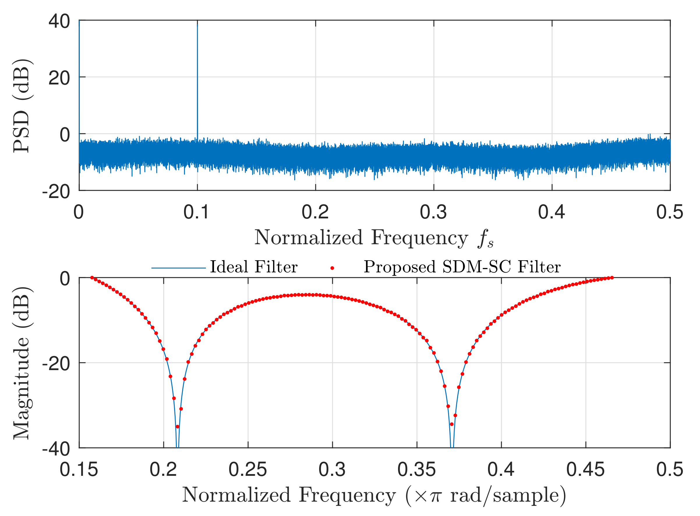
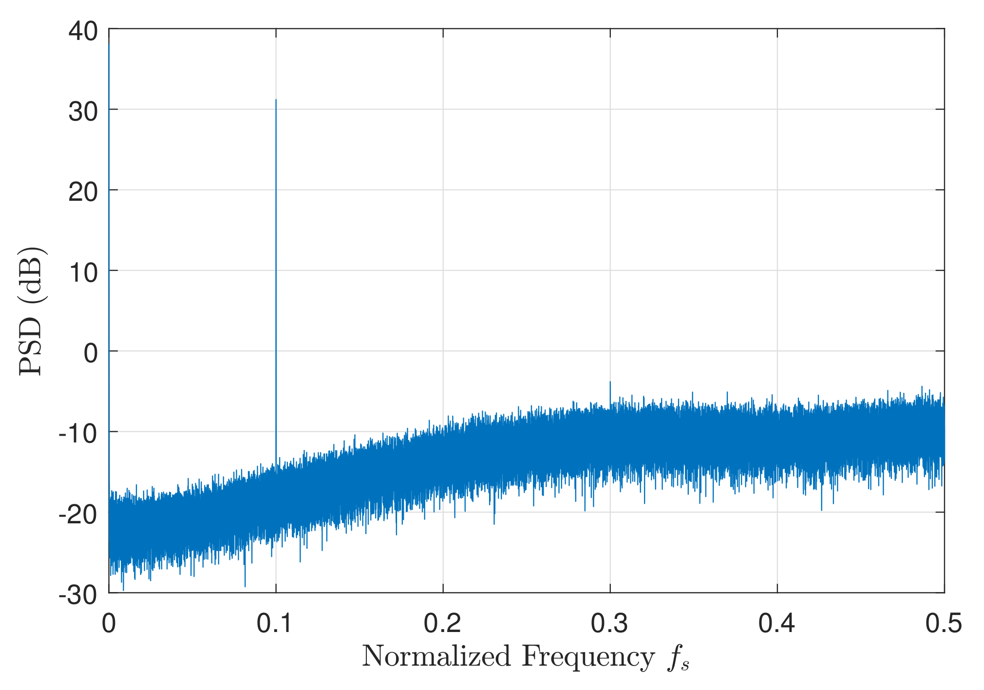
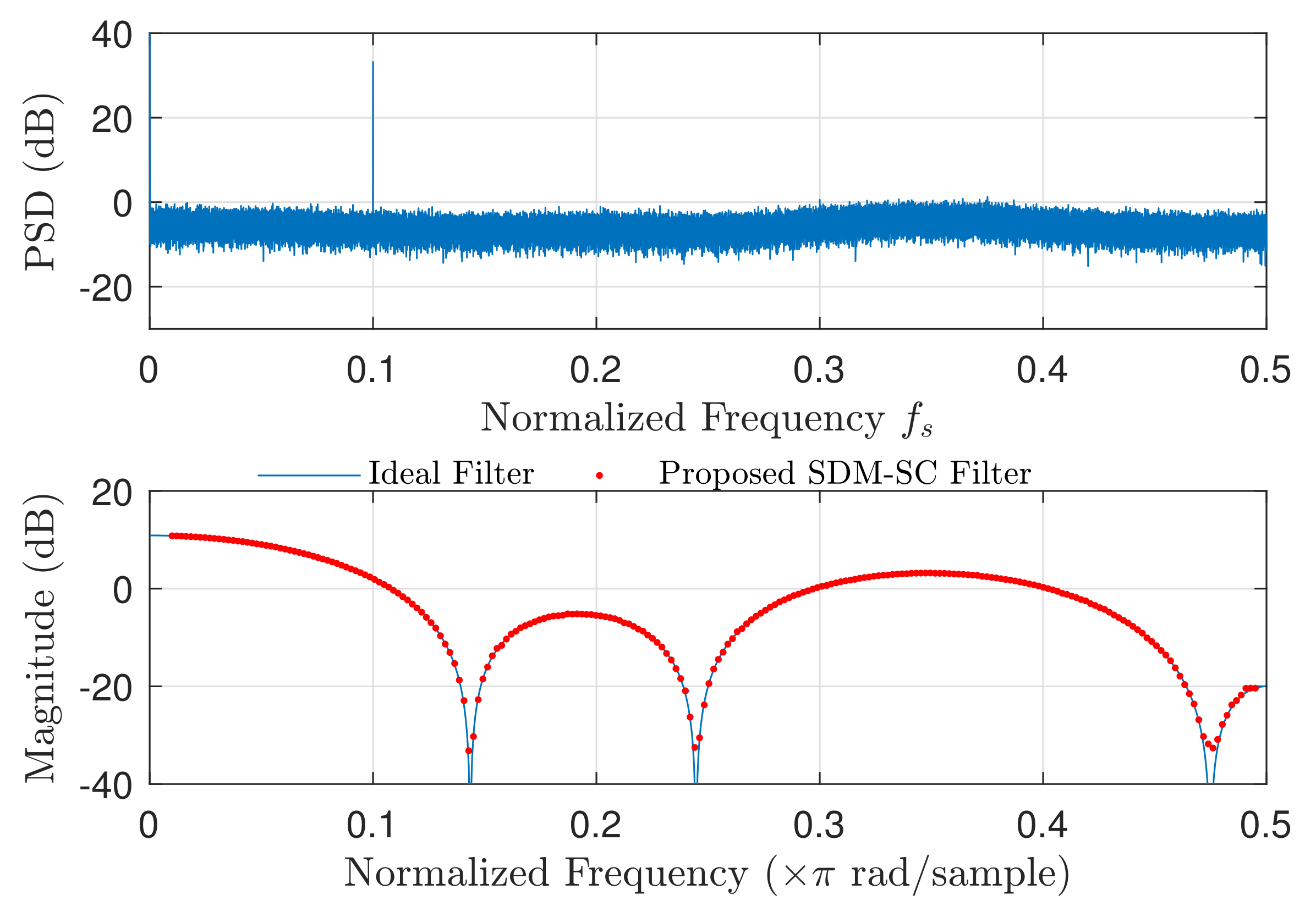
5.1. Performance of the Proposed SDM-SC Architecture in the Spectral Domain

Here, we evaluate the performance of the proposed SDM-SC architecture in the spectral domain with simulations using MATLAB. We consider a sinusoidal input signal $U_n=sin\left(2\pi f_{B}n\right)$, and test it over two FIR filters, a 5- and a 7-tap one. The simulation parameters, including the filters’ weights, are summarized in

Table 1. Simulation parameters.

Parameter Name	Parameter Value
Input signal $U_n$	$sin\left(2\pi f_{B}n\right)$
5-tap FIR filter weights	$w_0=w_4=0.7,w_1=w_3=0.6,w_2=0.9$
7-tap FIR filter weights	$w_0=w_6=0.6,w_1=w_5=0.4,w_2=w_4=0.3,w_3=0.9$

.

It is important to note that all frequencies are fractional with respect to the sampling frequency $f_s$. Moreover, to generate the sequences of the weights, LFSRs with initial register size of 15-bits are used and correspond to sequences with length $2^{15}$.

In Figure 8 and Figure 9, the power spectral density (PSD) (top) and frequency response (bottom) for the 5 and 7-tap FIR filters are respectively shown. To calculate the power spectral density, MATLAB’s pwelch function was used and ${10}^6$ samples were considered. With respect to the frequency response, it can be observed that the SDM-SC architecture follows the conventional one’s, correctly achieving the cut-off frequency ${\omega }_{-3\mathrm{dB}}$.

To showcase the ability of the proposed SDM-SC architecture to achieve improved performance, we show the power spectral density of the SDM’s output in Figure 10. It is calculated using MATLAB’s pwelch function with ${10}^6$ samples. As one can observe the SDM reduces the noise floor in low frequencies.

5.2. Signal-to-Noise Ratio Comparisons

Here, we show the advantage of the proposed SDM-SC architecture over the standard SC-based implementations with SNR comparisons. We realize the 5- and 7-tap FIR filters using the inner-product module of Figure 4, with their coefficient values taken from Table 1 With respect to the conventional binary approach, we assumed the existence of round-off noise in the coefficients and in the input signal, where the bit resolution is selected to be 15-bits. In

Table 2. SNR Comparison for the 5 & 7-tap FIR filters.

	5-Tap FIR Filter			7-Tap FIR Filter
	SDM-SC	Inner-Product Adder-Tree [29,30,41]	Conv. Binary	SDM-SC	Inner-Product Adder-Tree [29,30,41]	Conv. Binary
SNR (dB)	47.01	31.41	97.21	42.94	29.93	91.31

, the SNR comparison between the two approaches is shown, accompanied by the conventional binary.

According to the results shown in Table 2, the proposed SDM-SC filtering scheme achieves better SNR than the filtering realized using the inner-product module of Figure 4, which is due to the SDM’s oversampling. On the other hand, compared to the traditional binary, the SDM-SC architecture achieves lower SNR. Yet, its negligible low-area advantages as an approximate filtering scheme are highlighted in the following subsection.

5.3. FPGA Synthesis Results and Comparison

The low-area benefits of the proposed SDM-SC architecture are demonstrated here. We compared its hardware resources required to realize the two FIR filters with 5 and 7 taps, with the conventional binary and the inner-product approach synthesized in Xilinx’s Vivado Design Suite targeting the Kintex-7 FPGA KC705 device. We considered a $k=15$-bit resolution of the input signal U, which also corresponds to the LFSR’s size used to generate the weights, $w_m$. The hardware utilization results are cited in

Table 3. Comparison of FPGA synthesis results for two FIR filters with 5 & 7 taps.

	5-Tap FIR Filter
	SDM-SC Filter	Inner-Product Adder-Tree [29,30,41]	Conv. Binary
Max Operating Frequency (MHz)	667
Slice LUTs [Used/Util.]	29/0.01%	35/0.01%	698/0.34%
Slice Registers [Used/Util.]	35/0.01%	178/0.05%	60/0.02%
	7-tap FIR filter
	SDM-SC Filter	Inner-Product Adder-Tree [29,30,41]	Conv. Binary
Max Operating Frequency (MHz)	667
Slice LUTs [Used/Util.]	30/0.01%	42/0.01%	907/0.45%
Slice Registers [Used/Util.]	37/0.01%	238/0.06%	90/0.02%

. For the results shown, we note the following: (1) for the conventional binary approach, the DSP blocks are converted into their LUT equivalents to have a uniform comparison of the resources among the approaches considered, and (2) the SNGs are included in the utilization results.

According to the results shown in Table 3, the proposed SDM-SC architecture can realize a 5-tap FIR filter with 29 LUTs and 35 registers. On the contrary, the inner-product FIR approach based on [29,30,41] requires only a few LUTs more, namely 35, but also 143 register slices more, which is due to the required SNGs for (1) the MUXs and (2) the generation of the input signal’s delays. The conventional binary five-tap FIR filter requires additionally 669 LUTs and 25 slice registers (in total, 698 LUTs and 60 slice registers), making the SDM-SC architecture a hardware-favored approach as it reduces the LUTs by $96\%$ and the slice registers by $42\%$ of the binary filter.

To realize the 7-tap filter, the SDM-SC architecture requires only two registers and one LUT more; increasing the order of the filter by two requires two delays, corresponding to two flip-flops as a result of the SDM’s single bit encoding, while the one LUT increase is due to the additional wiring required to output the result. The inner-product approach, however, requires 60 slice registers more to increase the filter’s order by two, which is due to the four SNGs required for the addition of an inner-product block as well as the MUX producing the output. The increase on the hardware resources is also observed when the conventional binary FIR filter’s order is increased, which is equal to 209 LUT and 30 register slices more. As such, the SDM-SC architecture reduces, in this case, the binary realization’s LUT and slice register utilization by $96.7\%$ and $60\%$, respectively.

5.4. Hardware Resources Comparison in a 45 nm Technology

To further proceed with the hardware comparisons, here we provide the resources required to realize the two FIR filters with 5 and 7 taps, extracted using the Synopsys Design Compiler with the FreePDK CMOS library at 45 nm [45]. For the comparisons, the following estimates are provided: (1) the total area in $\left(\mathsf{\mu }{\mathrm{m}}^2\right)$; (2) the average power consumption in mW; (3) the delay in ns; (4) the energy consumption in pJ, defined as the average power × delay product. In

Table 4. Comparison of hardware resources for the realization of two FIR filters with 5 & 7 taps in area $\left(\mathsf{\mu }{\mathrm{m}}^2\right)$, power (mW), delay (ns), and energy (pJ).

	5-Tap FIR Filter
	SDM-SC Filter	Inner-Product Adder-Tree [29,30,41]	Conv. Binary
Area $\left(\mathsf{\mu }{\mathrm{m}}^2\right)$	617.12	3425.88	9853.89
Power (mW)	0.75	2.97	5.19
Delay (ns)	$1.5$
Energy (pJ)	1.13	4.46	7.78
	7-tap FIR filter
	SDM-SC Filter	Inner-Product Adder-Tree [29,30,41]	Conv. Binary
Area $\left(\mathsf{\mu }{\mathrm{m}}^2\right)$	700.66	4935.67	13,428.55
Power (mW)	0.83	4.39	7.12
Delay (ns)	$1.5$
Energy (pJ)	1.24	6.51	10.58

, the results are shown in detail.

Focusing on the realization of the 5-tap FIR filter, when compared to the inner-product and conventional binary approaches, the proposed SDM-SC architecture reduces, respectively, 1) the total area occupied by $81.9\%$ and $93.7\%$, and 2) the total power and energy consumption by $74.7\%$ and $85.5\%$. For the realization of the 7-tap FIR filter, the proposed SDM-SC architecture reduces, respectively, 1) the total area occupied by $85.8\%$ and $94.8\%$, and 2) the total power and energy consumption by $81.09\%$ and $88.34\%$. As such, from Table 4, one can conclude that the proposed SDM-SC architecture is the most efficient, hardware-wise, as it results in the least occupied area and power and energy consumption among the considered approaches.

Of great interest is the number of resources required to increase the filter’s order. The SDM-SC architecture requires only 83.54 $\mathsf{\mu }{\mathrm{m}}^2$, $0.08$ mW, and $0.11$ pJ, corresponding to an increase of the resources by $11.9\%$, $9.6\%$, and $8.8\%$, respectively. On the other hand, the inner-product approach requires 1509.8 $\mathsf{\mu }{\mathrm{m}}^2$, $1.42$ mW, and 2.05 pJ, corresponding to an increase of the resources by $30.5\%$, $32.3\%$, and $31.4\%$, respectively, whereas the conventional binary requires 3574.7 $\mathsf{\mu }{\mathrm{m}}^2$, 1.93 mW, and 2.8 pJ, corresponding to an increase of the resources by $26.6\%$, $27.1\%$, and $26.4\%$, respectively.

A further advantage of the SDM-SC’s architecture in filtering over the inner-product approach is that of time-encoding. Assuming that the input signal $U_n$ is of length $\widehat{N}$, then the SDM-SC approach processes $\widehat{N}$ samples in N clock cycles, whereas the inner-product approach requires N clock cycles for a single sample of $\widehat{N}$, thus requiring $N\times \widehat{N}$ clock cycles to complete the processing. This, however, reflects on the total dissipated energy by the inner-product approach, which is increased by N. Therefore, this makes the SDM-SC architecture both faster in terms of processing time and a more energy-efficient approximate processing approach, besides its improved SNR performance.

6. Conclusions

A soft-filtering architecture based on SDMs and SC was presented in this work. The first-order SDM acts as a single-bit encoder to benefit from the negligible area SC multipliers, implemented as XNOR gates. The performance of the SDM-SC architecture was evaluated in two different-order FIR filters in the spectral domain, where the filters’ proper operation and roll-off behavior were shown. Compared to the standard SC-based filtering approach, it was shown that the SDM-SC architecture improves the SNR by more than 10 dB, while at the same time eliminates the SC’s typical latency–accuracy trade-off, as it provides encoding in time, reflecting on the power and energy consumption, as well. With respect to the hardware resources, FPGA and synopsys synthesis results demonstrated the SDM-SC’s negligible area advantages and its highly energy-efficient processing over standard SC-based and binary approaches.

References

1. Mounica, Y.; Kumar, K.N.; Veeramachaneni, S.; Mahammad, N. Energy efficient signed and unsigned radix 16 booth multiplier design. Comput. Electr. Eng. 2021, 90, 106892. [Google Scholar] [CrossRef]
2. Leon, V.; Paparouni, T.; Petrongonas, E.; Soudris, D.; Pekmestzi, K. Improving Power of DSP and CNN Hardware Accelerators Using Approximate Floating-point Multipliers. ACM Trans. Embed. Comput. Syst. 2021, 20, 1–21. [Google Scholar] [CrossRef]
3. Alaghi, A.; Qian, W.; Hayes, J.P. The Promise and Challenge of Stochastic Computing. IEEE Trans. Comput.-Aided Des. Integr. Circuits Syst. 2018, 37, 1515–1531. [Google Scholar] [CrossRef]
4. Gross, W.J.; Gaudet, V.C. Stochastic Computing: Techniques and Applications; Springer, International Publishing, Springer Nature Switzerland AG: Cham, Switzerland, 2019. [Google Scholar]
5. Alaghi, A.; Hayes, J.P. Survey of Stochastic Computing. ACM Trans. Embed. Comput. Syst. 2013, 12, 1–19. [Google Scholar] [CrossRef]
6. Metku, P.; Seva, R.; Choi, M. Energy-Performance Scalability Analysis of a Novel Quasi-Stochastic Computing Approach. MDPI J. Low Power Electron. Appl. 2019, 9, 30. [Google Scholar] [CrossRef] [Green Version]
7. Gaines, B.R. Stochastic Computing Systems; Springer: Boston, MA, USA, 1967. [Google Scholar]
8. Najafi, M.H.; Jenson, D.; Lilja, D.J.; Riedel, M.D. Performing Stochastic Computation Deterministically. IEEE Trans. Very Large Scale Integr. (VLSI) Syst. 2019, 27, 2925–2938. [Google Scholar] [CrossRef]
9. Temenos, N.; Sotiriadis, P.P. Deterministic Finite State Machines for Stochastic Division in Unipolar Format. In Proceedings of the IEEE International Symposium on Circuits and Systems (ISCAS), Seville, Spain, 12–14 October 2020. [Google Scholar]
10. Lee, V.T.; Alaghi, A.; Hayes, J.P.; Sathe, V.; Ceze, L. Energy-efficient hybrid stochastic-binary neural networks for near-sensor computing. In ACM Proceedings of the Conference on Design, Automation & Test in Europe, Laussane, Switzerland, 27–31 March 2017. [Google Scholar]
11. Yuan, B.; Wang, Y.; Wang, Z. Area-Efficient Scaling-Free DFT/FFT Design Using Stochastic Computing. IEEE Trans. Circuits Syst. II Express Briefs 2016, 63, 1131–1135. [Google Scholar] [CrossRef]
12. Ting, P.; Hayes, J.P. Eliminating a hidden error source in stochastic circuits. In Proceedings of the IEEE International Symposium on Defect and Fault Tolerance in VLSI and Nanotechnology Systems (DFT), Cambridge, UK, 23–25 October 2017. [Google Scholar]
13. Morro, A.; Canals, V.; Oliver, A.; Alomar, M.L.; Galán-Prado, F.; Ballester, P.J.; Rosselló, J.L. A Stochastic Spiking Neural Network for Virtual Screening. IEEE Trans. Neural Netw. Learn. Syst. 2018, 29, 1371–1375. [Google Scholar] [CrossRef] [PubMed]
14. Brown, B.D.; Card, H.C. Stochastic Neural Computation I: Computational Elements. IEEE Trans. Comput. 2002, 50, 891–905. [Google Scholar] [CrossRef]
15. Brown, B.D.; Card, H.C. Stochastic Neural Computation II: Soft Competitive Learning. IEEE Trans. Comput. 2002, 50, 906–920. [Google Scholar] [CrossRef]
16. Ardakani, A.; Leduc-Primeau, F.; Onizawa, N.; Hanyu, T.; Gross, W.J. VLSI Implementation of Deep Neural Network Using Integral Stochastic Computing. IEEE Trans. Very Large Scale Integr. (VLSI) Syst. 2017, 25, 2688–2699. [Google Scholar] [CrossRef] [Green Version]
17. Liu, S.; Jiang, H.; Liu, L.; Han, J. Gradient Descent Using Stochastic Circuits for Efficient Training of Learning Machines. IEEE Trans. Comput.-Aided Des. Integr. Circuits Syst. 2018, 37, 2530–2541. [Google Scholar] [CrossRef]
18. Liu, Y.; Liu, L.; Lombardi, F.; Han, J. An Energy-Efficient and Noise-Tolerant Recurrent Neural Network Using Stochastic Computing. IEEE Trans. Very Large Scale Integr. (VLSI) Syst. 2019, 27, 2213–2221. [Google Scholar] [CrossRef]
19. Liu, Y.; Liu, S.; Wang, Y.; Lombardi, F.; Han, J. A Survey of Stochastic Computing Neural Networks for Machine Learning Applications. IEEE Trans. Neural Netw. Learn. Syst. 2020, 32, 2809–2824. [Google Scholar] [CrossRef]
20. Temenos, N.; Sotiriadis, P.P. Nonscaling Adders and Subtracters for Stochastic Computing Using Markov Chains. IEEE Trans. Very Large Scale Integr. Syst. (VLSI) 2021, 29, 1612–1623. [Google Scholar] [CrossRef]
21. Li, P.; Lilja, D.J. Using Stochastic Computing to Implement Digital Image Processing Algorithms. In Proceedings of the IEEE 29th International Conference on Computer Design (ICCD), Amherst, MA, USA, 9–12 October 2011. [Google Scholar]
22. Li, P.; Lilja, D.J.; Qian, W.; Bazargan, K.; Riedel, M.D. Computation on Stochastic Bit Streams Digital Image Processing Case Studies. IEEE Trans. Very Large Scale Integr. Syst. (VLSI) 2014, 2, 449–462. [Google Scholar] [CrossRef]
23. Alaghi, A.; Li, C.; Hayes, J.P. Stochastic circuits for real-time image-processing applications. In Proceedings of the IEEE 50th ACM/EDAC/IEEE Design Automation Conference (DAC), Austin, TX, USA, 29 May–7 June 2013. [Google Scholar]
24. Temenos, N.; Sotiriadis, P.P. Stochastic Computing Max & Min Architectures Using Markov Chains: Design, Analysis, and Implementation. IEEE Trans. Very Large Scale Integr. Syst. (VLSI) 2021, 29, 1813–1823. [Google Scholar]
25. Alawad, M.; Lin, M. Fir filter based on stochastic computing with reconfigurable digital fabric. In Proceedings of the IEEE 23rd Annual International Symposium on Field-Programmable Custom Computing Machines, Vancouver, BC, Canada, 2–6 May 2015. [Google Scholar]
26. Vlachos, A.; Temenos, N.; Sotiriadis, P.P. Exploring the Effectiveness of Sigma-Delta Modulators in Stochastic Computing-Based FIR Filtering. In Proceedings of the IEEE 10th International Conference on Modern Circuits and Systems Technologies (MOCAST), Thessaloniki, Greece, 5–7 July 2021. [Google Scholar]
27. Saraf, N.; Bazargan, K.; Lilja, D.J.; Riedel, M.D. IIR filters using stochastic arithmetic. In Proceedings of the IEEE Design, Automation & Test in Europe Conference & Exhibition (DATE), Dresden, Germany, 24–28 March 2014. [Google Scholar]
28. Ahmed, K.J.; Yuan, B.; Lee, M.J. High-Accuracy Stochastic Computing-Based FIR Filter Design. In Proceedings of the IEEE International Conference on Acoustics, Speech and Signal Processing (ICASSP), Calgary, AB, Canada, 15–20 April 2018. [Google Scholar]
29. Ichihara, H.; Sugino, T.; Ishii, S.; Iwagaki, T.; Inoue, T. Compact and Accurate Digital Filters Based on Stochastic Computing. IEEE Trans. Emerg. Top. Comput. 2019, 7, 31–43. [Google Scholar] [CrossRef]
30. Liu, Y.; Parhi, K.K. Architectures for Recursive Digital Filters Using Stochastic Computing. IEEE Trans. Signal Process. 2016, 64, 3705–3718. [Google Scholar] [CrossRef]
31. Tehrani, S.S.; Gross, W.J.; Mannor, S. Stochastic decoding of LDPC codes. IEEE Commun. Lett. 2006, 10, 716–718. [Google Scholar] [CrossRef]
32. Basetas, C.; Temenos, N.; Sotiriadis, P.P. Comparison of Recently Developed Single-Bit All-Digital Frequency Synthesizers in Terms of Hardware Complexity and Performance. In Proceedings of the IEEE International Symposium on Circuits and Systems (ISCAS), Florence, Italy, 27–30 May 2018. [Google Scholar]
33. Basetas, C.; Temenos, N.; Sotiriadis, P.P. An Efficient Hardware Architecture for the Implementation of Multi-Step Look-Ahead Sigma-Delta Modulators. In Proceedings of the IEEE International Symposium on Circuits and Systems (ISCAS), Florence, Italy, 27–30 May 2018. [Google Scholar]
34. Schreier, R.; Temes, G.C. Understanding Delta-Sigma Data Converters; John Wiley & Sons, Inc.: Hoboken, NJ, USA, 2005. [Google Scholar]
35. Liu, S.; Han, J. Toward Energy-Efficient Stochastic Circuits Using Parallel Sobol Sequences. IEEE Trans. Very Large Scale Integr. (VLSI) Syst. 2018, 26, 1326–1339. [Google Scholar] [CrossRef]
36. Qian, W.; Li, X.; Riedel, M.D.; Bazargan, K.; Lilja, D. An Architecture for Fault-Tolerant Computation with Stochastic Logic. IEEE Trans. Comput. 2011, 60, 93–105. [Google Scholar] [CrossRef]
37. Camps, O.; Stavrinides, S.; Picos, R. Stochastic Computing Implementation of Chaotic Systems. Mathematics 2021, 9, 375. [Google Scholar] [CrossRef]
38. Lee, V.T.; Alaghi, A.; Ceze, L. Correlation manipulating circuits for stochastic computing. In Proceedings of the IEEE Design, Automation & Test in Europe Conference & Exhibition (DATE), Dresden, Germany, 19–23 March 2018. [Google Scholar]
39. Alaghi, A.; Hayes, J.P. Exploiting correlation in stochastic circuit design. In Proceedings of the IEEE 31st International Conference on Computer Design (ICCD), Asheville, NC, USA, 6–9 October 2013. [Google Scholar]
40. Liu, Y.; Parhi, M.; Riedel, M.D.; Parhi, K.K. Synthesis of Correlated Bit Streams for Stochastic Computing. In Proceedings of the IEEE 50th Asilomar Conference on Signals, Systems and Computers, Pacific Grove, CA, USA, 6–9 November 2016. [Google Scholar]
41. Chang, Y.; Parhi, K.K. Architectures for digital filters using stochastic computing. In Proceedings of the IEEE International Conference on Acoustics, Speech and Signal Processing, Vancouver, BC, Canada, 26–31 May 2013. [Google Scholar]
42. Meyer-Baese, U. Digital Signal Processing with Field Programmable Gate Arrays, 4th ed.; Springer: Berlin/Heidelberg, Germany, 2014. [Google Scholar]
43. Ren, A.; Li, Z.; Ding, C.; Qiu, Q.; Wang, Y.; Li, K.; Qian, X.; Yuan, B. SC-DCNN: Highly-Scalable Deep Convolutional Neural Network using Stochastic Computing. In Proceedings of the ACM 22nd International Conference on Architectural Support for Programming Languages and Operating Systems(ASPLOS), Xi’an, China, 8–12 April 2017. [Google Scholar]
44. Ichihara, H.; Ishii, S.; Sunamori, D.; Iwagaki, T.; Inoue, T. Compact and Accurate Stochastic Circuits with Shared Random Number Sources. In Proceedings of the IEEE 32nd International Conference on Computer Design (ICCD), Seoul, Korea, 19–22 October 2014. [Google Scholar]
45. Stine, J.E.; Castellanos, I.; Wood, M.; Henson, J.; Love, F.; Davis, W.R.; Franzon, P.D.; Bucher, M.; Basavarajaiah, S.; Oh, J.; et al. FreePDK: An Open-Source Variation-Aware Design Kit. In Proceedings of the IEEE International Conference on Microelectronic Systems Education, San Diego, CA, USA, 3–4 June 2007. [Google Scholar]
Figure 1. Stochastic sequence generation: (a) Stochastic number generator (SNG) block; (b) Equivalent block.
Technologies 10 00014 g001
Figure 2. Stochastic computing fundamental operations: (a) Unipolar multiplication, (b) bipolar multiplication, (c) unipolar/bipolar addition.
Technologies 10 00014 g002
Figure 3. The first-order single-bit sigma-delta modulator. A dithering sequence can optionally be used.
Technologies 10 00014 g003
Figure 4. Inner-product block with two inputs.
Technologies 10 00014 g004
Figure 5. Stochastic implementation of a five-tap FIR filter based on the inner-product block of Figure 4.
Technologies 10 00014 g005
Figure 6. Proposed SDM-SC architecture. The first-order SDM encodes a multi-bit input signal into a single-bit one, carrying the information in 0 , 1 representation. The sequence is then processed by an SC-based M-tap FIR filter. A dithering sequence can optionally be used.
Technologies 10 00014 g006
Figure 7. SNG sharing scheme with circular shifting.
Technologies 10 00014 g007
Figure 8. Power Spectral Density (top) using pwelch with 10 6 samples and frequency response (bottom) of the SDM-SC architecture for a 5-tap FIR filter. Weights’ values are cited in Table 1.
Technologies 10 00014 g008
Figure 9. Power Spectral Density (top) using pwelch with 10 6 samples and frequency response (bottom) of the SDM-SC architecture for a 7-tap FIR filter. Weights’ values are cited in Table 1.
Technologies 10 00014 g009
Figure 10. Power Spectral Density of the SDM’s output calculated using pwelch with 10 6 samples.
Technologies 10 00014 g010