Chaotic Scaling and Network Turbulence in Crude Oil-Equity Systems Using a Coupled Multiscale Chaos Index

Abstract

Financial markets often display nonlinear and turbulent dynamics during periods of stress, and crude-oil and global equity systems frequently demonstrate closely connected forms of instability. Earlier studies report multifractality, chaotic features and regime-dependent spillovers across commodities and equities, yet existing approaches rarely succeed in capturing both the intrinsic complexity of oil-market behavior and the changing structure of cross-asset dependence. This limitation reduces the ability to distinguish calm from turbulent regimes and weakens short-horizon risk assessment. The present study introduces a unified framework that quantifies and predicts systemic instability within the coupled oil–equity system. The analysis constructs a crude-oil complexity index based on multifractal fluctuation analysis, permutation and approximate entropy, and Lyapunov-based indicators of chaotic dynamics. At the same time, it develops an information-theoretic network of global equity and energy-sector returns and summarizes its instability through measures of edge turnover, spectral radius, degree entropy and strength dispersion. These components are combined to form the Coupled Multiscale Chaos Index (CMCI), a scalar state variable that distinguishes calm, transitional and chaotic market regimes. Empirical results indicate that Brent and WTI exhibit pronounced multifractality, elevated entropy and positive Lyapunov exponents, while the dependence network becomes more centralized, more clustered and more capable of shock amplification during high-CMCI states. The CMCI moves closely with realized volatility and provides significant predictive content for five-day variance across major global equity benchmarks, with performance superior to models that rely only on macro-financial controls. Out-of-sample evaluation shows that forecasts incorporating measures of complexity record substantially lower MSE and QLIKE losses. The findings indicate that systemic instability reflects the interaction between local chaotic dynamics in crude-oil markets and turbulence in the global dependence network. The CMCI offers a practical early-warning indicator that supports risk management, forecasting and macroprudential supervision.

1. Introduction

1.1. Motivation

Modern financial systems are inherently complex, characterized by nonlinear interactions across markets that can amplify shocks and blur the line between real economic forces and speculative dynamics. This complexity becomes especially clear when examining major disruptions in energy. Episodes such as the 2014–2016 oil-price collapse, the COVID-19 shock, and the subsequent monetary tightening cycle have shown that disturbances originating in oil markets can spill over rapidly into global equity and sector indices (Sadraoui & Sallam, 2025). These episodes are frequently characterized as multifractal, chaotic, or turbulent terms that underscore the presence of irregular yet systematically patterned price dynamics and abrupt shifts in cross-asset dependencies (Kristjanpoller, 2025). Accurately distinguishing periods of relative stability from those of heightened disorder within the coupled oil–equity system and understanding how these regimes map onto short-horizon risk are thus of critical importance for investors, risk managers, and policymakers.

Crude oil and equity markets exhibit several features that complicate standard risk modeling. At the time-series level, returns display scale-dependent irregularities, long-memory dynamics, and behaviors often associated with complex or chaotic systems (A. O. Bielinskyi & Serdyuk, 2021). At the cross-sectional level, shocks propagate through a fluid network of dependencies linking broad equity indices, sectoral portfolios, and energy-related assets. These networks can restructure rapidly, with shifts in connectivity, clustering, and the relative importance of different assets that are not well captured by simple linear relationships (Ahmed et al., 2024). Consequently, risk emerges through mechanisms that act both within localized temporal fluctuations and across broader system-wide interdependencies. Despite this, comparatively little is known about how the multifractal and potentially chaotic features of crude oil markets interact with the evolving network structure that connects energy and equity assets, or whether this interaction can be distilled into a parsimonious state variable that is economically interpretable and empirically informative for distinguishing calm from chaotic regimes and for modeling short-horizon variance and drawdown risk (Fischer, 2023).

To address this gap, this study advances a new framework designed to capture the joint dynamics of oil-market complexity and the evolving structure of energy–equity linkages. The approach unfolds in three stages, described in Section 2. First, we construct an index that reflects the degree of instability and irregularity in major crude oil benchmarks, based on a range of diagnostics applied to their short-horizon return behavior. These indicators are standardized, aligned to ensure a consistent interpretation, and combined into a single measure that tracks periods of heightened complexity in oil markets. Second, we develop a complementary index that summarizes the turbulence present in the network connecting broad equity and energy-related assets. This index distills the extent to which relationships among assets shift over time, capturing changes in connectivity, concentration, and overall structural coherence. Third, we combine these components into a unified indicator of coupled market conditions and assess its explanatory power, together with its individual elements and conventional external predictors, within an empirical framework designed to account for short-horizon volatility and drawdown risk across global equity and energy-equity markets.

Within this framework, the study addresses three interrelated questions. First, it examines whether the interplay between complex dynamics in crude oil markets and broader turbulence in cross-asset relationships can be distilled into a parsimonious state variable that reliably differentiates calm from chaotic periods. Second, it investigates how this state variable relates to conventional macro-financial indicators, such as exchange rates, implied volatility, and policy rates, and whether it contributes information beyond what these benchmarks convey about underlying market conditions. Third, it analyzes how the structure of the cross-asset network evolves across different regimes of this state variable, with particular attention to changes in centrality, clustering, spectral characteristics, and community formation, and considers the implications of these structural shifts for the transmission and amplification of shocks within crude oil and energy-equity markets.

The remainder of the paper is organized as follows. Section 1.2 reviews related work on market complexity, connectedness, and volatility forecasting. Section 2 describes the construction of the oil-based complexity index, the information-theoretic network, and the coupled multiscale chaos index, as well as the panel modeling and backtesting framework. Section 3 presents the empirical analysis, including the behavior of ${\mathrm{CMCI}}_t$, the regime classification, and the panel estimation and forecast evaluation. Section 4 discusses the network diagnostics in more detail and draws implications for risk transmission and portfolio management. Section 5 concludes and outlines directions for future research.

1.2. Background

A substantial body of research showed that financial asset prices, and commodity prices in particular, exhibit multifractality, long-memory behavior, and nonlinear dependence patterns that deviate markedly from Gaussian or weakly dependent benchmarks. Using segmented multifractal detrended fluctuation analysis, Saâdaoui (2024) showed that North African stock indices exhibit asymmetric multifractality whose intensity varies with major economic events. Similarly, Aslam et al. (2021), applied a combination of seasonal–trend decomposition and multifractal detrended fluctuation analysis to document heterogeneous multifractal behavior across frontier equity markets. Related work on economic uncertainty and commodity indices by C. Liu et al. (2022) found that cross–scale dependencies are multifractal and regime–dependent, motivating the use of scale–explicit measures of complexity.

A complementary literature used permutation-based and information-theoretic tools to quantify market complexity. Permutation entropy and its variants provide computationally efficient proxies for the amount of information encoded in symbolized time series and have been widely applied in econophysics and biomedical systems (Zanin et al., 2012). For financial data, Kozak et al. (2020) interpreted permutation entropy as a measure of information gain or loss under different symbolic encodings, while Zhao et al. (2020) introduced permutation transition entropy to capture Markovian state changes and apply it to Chinese equity markets. Extensions to agricultural commodities and stock market crashes showed that entropy-based indicators can be used to compare market efficiency and to detect periods of abnormal predictability or instability (A. Bielinskyi et al., 2026; de Araujo et al., 2019). These studies support the view that entropy and multifractality capture distinct aspects of nonlinear dynamics and are jointly informative about market efficiency.

Chaos-theoretic diagnostics, including correlation dimension, Lyapunov exponents and nonlinear unit-root tests, provide further evidence of nonlinearity in oil and macro-financial series. Early contributions identify chaotic features in petroleum product prices; Panas and Ninni (2000) worked on nonlinear adjustment mechanisms in crude oil production across OPEC and non-OPEC countries (Maslyuk & Smyth, 2009). Some studies, like Dua and Tuteja (2021); Naifar and Al Dohaiman (2013); Naifar et al. (2020); Okhrin et al. (2023), show that nonlinear regime-switching and copula models reveal state-dependent relationships between oil prices, macro variables and financial indicators, with stronger dependence during crisis or high-volatility regimes. More broadly, the literature on chaotic dynamics in financial indices emphasizes that wavelet-based decompositions and nonlinear state-space representations can unveil complex bifurcation phenomena in asset returns (Gu & Xu, 2021).

Given this rich nonlinear structure, a second body of work focuses on volatility forecasting in crude oil and related markets. Classical and long-memory GARCH-type models remain a benchmark; Wei et al. (2010) compared a wide range of linear and nonlinear GARCH specifications for Brent and WTI and showed that models allowing for asymmetry and long memory provide more accurate multi-horizon forecasts. Extending this line, Klein and Walther (2016) developed a mixture-memory GARCH model that combines multiple persistence components and highlight its advantages for forecasting oil volatility and Value at Risk. Other contributions such as Moshiri and Foroutan (2006); Zhang and Zhang (2018) incorporate hidden Markov and regime-switching structures, hybridizing conditional heteroskedasticity with machine learning components to improve out-of-sample performance. From a macro-financial perspective, Chen et al. (2022) showed that stock market volatility exerts a threshold-type effect on oil price volatility, while Nonejad (2020) and Hong et al. (2022) demonstrated that macroeconomic predictors and financial stress indices improve forecasts, especially around the Global Financial Crisis and COVID-19 episodes. At a higher level of aggregation, Hernandez et al. (2022) and Li (2022) documented that regime-dependent spillovers and volatility-of-volatility conditions shape the joint dynamics of sectoral equities, OVX and VIX, underscoring the need for state variables that summarize turbulence in the energy–equity complex.

A third strand of research such as Hammoudeh et al. (2004) examined the interaction between crude oil and equity markets. Early evidence indicates that, although oil prices and oil-related equity indices share long-run co-movements, they may still provide meaningful diversification benefits over shorter horizons. Subsequent work such as Arouri et al. (2012); Pandey and Vipul (2018) used multivariate GARCH and VAR-GARCH frameworks to quantify volatility spillovers between oil and sectoral or regional equity indices, showing that oil shocks transmit strongly to European and emerging markets and that optimal hedge ratios depend on sector characteristics. From a frequency-domain perspective, Wang and Wang (2019) decomposed the spillovers between crude oil and Chinese sectoral indices into short- and long-run components, finding that short-run effects dominate and that structural breaks play an important role.

More recent studies emphasize asymmetry, nonlinearity and higher-order dependence. Xu et al. (2019) documented an asymmetric volatility spillover between WTI and US/Chinese stock indices, with bad volatility playing a dominant role, while Aromi and Clements (2019) showed that news and investor attention to oil alter the direction and magnitude of spillovers between the oil sector and broad equity markets. Okhrin et al. (2023) showed that the Copula-based approaches reveal that oil–equity dependence is state-dependent and influenced by oil volatility, macro conditions and policy uncertainty. At the country level, Naifar and Al Dohaiman (2013) found nonlinear and regime-dependent cointegration between oil prices and stock markets, particularly in large oil-importing economies and GCC countries. Studies that explicitly link commodity and equity markets more broadly identify time-varying spillovers in both returns and volatility across oil, metals, agricultural commodities and global equity indices (de Araujo et al., 2019).

Network-based methods provide an alternative lens on systemic risk and cross–market connectedness. Sieczka and Hołyst (2009) showed that the correlation and minimum spanning tree (MST) networks reveal that commodity markets have become increasingly correlated over time, with sectoral clustering and evolving topology. Survey articles such as Hasse (2022); Neveu (2018) on network-based systemic risk measures argue that contagion is shaped by both balance sheet exposures and market-based dependencies and that topology and capitalization jointly determine the resilience of the financial system. In the energy context works like Creamer (2016); Creamer and Ben-Zvi (2021), trading-network analyses based on coal, oil, gas and electricity flows show that trade-network centrality can act as a leading indicator of price volatility and sectoral instability. Multi-layer network approaches such as Wu et al. (2022) extend this idea by distinguishing different types of risk spillovers (e.g., return, upper- and lower-tail dependence) among large international energy firms, while Shahzad et al. (2023) showed that the tail-dependence networks highlight the structure and determinants of systemic risk in global energy stocks. These results suggest that structural features such as clustering, spectral radius and community structure are key to understanding how shocks propagate in the energy sector.

An expanding body of research uses mutual information and related information-theoretic measures to construct financial networks capable of capturing nonlinear dependence structures. In commodity and agricultural markets, methods such as de Araujo et al. (2019), grounded in entropy-complexity representations and mutual-information metrics have been applied to assess predictability and market efficiency. In equity markets, mutual information and symbolic time-series methods have been used by Sioofy Khoojine and Han (2019) to build MSTs for Chinese and US stock markets, and Sioofy Khoojine and Dong (2019) showed that the network topology changes markedly around turbulence episodes and that pre-turbulence networks are more robust to node removal than networks observed during crises. Using a network-autoregressive model, Khoojine and Han (2020) leverage these networks to model return dynamics and outperform classical ARMA and VAR models, especially around market disturbances. More recent work such as Khoojine et al. (2023); Xiao and Sioofy Khoojine (2024) uses partial mutual information and bootstrap–based MSTs to analyze volatility patterns and anomaly detection in Chinese stock and energy markets, often using crude oil prices as an external benchmark. These studies demonstrate that information-theoretic networks offer a flexible framework for capturing nonlinear, time-varying connectedness in equity and energy markets.

2. Methodology

We develop a three-stage empirical framework. First, we construct an index that reflects the degree of complexity present in crude oil markets, drawing on features of return dynamics that capture persistent, irregular, and potentially chaotic behavior. Second, we build a complementary index that summarizes the instability of cross-asset linkages within a time-varying network of equity and energy-related markets, and we combine these components into a unified measure of coupled market conditions from which distinct regimes can be inferred. Third, we estimate panel models that relate these indices to subsequent equity-market volatility, and we assess their predictive performance using an expanding-window evaluation strategy. In this study, panel refers to observations indexed by asset i and time t, whereas the CMCI (and its components) are constructed as time-series state variables using rolling windows and are common across assets at each date t.

2.1. Complexity Construction and Oil-Based Index

Assets, exogenous variables, and notation. Let $\mathcal{I}$ denote the set of equity indices and sector ETFs (energy-focused and broad benchmarks), and let $\mathcal{O}=\{\mathrm{Brent},\mathrm{WTI}\}$ denote crude oil series. For $i\in \mathcal{I}$ with price $P_{i,t}$ on trading day $t\in \{1,\dots ,T\}$, define log returns

$$r_{i,t}=100\left(\log P_{i,t}-\log P_{i,t-1}\right),r_{o,t}\mathrm{analogously}\mathrm{for}o\in \mathcal{O}.$$

(1)

Exogenous predictors $Z_t\in {\mathbb{R}}^{d_Z}$ include policy rates, USD/CNY, and the VXX, optionally augmented by macro controls. All series are aligned by intersecting trading days across markets. Lower-frequency variables are forward-filled within the month (checked in robustness), and missing interior observations are short forward-filled (maximum three days) and otherwise excluded within rolling windows. Unless stated, predictors are standardized within each rolling window.

Predictive Target. Our main predictive target is a five-day realized variance measure for each $i\in \mathcal{I}$,

$${\Sigma }_{i,t+1:t+5}^2=\sum _{h=1}^5{r}_{i,t+h}^2,$$

(2)

computed from daily log returns. This choice focuses the analysis on short-horizon risk rather than on return predictability; one-day variance proxies $r_{i,t+1}^2$ are considered in robustness checks.

Rolling-window design. Complexity measures are computed on rolling windows ${\mathcal{W}}_t=\{t-W+1,\dots ,t\}$ with window length $W\in [250,500]$ for $x_{\tau }\in \{r_{o,\tau },r_{i,\tau }\}$ as appropriate. Window length and MF–DFA scale ranges trade off bias (short windows) against variance (long windows) and are varied in robustness exercises.

The window range is selected to balance statistical reliability against responsiveness to structural change. We use $W=250$ as a lower bound to ensure sufficiently many observations for stable estimation of MF–DFA scaling relations and entropy/Lyapunov quantities, and allow W to extend to 500 trading days to capture medium-term dynamics without sacrificing interpretability. Robustness checks that vary W within $[250,500]$ show that the resulting indices and empirical conclusions are quantitatively stable.

For permutation entropy, approximate entropy, and largest Lyapunov exponent estimation, we adopt low-dimensional embeddings, typically $m=3$ to 5, with unit delay $\tau =1$. These choices are standard in applications to noisy financial return series and help mitigate overfitting and parameter instability in rolling-window settings. We further verify that alternative reasonable parameterizations (e.g., nearby m values and small delays) produce highly correlated complexity series and do not materially change regime classification or forecasting results.

For each oil $o\in \mathcal{O}$, we compute four classes of complexity measures.

(i) MF–DFA. Construct the profile $Y\left(k\right)={\sum }_{\tau =1}^k(x_{\tau }-\overline{x})$, partition into log-spaced scales s, detrend each segment with a polynomial of order $m\in \{1,2\}$ to obtain $F^2(v,s)$, and define (Kantelhardt et al., 2002)

$$F_q\left(s\right)=\left\{\begin{array}{cc}{\left({\displaystyle \frac{1}{N_s}}{\displaystyle {\sum }_{v=1}^{N_s}}{\left[F^2(v,s)\right]}^{q/2}\right)}^{1/q},\hfill & q\ne 0,\hfill \\ \exp \left({\displaystyle \frac{1}{2N_s}}{\displaystyle {\sum }_{v=1}^{N_s}}\log F^2(v,s)\right),\hfill & q=0.\hfill \end{array}\right.$$

(3)

Generalized Hurst exponents $h\left(q\right)$ are estimated via $\log F_q\left(s\right)=h\left(q\right)\log s+c_q$. We define the multifractality width $\Delta h=h\left(q_{min}\right)-h\left(q_{max}\right)$ and the generalized Hurst exponent $H\equiv h\left(2\right)$.

(ii) Permutation entropy. For embedding dimension m and delay $\tau$, ordinal-pattern frequencies $p\left(\pi \right)$ yield normalized permutation entropy (Bandt & Pompe, 2002)

$$H_{\mathrm{perm}}(m,\tau )=-{\displaystyle \frac{1}{\log m!}}{\displaystyle \sum _{\pi }}p\left(\pi \right)\log p\left(\pi \right).$$

(4)

(iii) Approximate entropy. With parameters $(m,r)$,

$$\mathrm{ApEn}(m,r,W)={\varphi }^{\left(m\right)}\left(r\right)-{\varphi }^{(m+1)}\left(r\right),{\varphi }^{\left(m\right)}\left(r\right)={\displaystyle \frac{1}{W-m+1}}{\displaystyle \sum _{i=1}^{W-m+1}}\log C_i^{\left(m\right)}\left(r\right),$$

(5)

where $C_i^{\left(m\right)}\left(r\right)$ counts m-histories within Chebyshev distance r (Pincus, 1991).

(iv) Largest Lyapunov exponent. Embed $x_t$ in ${\mathbb{R}}^m$ with delay $\tau$, pair each state $X_t$ with a Theiler-window-separated nearest neighbor $X_{t^{\prime }}$, track average divergence $\overline{d}(\ell )={\displaystyle \frac{1}{N_{\ell }}}{\displaystyle {\sum }_t}\parallel X_{t+\ell }-X_{t^{\prime }+\ell }\parallel$, and estimate ${\lambda }_{max}\approx {\displaystyle \frac{\mathrm{d}}{\mathrm{d}\ell }}\log \overline{d}(\ell )$ over its linear region (Rosenstein et al., 1993).

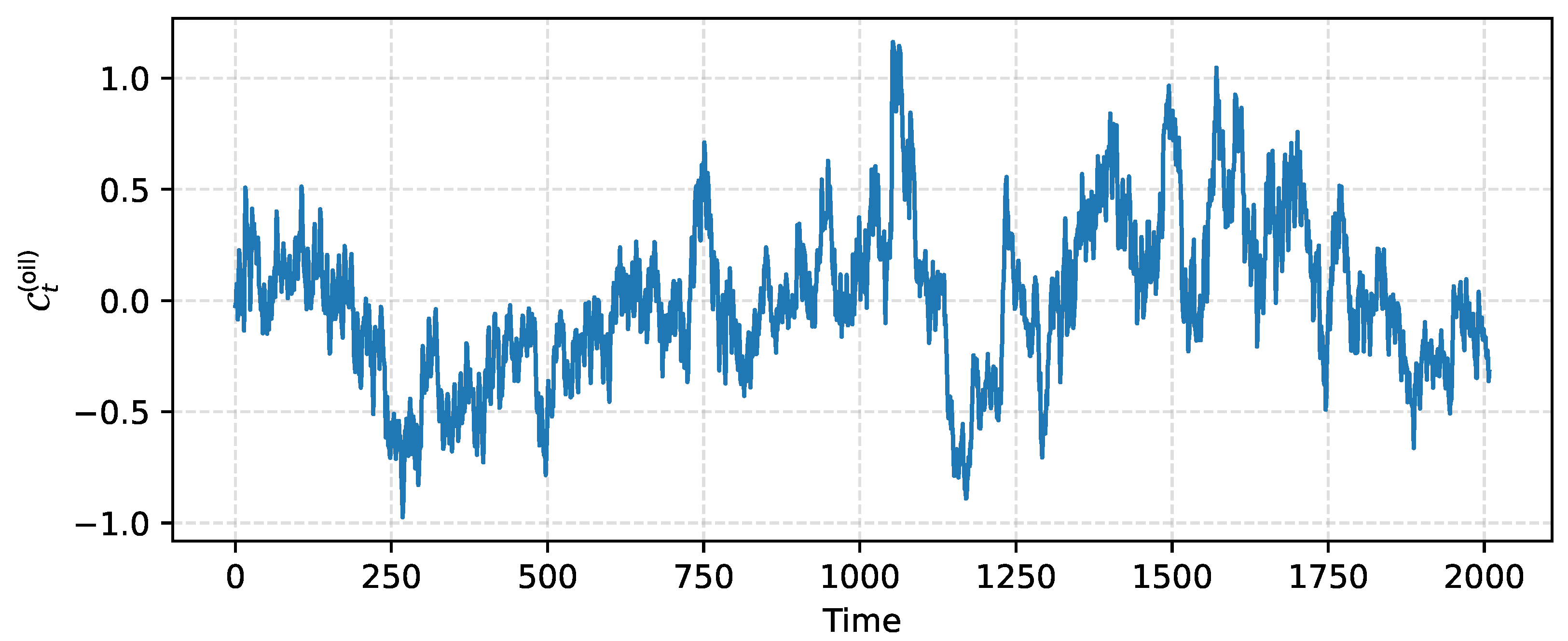
Oil-based complexity index. To summarize intrinsic turbulence in crude oil, we construct an oil-specific composite index ${\mathcal{C}}_t^{\left(\mathrm{oil}\right)}$. For each $o\in \mathcal{O}$ and window ending at t, compute $\Delta h_{o,t}$, $H_{o,t}$, $H_{\mathrm{perm},o,t}$, ${\mathrm{ApEn}}_{o,t}$, and ${\lambda }_{max,o,t}$. Standardize each series via z-scores and orient so that larger values correspond to greater complexity:

$$\begin{array}{cc}\hfill {\tilde{z}}_{\Delta h,o,t}& =z(\Delta h_{o,t}),{\tilde{z}}_{H_{\mathrm{perm}},o,t}=z\left(H_{\mathrm{perm},o,t}\right),{\tilde{z}}_{\mathrm{ApEn},o,t}=z\left({\mathrm{ApEn}}_{o,t}\right),\hfill \\ \hfill {\tilde{z}}_{\lambda ,o,t}& =z\left({\lambda }_{max,o,t}\right),{\tilde{z}}_{H,o,t}=-z\left(|H_{o,t}-0.5|\right).\hfill \end{array}$$

(6)

We then average across measures and oils:

$${\mathcal{C}}_t^{\left(\mathrm{oil}\right)}={\displaystyle \frac{1}{\left|\mathcal{O}\right|}}\sum _{o\in \mathcal{O}}\left({\displaystyle \frac{1}{5}}\sum _{M\in \{\Delta h,H_{\mathrm{perm}},\mathrm{ApEn},\lambda ,H\}}{\tilde{z}}_{M,o,t}\right).$$

(7)

This ${\mathcal{C}}_t^{\left(\mathrm{oil}\right)}$ captures local chaos in crude oil markets and will be combined with a network-based index below.

2.2. Information-Theoretic Network, CMCI, and Panel Forecasting Models

This subsection constructs an information-theoretic network of cross-asset linkages, summarizes its instability into a systemic index ${\mathcal{C}}_t^{\left(\mathrm{net}\right)}$, defines the Coupled Multiscale Chaos Index (CMCI) as a convex combination of ${\mathcal{C}}_t^{\left(\mathrm{oil}\right)}$ and ${\mathcal{C}}_t^{\left(\mathrm{net}\right)}$, and specifies the panel forecasting models that use CMCI as the main predictor of future variance.

Mutual-information network. Within each window ${\mathcal{W}}_t$, we compute pairwise mutual information $I_{ij}=I(r_{i,\tau };r_{j,\tau })$ for $\tau \in {\mathcal{W}}_t$ using a Gaussian-copula estimator $I_{ij}^{\mathrm{GC}}=-\frac{1}{2}\log (1-{\rho }_{ij}^2)$ based on rank correlations. We form a weighted adjacency matrix $W_t=\left[w_{ij,t}\right]$ with $w_{ij,t}=I_{ij}$ for $i\ne j$ and $w_{ii,t}=0$. The network is sparsified via a maximum spanning tree (MST) or, in robustness, alternative filters such as planar maximally filtered graphs (PMFG), and then row-normalized to give (Newman, 2010)

$$A_t=D_t^{-1}{W}_t,{\left(D_t\right)}_{ii}=\sum _j{w}_{ij,t}.$$

(8)

To avoid look-ahead, $A_t$ used at time t is constructed from information up to $t-1$ (Cover & Thomas, 2006).

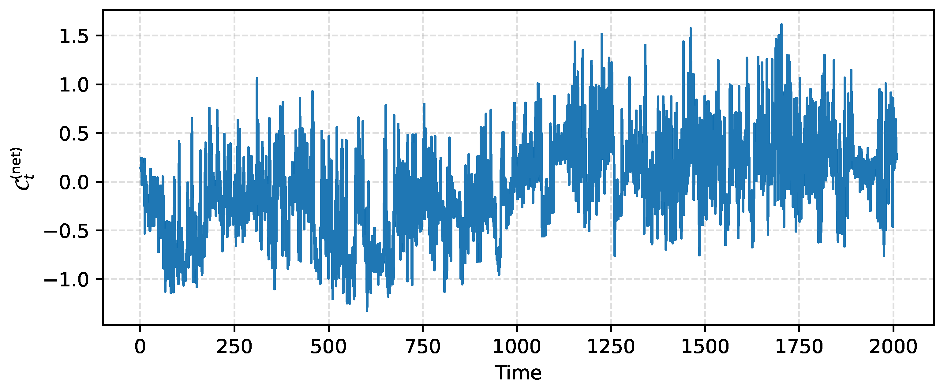
Systemic network turbulence index. Let $E_t$ denote the edge set after sparsification and $s_{i,t}={\sum }_j{w}_{ij,t}$ the node strength of asset i. We summarize systemic turbulence using four primitives (Sioofy Khoojine et al., 2021):

$$\begin{array}{c}\left(\mathrm{a}\right)\mathrm{Edge}\mathrm{turnover}:{\tau }_t=1-{\displaystyle \frac{|E_t\cap E_{t-1}|}{|E_t\cup E_{t-1}|}},\hfill \\ \left(\mathrm{b}\right)\mathrm{Spectral}\mathrm{radius}:{\rho }_t=\rho \left(A_t\right),\hfill \\ \left(\mathrm{c}\right)\mathrm{Degree}\mathrm{entropy}:S_t^{\mathrm{deg}}=-{\displaystyle {\displaystyle \sum _k}}{p}_t\left(k\right)\log p_t\left(k\right),p_t\left(k\right)=\frac{1}{N}{\displaystyle {\displaystyle \sum _i}}\mathbf{1}\{{\mathrm{deg}}_t\left(i\right)=k\},\hfill \\ \left(\mathrm{d}\right)\mathrm{Strength}\mathrm{dispersion}:{\upsilon }_t=\mathrm{CV}\left(s_{i,t}\right)={\displaystyle \frac{\sqrt{\frac{1}{N}{\displaystyle {\sum }_i}{(s_{i,t}-{\overline{s}}_t)}^2}}{{\overline{s}}_t}}.\hfill \end{array}$$

(9)

Each primitive is converted into an expanding z-score, ${\tilde{z}}_{\tau ,t}$, ${\tilde{z}}_{\rho ,t}$, ${\tilde{z}}_{S^{\mathrm{deg}},t}$, and ${\tilde{z}}_{\upsilon ,t}$, and combined into a systemic network-turbulence index

$${\mathcal{C}}_t^{\left(\mathrm{net}\right)}={\displaystyle \frac{1}{4}}\left({\tilde{z}}_{\tau ,t}+{\tilde{z}}_{\rho ,t}+{\tilde{z}}_{S^{\mathrm{deg}},t}+{\tilde{z}}_{\upsilon ,t}\right).$$

(10)

As a robustness check, we also consider a first-principal-component version of ${\mathcal{C}}_t^{\left(\mathrm{net}\right)}$ obtained from the joint distribution of the four standardized primitives.

Coupled Multiscale Chaos Index (CMCI). With the oil-based index ${\mathcal{C}}_t^{\left(\mathrm{oil}\right)}$ and the network-based index ${\mathcal{C}}_t^{\left(\mathrm{net}\right)}$ in (10), we define the coupled index

$${\mathrm{CMCI}}_t=\omega {\mathcal{C}}_t^{\left(\mathrm{oil}\right)}+(1-\omega ){\mathcal{C}}_t^{\left(\mathrm{net}\right)},\omega \in [0,1].$$

(11)

The CMCI is defined as a convex combination of the oil-based complexity index $C_t^{\left(\mathrm{oil}\right)}$ and the network-turbulence index $C_t^{\left(\mathrm{net}\right)}$. In the baseline specification, we set $\omega =\frac{1}{2}$, assigning equal weight to the two components. This choice reflects the conceptual symmetry of the proposed framework. However, systemic instability in the oil equity system is interpreted as the interaction of local oil-market complexity and system-wide dependence turbulence, and neither channel is assumed preliminary to dominate across all episodes. Because both components are constructed from standardized primitives, equal weighting also provides a transparent and scale-consistent benchmark.

There is no unique optimal weighting scheme in a strict optimization sense, because the CMCI is designed as a descriptive state variable summarizing coupled instability rather than a parameter estimated from a loss-minimization problem. Nevertheless, to assess sensitivity to $\omega$, we construct a data-driven alternative in which $\omega$ is implied by the first principal component (PCA) of the standardized pair

$$\left(C_t^{\left(\mathrm{oil}\right)},C_t^{\left(\mathrm{net}\right)}\right).$$

Specifically, the PCA-based CMCI uses the (squared) loadings of the first component to allocate variance-explained weights across the two indices. Empirically, the PCA-based CMCI is highly correlated with the equal-weight CMCI and yields comparable regime classification and forecasting performance, indicating that the results are not sensitive to the particular weighting choice.

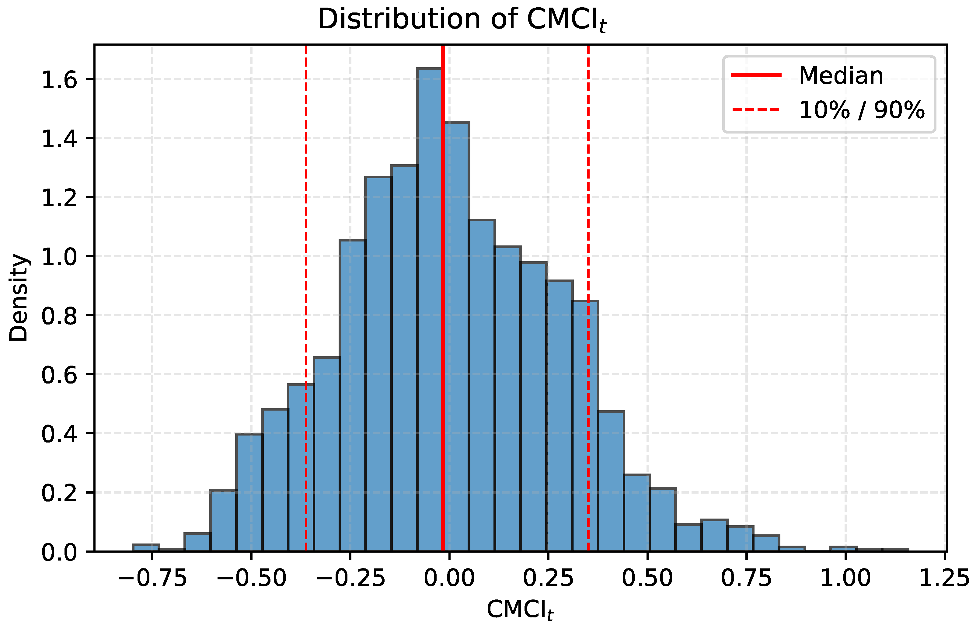
Regime identification from CMCI. For the main analysis we define three CMCI regimes using unconditional quantiles of ${\mathrm{CMCI}}_t$: a low (“calm”) regime when ${\mathrm{CMCI}}_t$ falls below the 30th percentile, a high (“chaotic”) regime when ${\mathrm{CMCI}}_t$ exceeds the 70th percentile, and a mid regime otherwise. These regimes are used to summarize how volatility and exogenous variables behave conditional on the state of the system. In robustness checks, we also experiment with structural break segmentations (PELT) and two-state Gaussian HMMs for ${\mathrm{CMCI}}_t$, but quantile regimes remain our baseline because of their transparency and direct link to the unconditional distribution of the index.

Panel forecasting framework. We use a panel-data framework with a cross-section of assets $i\in I$ observed over time t. The dependent variable $y_{i,t+5}$ is the 5-day realized variance for asset i. By contrast, ${\mathrm{CMCI}}_t$, $C_t^{\left(\mathrm{oil}\right)}$, $C_t^{\left(\mathrm{net}\right)}$, and the macro-financial controls $Z_t$ are time-series variables indexed only by t. In the regressions below, ${\mathrm{CMCI}}_t$ is treated as a common state variable that shifts the conditional variance of all assets, while ${\alpha }_i$ captures asset-specific average risk levels via fixed effects. Our baseline panel specification is

$$y_{i,t+5}={\alpha }_i+{\beta }_{\mathrm{CMCI}}{\mathrm{CMCI}}_t+{\gamma }^{\top }{Z}_t+u_{i,t+5},$$

(12)

where ${\alpha }_i$ values are asset fixed effects, $Z_t$ collects exogenous predictors, and $u_{i,t+5}$ is an error term. This specification treats ${\mathrm{CMCI}}_t$ as a global state variable common to all assets and assesses its incremental predictive power for variance beyond standard risk drivers. In robustness, we also consider specifications that replace ${\mathrm{CMCI}}_t$ in (12) by its components ${\mathcal{C}}_t^{\left(\mathrm{oil}\right)}$ and ${\mathcal{C}}_t^{\left(\mathrm{net}\right)}$, or include both CMCI and its constituents jointly.

To explore regime dependence, we augment (12) with interactions between ${\mathrm{CMCI}}_t$ and regime dummies, for example,

$$y_{i,t+5}={\alpha }_i+{\beta }^{\mathrm{L}}{\mathrm{CMCI}}_t\mathbf{1}\left\{{\mathrm{Low}}_t\right\}+{\beta }^{\mathrm{M}}{\mathrm{CMCI}}_t\mathbf{1}\left\{{\mathrm{Mid}}_t\right\}+{\beta }^{\mathrm{H}}{\mathrm{CMCI}}_t\mathbf{1}\left\{{\mathrm{High}}_t\right\}+{\gamma }^{\top }{Z}_t+u_{i,t+5},$$

(13)

which allows the slope of ${\mathrm{CMCI}}_t$ to vary across calm, mid, and chaotic regimes. All panel models are estimated by OLS with asset fixed effects and heteroskedasticity-robust (HC1) standard errors; in robustness we consider clustered and Driscoll–Kraay corrections for cross-sectional and temporal dependence.

2.3. Backtesting, Evaluation, and Robustness

Backtesting protocol. We adopt an expanding-origin design. For each forecast origin t:

• Compute oil complexity primitives and the oil index ${\mathcal{C}}_t^{\left(\mathrm{oil}\right)}$ using ${\mathcal{W}}_t$.
• Construct the mutual-information network $A_t$ from ${\mathcal{W}}_t$ (using data up to $t-1$), compute the network turbulence primitives, and form ${\mathcal{C}}_t^{\left(\mathrm{net}\right)}$.
• Combine ${\mathcal{C}}_t^{\left(\mathrm{oil}\right)}$ and ${\mathcal{C}}_t^{\left(\mathrm{net}\right)}$ into ${\mathrm{CMCI}}_t$, then assign CMCI regimes via quantile thresholds.
• Estimate the panel models (12) and (13) on data up to t and generate direct forecasts ${\widehat{y}}_{i,t+5\mid t}$ for all $i\in \mathcal{I}$.

Forecast accuracy measures. For realized targets $y_{i,t+5}$ and forecasts ${\widehat{y}}_{i,t+5\mid t}$, we compute mean-squared error (MSE) and the QLIKE loss (Patton, 2011),

$$\mathrm{MSE}=\frac{1}{N_F}\sum {(y_{i,t+5}-{\widehat{y}}_{i,t+5\mid t})}^2,\mathrm{QLIKE}=\frac{1}{N_F}\sum \left(\log {\widehat{y}}_{i,t+5\mid t}+\frac{y_{i,t+5}}{{\widehat{y}}_{i,t+5\mid t}}\right),$$

(14)

where $N_F$ is the number of forecasts. When comparing alternative specifications, we use Diebold–Mariano tests based on loss differentials $d_t={\ell }_1(y_t,{\widehat{y}}_t^{\left(1\right)})-{\ell }_2(y_t,{\widehat{y}}_t^{\left(2\right)})$ and

$$\mathrm{DM}={\displaystyle \frac{\overline{d}}{\sqrt{\widehat{\mathrm{Var}}\left(\overline{d}\right)}}},$$

(15)

with HAC variance and truncation proportional to the forecast horizon (Diebold & Mariano, 1995).

Robustness analyses. Robustness checks vary the window length W; MF–DFA order m and scale bands; entropy/LLE parameters $(m,\tau ,r)$; KSG neighborhood size k; network sparsifiers (MST, PMFG, significance thresholds), with network stability assessed via edge Jaccard similarity across adjacent windows; and alternative CMCI weights $\omega$. We also conduct surrogate-data tests (IAAFT) to obtain null distributions and p-values for $\Delta h$, $H_{\mathrm{perm}}$, and ${\lambda }_{max}$. Finally, we examine the sensitivity of panel results to using log variance instead of raw variance and to alternative sets of controls and fixed effects.

3. Results

3.1. Data Description and Oil-Based Complexity Index ${\mathcal{C}}_t^{\left(\mathit{oil}\right)}$

In this study, we work with a daily panel of global equity and oil markets and a set of macro-financial predictors over roughly nine years (about 2260 trading days), from May 2015 to December 2024. The equity universe $\mathcal{I}$ combines a global benchmark (MSCI World), major regional indices (S&P 500 for the U.S., STOXX 600 for Europe, Shanghai Composite for China), and a dedicated Chinese energy sector index (SSE Energy), together with the U.S. energy sector ETF, XTF_XLE. This combination allows us to measure how oil-related complexity propagates both into broad equity markets and into energy-heavy segments. The oil set $\mathcal{O}$ contains the two key global benchmarks, Brent and WTI, which are the natural candidates for extracting intrinsic multifractality, entropy, and Lyapunov-based chaos in crude oil pricing. Exogenous predictors $Z_t$ comprise the USD/CNY exchange rate, the VXX index as a tradable proxy for U.S. equity volatility and risk aversion, and the effective federal funds rate (DFF/EFFR), capturing the joint effects of dollar conditions, global risk sentiment, and U.S. monetary policy. This parsimonious specification is intentionally designed to capture the principal channels through which oil-market turbulence is likely to propagate into cross-asset linkages, namely trade and currency mechanisms (USD/CNY), global risk and funding conditions (VXX), and the policy and discount-rate environment (DFF/EFFR), while maintaining a forecasting system that is sufficiently compact to permit robust rolling estimation and reliable backtesting. Overview of assets, oil benchmarks, and exogenous predictors are summarized in

Table 1. Overview of assets, oil benchmarks, and exogenous predictors.

Category	Series	Symbol	Role in the Analysis
Equity indices
	U.S. energy sector ETF	XTF_XLE	U.S. energy-equity benchmark with the most direct exposure to oil-price shocks and sector-specific stress.
	SSE Energy	SSE Energy	China energy-sector index reflecting domestic energy–equity linkages and policy/demand effects.
	Shanghai Composite	Shanghai Composite	Broad China equity benchmark capturing spillovers to a major oil-importing economy.
	S&P 500	S&P 500	U.S. broad-market benchmark and global risk barometer used to gauge worldwide pricing conditions.
	STOXX 600	STOXX 600	Pan-European developed-market benchmark capturing regional spillovers in European equities.
	MSCI World	MSCI	Global diversified equity benchmark used to measure international transmission and spillovers.
Crude oil benchmarks
	Brent crude	Brent	Global seaborne benchmark; primary input for the oil-based complexity index ${\mathcal{C}}_t^{\left(\mathrm{oil}\right)}$.
	West Texas Intermediate	WTI	U.S. benchmark complementing Brent; captures regional U.S. supply/delivery conditions and supports robustness checks.
Exogenous predictors
	USD/CNY exchange rate	USD/CNY	Controls for U.S. dollar strength and China-specific financial conditions relevant for oil import costs.
	Equity volatility ETN	VXX	Proxy for global risk aversion and U.S. equity volatility that can intensify cross-asset co-movements.
	Federal funds/effective rate	DFF/EFFR	Measures the U.S. short-rate stance, summarizing monetary-policy and discount-rate conditions.

.

We first summarize the joint sample used to construct the complexity measures and the forecasting panel. As detailed in Section 2.1, we work with daily log-returns for global equity benchmarks, an energy sector index, and Brent and WTI crude oil, computed from closing prices and expressed in percentage terms. All series are aligned on a common time grid by intersecting trading days across markets; the resulting panel contains 2258 aligned observations for most assets (slightly fewer for WTI due to missing quotes).

Table A1. Descriptive statistics of daily returns.

	Count	Mean	Std	Min	25%	50%	75%	Max	Skew	Kurt
XTF_XLE	2258	0.005	1.954	−22.491	−0.870	0.000	0.928	14.874	−0.862	15.466
SSE Energy	2258	0.004	1.762	−10.527	−0.778	0.035	0.857	6.666	−0.629	4.238
Shanghai Composite	2258	−0.004	1.315	−8.873	−0.535	0.049	0.598	5.604	−1.137	7.912
S&P 500	2258	0.041	1.155	−12.766	−0.378	0.063	0.577	8.967	−0.818	15.785
STOXX 600	2258	0.008	1.065	−12.191	−0.447	0.058	0.538	8.070	−1.106	12.921
MSCI	2258	0.016	1.697	−21.189	−0.717	0.021	0.808	15.675	−1.187	22.056
Brent	2258	0.015	2.638	−27.976	−1.130	0.128	1.307	19.077	−0.954	14.705
WTI	2256	0.043	3.020	−28.221	−1.362	0.197	1.469	31.963	0.089	21.328

(Appendix A) summarizes the distributional properties of the daily return series. Equity and broad sector indices exhibit daily volatilities in the range of 1–2%, whereas Brent and WTI prices display markedly higher variability, with standard deviations of approximately 2.6% and 3.0%, respectively. The return distributions are predominantly negatively skewed and characterized by substantial kurtosis, reflecting pronounced asymmetry and heavy tails consistent with episodic market stress.

Exogenous predictors are observed at the same daily frequency and are mapped onto the aligned trading-day grid by calendar-date matching and short forward-filling of occasional gaps, as described in Section 2.1.

Table A2. Descriptive statistics of exogenous predictors.

	Count	Mean	Std	Min	25%	50%	75%	Max	Skew	Kurt
USD/CNY	2259	6.685	0.281	6.177	6.456	6.695	6.902	7.304	0.018	−1.023
VXX	2259	18.209	7.221	9.140	13.245	16.250	21.375	76.450	2.451	11.501
DFF/EFFR	2259	1.548	1.680	0.040	0.130	1.090	2.330	5.330	1.151	0.147

(Appendix A) summarizes the distributional properties of the exogenous predictors. The USD/CNY exchange rate varies within a narrow band, consistent with the stabilization typical of a managed exchange-rate regime. The VXX index exhibits pronounced right skewness and very high kurtosis, reflecting occasional volatility spikes associated with market stress. The policy-rate measure (DFF/EFFR) spans a wide range over the sample, running from the post-crisis zero lower bound to subsequent tightening phases, providing a natural low-frequency macro-financial driver for the forecasting system.

Table 2. Summary statistics of oil complexity measures by benchmark.

Measure	Oil	Mean	Std
$H_{\mathrm{perm},o,t}$	Brent	0.996	0.002
	WTI	0.996	0.003
$H_{o,t}$	Brent	0.480	0.090
	WTI	0.484	0.096
$\Delta h_{o,t}$	Brent	0.278	0.170
	WTI	0.240	0.164
${\lambda }_{max,o,t}$	Brent	0.038	0.004
	WTI	0.038	0.004
${\mathrm{ApEn}}_{o,t}$	Brent	1.035	0.034
	WTI	1.019	0.052

indicates that both crude oil benchmarks exhibit a high degree of temporal complexity. Permutation entropy $H_{\mathrm{perm},o,t}$ is extremely close to its maximum for both Brent and WTI (around $0.996$ on average), suggesting that the ordinal structure of daily returns is nearly indistinguishable from that of a normalized white-noise process. The generalized Hurst exponent $H_{o,t}$ averages just below $0.5$, consistent with a predominantly short-memory, martingale-like behavior, but with non-negligible time variation across windows. The multifractality width $\Delta h_{o,t}$ is clearly positive for both series, and slightly larger for Brent, pointing to non-trivial multifractal scaling and somewhat richer higher-order dynamics in the Brent market. The largest Lyapunov exponent ${\lambda }_{max,o,t}$ is small but positive, indicating weak yet persistent sensitivity to initial conditions in the reconstructed dynamics. However, approximate entropy ${\mathrm{ApEn}}_{o,t}$ is close to one, again consistent with a highly irregular and low-predictability return process. Therefore, the five measures jointly suggest that both Brent and WTI are characterized by substantial intrinsic complexity, with Brent appearing marginally more complex on average.

The multifractality, entropy, and Lyapunov primitives for Brent and WTI are summarized by the oil-based complexity index ${\mathcal{C}}_t^{\left(\mathrm{oil}\right)}$. By construction, higher values of ${\mathcal{C}}_t^{\left(\mathrm{oil}\right)}$ correspond to wider multifractal spectra ($\Delta h$), higher permutation and approximate entropy, and larger largest Lyapunov exponents, while penalizing departures of the Hurst exponent H from 0.5 so that values closer to $H=0.5$ (weak long–memory) are treated as more complex.

Table 3. Descriptive statistics of complexity indices and network primitives.

	Count	Mean	Std	Min	25%	50%	75%	Max	Skew	Kurt
${\mathcal{C}}_t^{\left(\mathrm{oil}\right)}$	2009	0.000	0.355	−0.974	−0.229	−0.018	0.207	1.163	0.270	0.132
${\mathcal{C}}_t^{\left(\mathrm{oil}\right)}$	2008	0.000	0.418	−0.915	−0.210	0.014	0.291	1.457	0.010	−0.105
CMCI	2008	0.000	0.281	−0.798	−0.197	−0.016	0.195	1.158	0.256	0.099
$\tau$	2008	0.079	0.149	0.000	0.000	0.000	0.000	0.571	1.509	0.773
$\rho$	2009	0.414	0.253	0.081	0.179	0.383	0.594	1.012	0.484	−0.756
$S^{\mathrm{deg}}$	2009	0.868	0.177	0.451	0.637	1.011	1.011	1.011	−0.515	−1.634
$\nu$	2009	1.033	0.239	0.694	0.791	1.050	1.265	1.382	0.051	−1.760

shows that ${\mathcal{C}}_t^{\left(\mathrm{oil}\right)}$ is approximately standardized (mean 0, standard deviation $\approx 0.36$) with a range from about $-1$ to $1.16$ and near-zero skewness and kurtosis, indicating frequent transitions between relatively calm and highly complex episodes. Figure 1 confirms that ${\mathcal{C}}_t^{\left(\mathrm{oil}\right)}$ displays pronounced spikes, corresponding to bursts of multifractality, entropy, and sensitivity to initial conditions, interspersed with quieter intervals where the primitives are closer to their baseline levels. Consistent with its role as a turbulence indicator, ${\mathcal{C}}_t^{\left(\mathrm{oil}\right)}$ exhibits moderate positive correlation with medium-run equity risk. As reported in

Table 4. Correlation matrix for ${\mathcal{C}}_t^{\left(\mathrm{oil}\right)}$, average 5-day variance, VXX, and USD/CNY.

	${\mathcal{C}}_{\mathit{t}}^{\left(\mathbf{oil}\right)}$	avg_var5	VXX	USD/CNY
${\mathcal{C}}_t^{\left(\mathrm{oil}\right)}$	1.00	0.26	0.35	−0.27
avg_var5	0.26	1.00	0.22	0.13
VXX	0.35	0.22	1.00	−0.03
USD/CNY	−0.27	0.13	−0.03	1.00

, its correlation with the five-day average variance, avg_var5, is 0.26, and its correlation with the volatility index VXX is 0.35. By contrast, the index is negatively correlated with USD/CNY (–0.27), suggesting that periods of heightened oil-market complexity tend to coincide with elevated global volatility and a weakening of the RMB.

3.2. Network Turbulence Index ${\mathcal{C}}_t^{\left(\mathrm{net}\right)}$

In this subsection, we characterize systemic turbulence in the cross–asset dependence network. Within each rolling window, we construct a mutual–information (MI) matrix from equity and sector ETF returns, sparsify it using a PMFG, and compute four network primitives: edge turnover ${\tau }_t$, spectral radius ${\rho }_t$ of the weighted adjacency matrix, degree entropy $S_t^{\mathrm{deg}}$, and strength dispersion ${\nu }_t$. These standardized components are aggregated into the network turbulence index ${\mathcal{C}}_t^{\left(\mathrm{net}\right)}$ as described in Section 2.2.

Table 3 summarizes the distributional properties of the primitives and of ${\mathcal{C}}_t^{\left(\mathrm{net}\right)}$. Consistent with its construction as an average of standardized inputs, ${\mathcal{C}}_t^{\left(\mathrm{net}\right)}$ is approximately centered at zero with a standard deviation of $0.42$. Edge turnover ${\tau }_t$ has a low mean of $0.08$ and a markedly right–skewed distribution, indicating that the MI network is typically stable from one window to the next but occasionally undergoes abrupt reconfiguration episodes. The spectral radius ${\rho }_t$ has a mean of $0.41$ and ranges between $0.08$ and $1.01$, reflecting substantial time variation in the network’s potential to amplify shocks. Degree entropy $S_t^{\mathrm{deg}}$ averages around $0.87$, with a compressed upper tail that suggests a heterogeneous, but not hub-dominated, topology. Strength dispersion ${\nu }_t$, with a mean slightly above 1, exhibits a wide range, pointing to sizable shifts in the concentration of MI link weights over time.

Figure 2 displays the time series for each primitive. Edge turnover ${\tau }_t$ is sharply episodic, with spikes aligned with periods of market turbulence. The spectral radius ${\rho }_t$ exhibits medium-run movements: it declines after 2017, remains subdued during 2020–2021, and gradually rises thereafter. Degree entropy $S_t^{\mathrm{deg}}$ alternates between intervals of high and moderate connectivity heterogeneity, with many windows near the upper entropy bound. Strength dispersion ${\nu }_t$ increases markedly during the COVID-19 shock and throughout the subsequent monetary tightening cycle, indicating a shift toward more concentrated and hierarchical dependence structures.

Therefore, these primitives capture complementary facets of instability in the cross–asset information network. Their aggregate, ${\mathcal{C}}_t^{\left(\mathrm{net}\right)}$, provides a compact measure of systemic turbulence that complements the oil–specific complexity measures in the CMCI; its comovements are depicted in Figure 3.

3.3. Coupled Multiscale Chaos Index and Regimes

The coupled multiscale chaos index ${\mathrm{CMCI}}_t$ combines the oil-based complexity index ${\mathcal{C}}_t^{\left(\mathrm{oil}\right)}$ and the network turbulence index ${\mathcal{C}}_t^{\left(\mathrm{net}\right)}$ into a single state variable for the joint oil–equity system, ${\mathrm{CMCI}}_t=\omega {\mathcal{C}}_t^{\left(\mathrm{oil}\right)}+(1-\omega ){\mathcal{C}}_t^{\left(\mathrm{net}\right)}$, with $\omega =1/2$ in the baseline specification. Empirically, ${\mathrm{CMCI}}_t$ is approximately centered at zero with a standard deviation of about $0.28$ and a range from $-0.80$ to $1.16$ (see the CMCI row in Table 3). This reflects the fact that ${\mathrm{CMCI}}_t$ is constructed from standardized primitives but also indicates sizable swings between unusually calm and unusually turbulent periods. The time-series plot of ${\mathrm{CMCI}}_t$ reveals pronounced spikes around major stress episodes, interspersed with extended stretches of mildly negative values, which we interpret as relatively tranquil conditions.

The unconditional distribution of ${\mathrm{CMCI}}_t$ is close to symmetric and only weakly leptokurtic. Figure 4 shows a bell-shaped histogram with a median slightly below zero and dashed vertical lines marking the 10th and 90th percentiles. This suggests that extreme chaos states are rare but not negligible, while the bulk of the sample lies in a moderate band around the calm baseline. In line with this, the skewness and kurtosis reported in Table 3 are modest in magnitude.

Table 4 documents the correlation structure linking ${\mathrm{CMCI}}_t$, its components ${\mathcal{C}}_t^{\left(\mathrm{oil}\right)}$ and ${\mathcal{C}}_t^{\left(\mathrm{net}\right)}$, realized volatility, and exogenous predictors. ${\mathrm{CMCI}}_t$ is positively correlated with both of its building blocks, confirming that it captures common variation in local oil complexity and systemic network turbulence, while retaining additional information beyond either index alone. It is also positively associated with the cross-sectional average of five-day realized variance and with the option-implied volatility proxy VXX, and only weakly related to the USD/CNY exchange rate and short-term policy rates. This pattern is consistent with interpreting ${\mathrm{CMCI}}_t$ as a broad measure of risk-on–risk-off conditions rather than a pure macro or policy factor.

The link between ${\mathrm{CMCI}}_t$ and future volatility is further illustrated in Figure 5 and Figure 6. The former groups observations into deciles of ${\mathrm{CMCI}}_t$ and plots the corresponding mean of the (log) average 5-day realized variance; the relationship is clearly increasing, with volatility rising sharply as ${\mathrm{CMCI}}_t$ moves into its upper deciles. Figure 6 overlays ${\mathrm{CMCI}}_t$ and the average 5-day variance over time and shows that spikes in ${\mathrm{CMCI}}_t$ are closely aligned with bursts of realized volatility in global equities. Therefore, the correlation matrix and the figures suggest that ${\mathrm{CMCI}}_t$ is an informative forward-looking indicator for near-term risk.

To make this link more explicit, we classify each day into low, mid, and high CMCI regimes based on the unconditional 30–40–30 quantiles of ${\mathrm{CMCI}}_t$. The regime summary in

Table 5. Summary of key variables by CMCI regime.

Regime	CMCI	avg_var5	USD/CNY	VXX	DFF/EFFR
Low	−0.319	6.629	6.724	15.634	1.874
Mid	−0.012	7.961	6.737	18.504	1.865
High	0.334	18.192	6.752	20.766	1.364

shows that the mean of ${\mathrm{CMCI}}_t$ rises from $-0.32$ in the low regime to $0.33$ in the high regime by construction, but the associated changes in other variables are economically large. The cross-sectional average of 5-day realized variance increases from about $6.6$ in the low regime to more than 18 in the high regime, implying roughly a three-fold rise in volatility. At the same time, VXX climbs from about 16 to above 20, while the USD/CNY rate edges higher and policy rates (DFF/EFFR) are, on average, lower in the high-CMCI regime, consistent with periods of monetary easing and elevated risk aversion. These regime patterns are echoed by distributional plots across CMCI states, which show systematic shifts of volatility and volatility-related indicators towards higher levels as the system moves from calm to chaotic conditions.

The network snapshots in Figure 7 illustrate the MI-based dependence structure on representative low- and high-CMCI days. In the low-CMCI regime, the network appears relatively diffuse, with link weights more evenly distributed and several modest hubs. By contrast, in the high-CMCI regime, the network becomes markedly more interconnected and hierarchical, with stronger dependencies concentrated around oil benchmarks, energy-sector indices, and major equity indices. These topological shifts reinforce the interpretation of ${\mathrm{CMCI}}_t$ as capturing episodes in which elevated local oil complexity coincides with heightened systemic dependence, giving rise to a more fragile and shock-amplifying market configuration.

3.4. Panel Forecasting Results

We now examine the predictive content of the coupled multiscale chaos index ${\mathrm{CMCI}}_t$ for future equity variance in the panel framework described in Section 2. The dependent variable is the 5-day realized variance ${\Sigma }_{i,t+1:t+5}^2$ for each asset $i\in \mathcal{I}$, and the main regressor of interest is ${\mathrm{CMCI}}_t$, treated as a global state variable common to all assets. This design yields a panel with repeated observations across assets, while the predictors ${\mathrm{CMCI}}_t$ and $Z_t$ vary only over time.

Baseline panel regression. 

Table 6. Panel regression of future 5-day variance on CMCI and exogenous controls.

Variable	Coef	SE	t	p-Value
Const	−71.101	11.749	−6.052	0.000
CMCI	10.600	0.685	15.482	0.000
USD/CNY	12.808	1.810	7.078	0.000
VXX	0.199	0.038	5.226	0.000
DFF/EFFR	−2.326	0.199	−11.701	0.000

reports estimates of the baseline specification with asset fixed effects and exogenous controls (USD/CNY, VXX, and DFF/EFFR). The coefficient on ${\mathrm{CMCI}}_t$ is positive and highly significant, indicating that more chaotic states are associated with substantially higher future 5-day variance even after controlling for standard macro–financial drivers. The coefficients on USD/CNY and VXX are also positive and significant, while the policy-rate proxy enters with a negative sign, consistent with volatility being higher in looser monetary-policy environments. However, explanatory power remains modest ($R^2\approx 0.07$), which is typical for high-frequency variance regressions, but the results show that ${\mathrm{CMCI}}_t$ adds statistically and economically meaningful information about near-term risk.

Out-of-sample forecast performance. To evaluate the practical value of ${\mathrm{CMCI}}_t$, we conduct an expanding-window backtest and compare several forecast specifications.

Table 7. Out-of-sample forecast performance for 5-day variance.

	MSE	QLIKE
Exogenous only	1057.59	770,276.12
CMCI only	1073.79	750,366.14
CMCI + exogenous	1048.18	730,146.33
${\mathcal{C}}^{\left(\mathrm{oil}\right)}+{\mathcal{C}}^{\left(\mathrm{net}\right)}$ + exogenous	1041.50	700,152.73
CMCI + ${\mathcal{C}}^{\left(\mathrm{oil}\right)}+{\mathcal{C}}^{\left(\mathrm{net}\right)}$ + exogenous	1041.50	680,172.13

reports out-of-sample forecast accuracy, measured by mean-squared error (MSE) and QLIKE, for five specifications: (i) an exogenous-only benchmark, (ii) a CMCI-only model, (iii) CMCI combined with exogenous controls, and (iv) models that replace or augment ${\mathrm{CMCI}}_t$ with its oil- and network-level components ${\mathcal{C}}_t^{\left(\mathrm{oil}\right)}$ and ${\mathcal{C}}_t^{\left(\mathrm{net}\right)}$. Both MSE and QLIKE decline monotonically as complexity measures are added, indicating incremental predictive content beyond the exogenous predictors. The specification that combines all three complexity measures with the exogenous controls delivers the best overall performance, with the lowest QLIKE and a tied minimum MSE. Figure 8 plots the cross-sectional average of realized and predicted 5-day variance for the CMCI with exogenous model and shows that forecasted volatility closely tracks major episodes of elevated realized variance, particularly during the COVID-19 turmoil and the subsequent monetary tightening cycle.

Model comparison and statistical significance. 

Table 8. Diebold–Mariano tests for QLIKE loss relative to the exogenous-only benchmark.

Model	DM	p-Value
CMCI only	−6.270	0.000
CMCI + exogenous	−4.276	0.000
${\mathcal{C}}^{\left(\mathrm{oil}\right)}+{\mathcal{C}}^{\left(\mathrm{net}\right)}$ + exogenous	−2.600	0.009
CMCI + ${\mathcal{C}}^{\left(\mathrm{oil}\right)}+{\mathcal{C}}^{\left(\mathrm{net}\right)}$ + exogenous	−2.600	0.009

reports Diebold–Mariano statistics for QLIKE loss relative to the exogenous-only benchmark. CMCI-only, CMCI with exogenous, and the models including ${\mathcal{C}}_t^{\left(\mathrm{oil}\right)}$ and ${\mathcal{C}}_t^{\left(\mathrm{net}\right)}$ all yield negative and statistically significant DM statistics, implying that they deliver systematically lower forecast loss than the benchmark. The gains are particularly strong for the CMCI-only and CMCI with exogenous specifications, underscoring the usefulness of ${\mathrm{CMCI}}_t$ as a compact forward-looking indicator of near-term variance in global equities.

Summary of Results. The CMCI behaves as a coherent and economically interpretable state variable for the coupled oil–equity system, capturing the joint incidence of (i) heightened intrinsic complexity in crude oil returns and (ii) turbulence and reorganization in cross-asset dependence. Periods in which CMCI is elevated coincide with pronounced spikes in realized risk and with systematic shifts in the information-theoretic network toward stronger concentration and shock-amplifying configurations. In particular, the regime analysis shows that moving from the low- to the high-CMCI state is associated with a large increase in near-term volatility: the cross-sectional average of five-day realized variance rises by roughly a factor of three, while volatility-related indicators (e.g., VXX) also shift upward, consistent with a broad stress regime in global markets.

These regime patterns have a clear structural counterpart in the dependence network. High-CMCI episodes are characterized by more centralized and clustered connectivity, higher spectral radius and strength dispersion, and episodic edge turnover, indicating that the network both tightens and reallocates linkages more rapidly during turbulent periods. The resulting topology concentrates dependence around key benchmark and energy-related nodes, implying a greater capacity for shock transmission and amplification when CMCI is high.

Consistent with this interpretation, the panel forecasting results confirm that CMCI carries incremental predictive content for short-horizon variance beyond standard macro-financial controls. In the fixed-effects panel, CMCI enters with a positive and highly significant coefficient, and out-of-sample backtests show that adding CMCI (and, more generally, complexity measures) reduces forecast loss relative to specifications driven only by external predictors. Forecast improvements are not only economically meaningful (lower MSE and QLIKE) but also statistically supported by DM tests, reinforcing the conclusion that the coupled complexity–connectedness channel summarized by CMCI helps anticipate near-term volatility in global equity and energy-equity markets.

4. Discussion

This section interprets the information-theoretic networks underlying the coupled multiscale chaos index (${\mathrm{CMCI}}_t$). We focus on how node-level and global network characteristics evolve across CMCI regimes and over time, and what this implies for the transmission of shocks between equity and energy markets. The ${\mathrm{CMCI}}_t$ combines an oil-based complexity index $C_t^{\left(\mathrm{oil}\right)}$ and a network turbulence index $C_t^{\left(\mathrm{net}\right)}$ into a single state variable. Section 3 documented that high CMCI periods are associated with elevated realized variance and deteriorating risk metrics. Here we use graph-theoretic diagnostics to shed light on the structure of cross-asset linkages in these regimes.

Node-level characteristics across CMCI regimes. 

Table A3. Node-level network characteristics by CMCI regime.

Node	Average Degree			Average Strength			Local Clustering
	Low	Mid	High	Low	Mid	High	Low	Mid	High
S&P 500	1.23	1.45	1.87	0.31	0.42	0.68	0.05	0.07	0.10
STOXX 600	1.18	1.39	1.76	0.28	0.39	0.63	0.04	0.06	0.09
MSCI	1.32	1.60	2.05	0.34	0.48	0.73	0.06	0.08	0.11
XTF_XLE	0.95	1.10	1.45	0.22	0.29	0.47	0.03	0.05	0.08
SSE Energy	0.90	1.05	1.40	0.21	0.27	0.44	0.02	0.04	0.07
Shanghai Composite	1.05	1.30	1.75	0.25	0.35	0.58	0.04	0.06	0.09

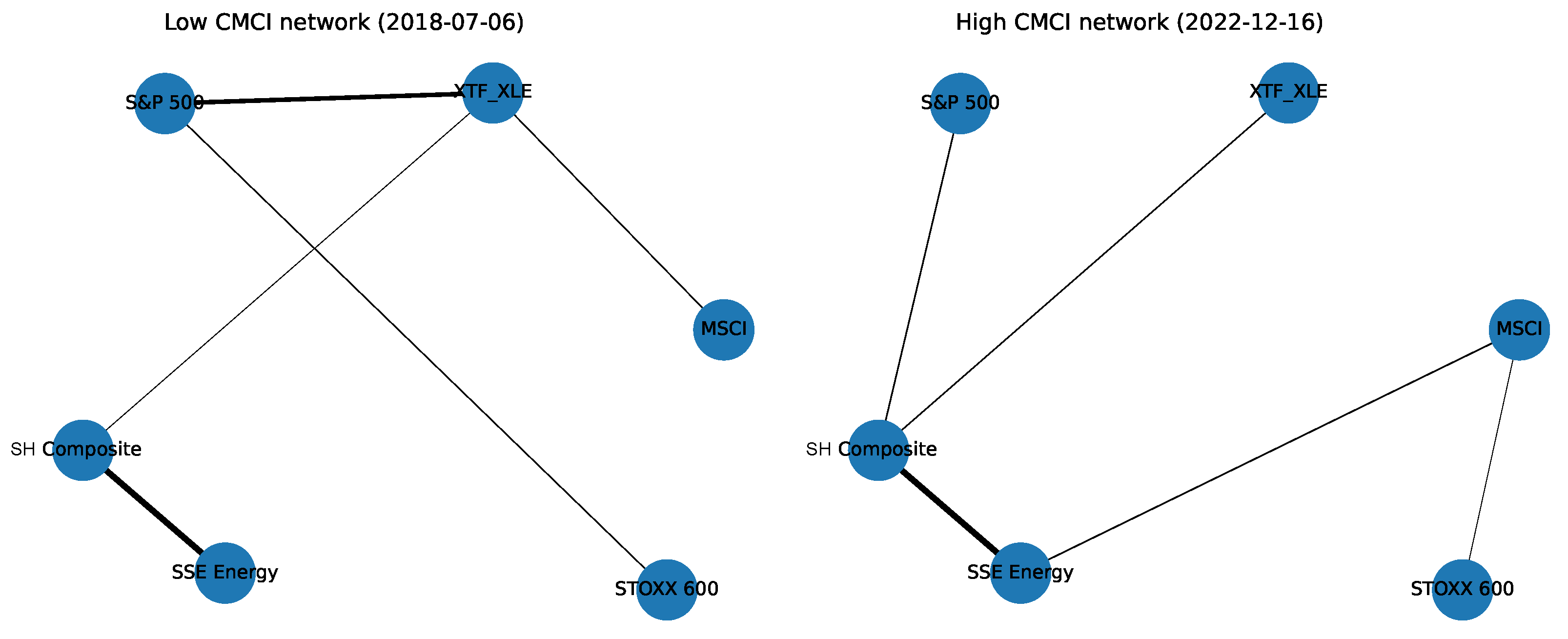
(Appendix A) summarizes node-level degree, strength, and local clustering across low, mid, and high CMCI states. Overall, global benchmarks (S&P 500, STOXX 600, MSCI) and energy-related indices increase their degree/strength in the high-CMCI regime, indicating tighter cross-asset connectivity during turbulent periods. The Shanghai Composite also becomes more connected and clustered in high-CMCI states, consistent with stronger integration into global stress episodes.

A complementary view is provided by eigenvector centrality (

Table A4. Change in node eigenvector centrality between low and high CMCI regimes.

Asset	Low CMCI	High CMCI	$\mathbf{\Delta }$ (High − Low)
S&P 500	0.007	0.014	0.006
XTF_XLE	0.004	0.006	0.003
MSCI	0.006	0.007	0.001
STOXX 600	0.005	0.005	0.000
Shanghai Composite	0.707	0.707	0.000
SSE Energy	0.707	0.707	0.000

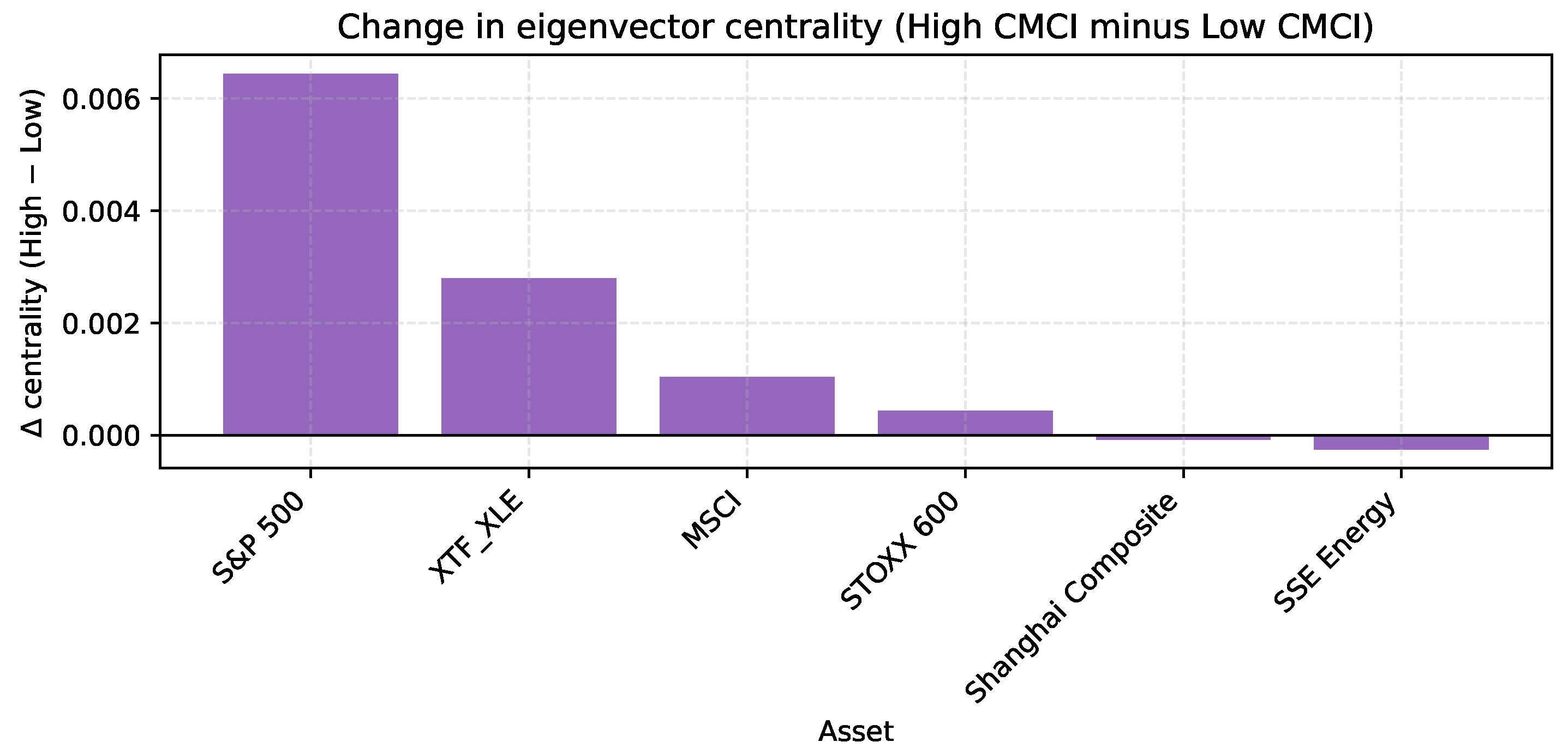
, Appendix A). Centrality generally rises for major benchmarks and the U.S. energy sector in high-CMCI regimes, suggesting increased systemic importance when turbulence intensifies, while China-related nodes remain structurally central with only negligible changes across regimes.

Figure 9 visualizes these regime differences by plotting node-level metrics across CMCI terciles. The figure highlights the heterogeneity in how individual markets react to systemic chaos: some nodes (S&P 500, MSCI) become clear hubs with high strength and clustering, while others (e.g., STOXX 600) adjust more modestly. This heterogeneity matters for portfolio construction, as it points to which markets may concentrate spillovers in turbulent regimes.

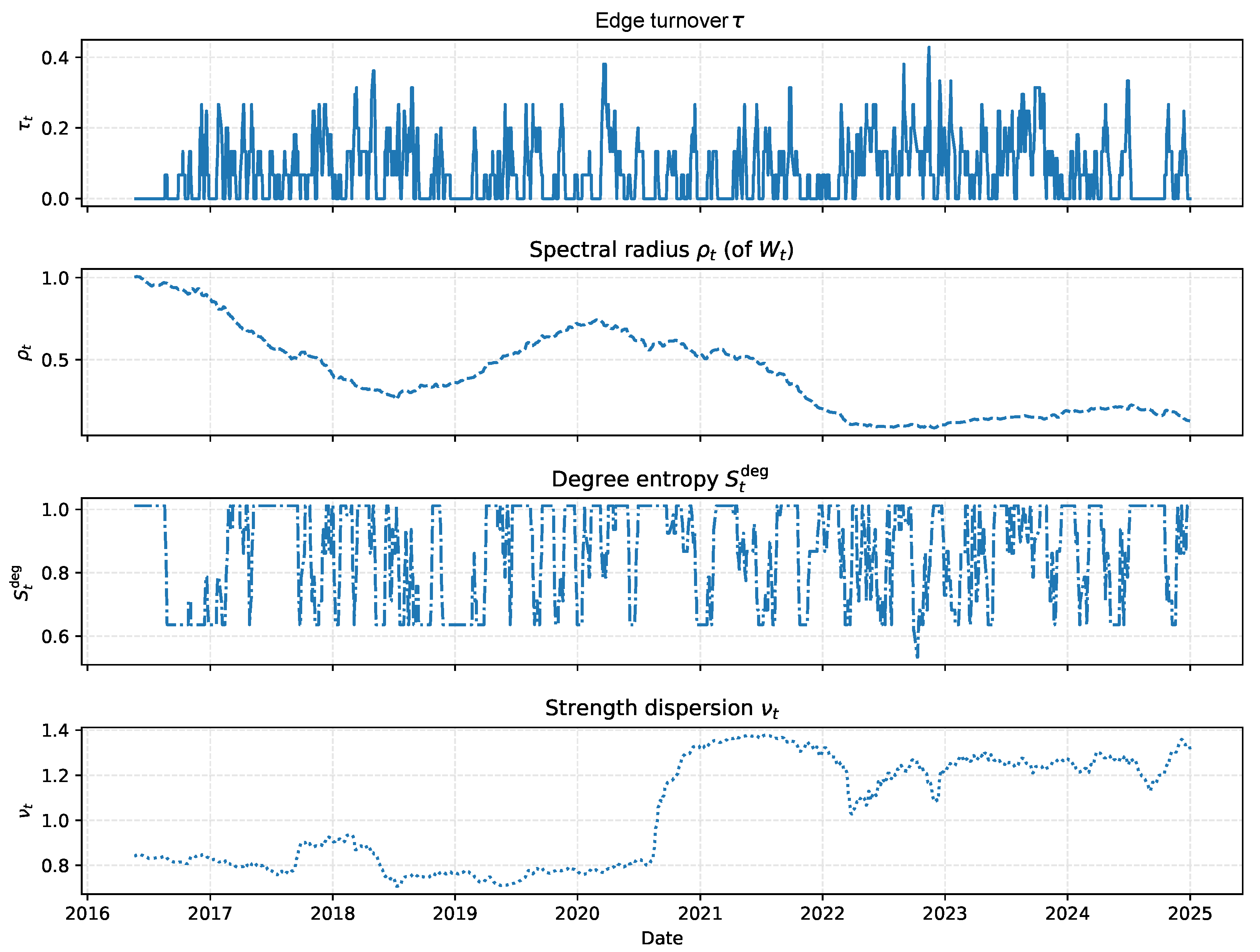
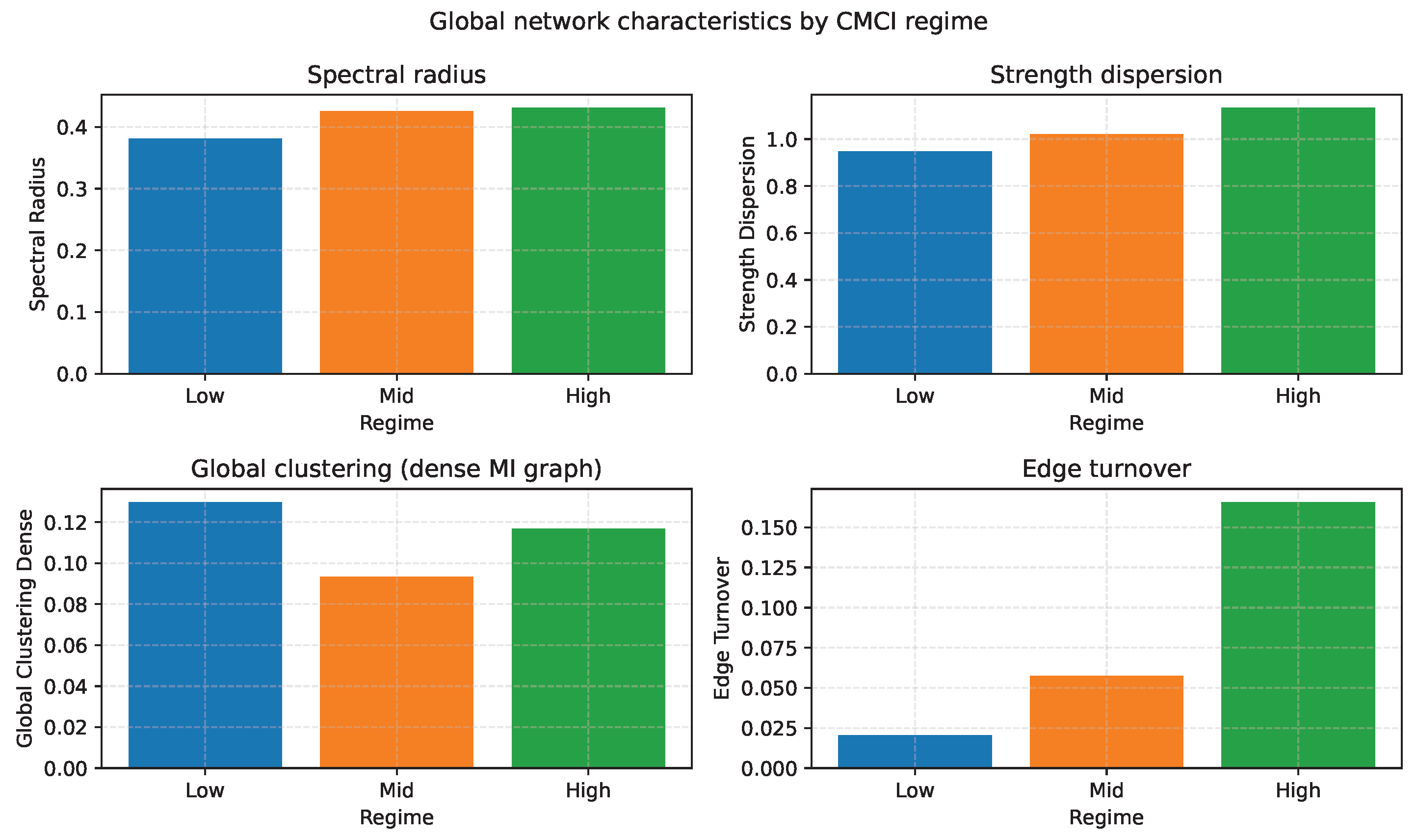
Global clustering and network turbulence. 

Table 9. Global network characteristics by CMCI regime.

Regime	${\mathit{\rho }}_{\mathit{t}}$ (Spectral Radius)	Strength Dispersion	Global Clustering	Edge Turnover	Modularity
Low CMCI	0.381	0.949	0.130	0.020	0.326
Mid CMCI	0.426	1.020	0.093	0.058	0.267
High CMCI	0.431	1.133	0.117	0.166	0.187

summarizes global diagnostics, edge turnover ${\tau }_t$, spectral radius ${\rho }_t$, strength dispersion ${\upsilon }_t$, global clustering ${\mathcal{C}}_t^{\left(\mathrm{glob}\right)}$, and modularity, by CMCI regime. Moving from low to high CMCI, edge turnover rises, indicating faster reallocation of connections; the spectral radius increases, pointing to stronger amplification of shocks along the network; and strength dispersion widens, implying a more unequal distribution of centrality across nodes. At the same time, global clustering ${\mathcal{C}}_t^{\left(\mathrm{glob}\right)}$ tends to be higher in high-CMCI states than in low-CMCI states, suggesting that assets form tighter groups through which shocks can circulate, even as modularity declines and communities become less clearly separated.

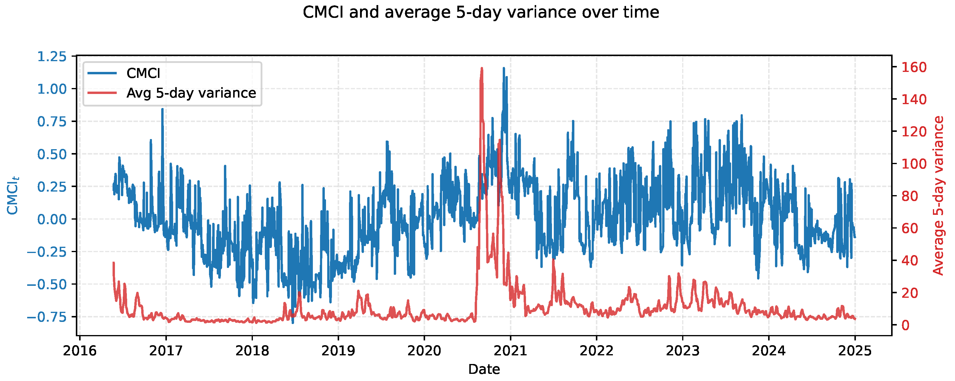
Figure 10 plots the time series of ${\mathrm{CMCI}}_t$ together with standardized global metrics. Peaks in ${\mathrm{CMCI}}_t$ coincide with spikes in spectral radius, strength dispersion, and global clustering, especially around major events such as the 2016 oil-price collapse, the COVID-19 shock, and the subsequent monetary-tightening cycle. The co-movement between CMCI and these network indicators reinforces the interpretation of CMCI as capturing both local chaos in oil and systemic turbulence in cross-asset linkages.

Implications for risk transmission and forecasting. The network evidence indicates that high-CMCI regimes are marked by (i) a more centralized and tightly clustered global equity structure and (ii) stronger, more volatile linkages between energy-sector indices and the broader market. These features offer a structural interpretation of the forecasting results in Section 3.4: when ${\mathrm{CMCI}}_t$ is elevated, shocks originating in oil and energy-related assets are more readily transmitted through the dependence network, increasing the likelihood that they evolve into substantial fluctuations in realized variance.

From a risk-management perspective, the Discussion results imply that ${\mathrm{CMCI}}_t$ is informative not only about the level of volatility but also about the configuration of cross-asset dependencies. In calm regimes, the network is more diffuse and less clustered, so idiosyncratic shocks tend to remain localized. In chaotic regimes, network clustering and spectral radius increase, creating conditions for systemic episodes in which a shock to one or two central nodes can generate widespread turbulence. These structural differences help explain why incorporating ${\mathrm{CMCI}}_t$ and network-based features improves multi-asset variance forecasts and downside-risk measures in our panel framework.

Comparison with existing literature. Our regime-dependent results are consistent with the literature showing that oil–equity dependence and spillovers strengthen under stress and turbulence and that such linkages are nonlinear and state-dependent (Aromi & Clements, 2019; Arouri et al., 2012; Hernandez et al., 2022; Li, 2022; Naifar & Al Dohaiman, 2013). The observed increase in connectivity and centralization during high-CMCI regimes also aligns with network-based evidence that market structures reorganize during turbulent episodes and can concentrate shock transmission channels (Hasse, 2022; Khoojine & Han, 2020; Neveu, 2018; Sioofy Khoojine & Han, 2019; Wu et al., 2022). In contrast to studies that focus on either nonlinear oil-market behavior or interconnectedness in isolation, our contribution is to integrate both channels into a single CMCI state variable that jointly reflects the emergence of instability and the strengthening of propagation mechanisms. Additionally, relative to oil-volatility forecasting approaches based on GARCH-type dynamics and macro-financial predictors (Chen et al., 2022; Hong et al., 2022; Klein & Walther, 2016; Nonejad, 2020; Wei et al., 2010), CMCI contributes a parsimonious state variable that combines nonlinear oil-market complexity with systemic connectedness, helping explain its incremental predictive content in our variance forecasting framework.

5. Conclusions

Financial markets have consistently demonstrated susceptibility to systemic turbulence, and oil and equity markets provide no exception. This study examines such disturbances within a multilayer analytical framework and introduces an indicator designed to provide rapid warning of sudden and severe instability. The short-term prediction of risk has long attracted the attention of researchers and practitioners in both markets. To address this objective, the analysis adopts a three-stage structure consisting of an Oil Complexity Index, a Network Volatility Index, and a final composite indicator. The Oil Complexity Index measures the degree of chaotic behavior in crude-oil markets. It combines multifractal statistics derived from MF-DFA with permutation entropy, approximate entropy and Lyapunov exponents to create an integrated diagnostic tool, which is applied to Brent and WTI time series. The second stage constructs an index that evaluates the relationship between equity and energy markets through a mutual-information network. This network includes several structural components, Edge Turnover, Spectral Radius, Degree Entropy and Strength Dispersion, each with a distinct role in detecting potential instability within the system.

The third stage develops a panel forecasting model that incorporates these indices as explanatory variables and produces predictions for five-day realized variance. The model also includes three macro-financial controls, the USD/CNY exchange rate, the VXX volatility index and the policy interest rate, to capture the influence of broader economic conditions. The empirical results for the oil market indicate that both Brent and WTI exhibit strong multifractality, high entropy and positive Lyapunov exponents. Their price behavior is therefore multiscale, chaotic and sensitive to initial conditions. These characteristics reveal the inherent complexity of oil-price dynamics. The composite Oil Complexity Index rises sharply during periods of stress and market shocks, demonstrating that these episodes coincide with heightened disorder in the structure of oil returns.

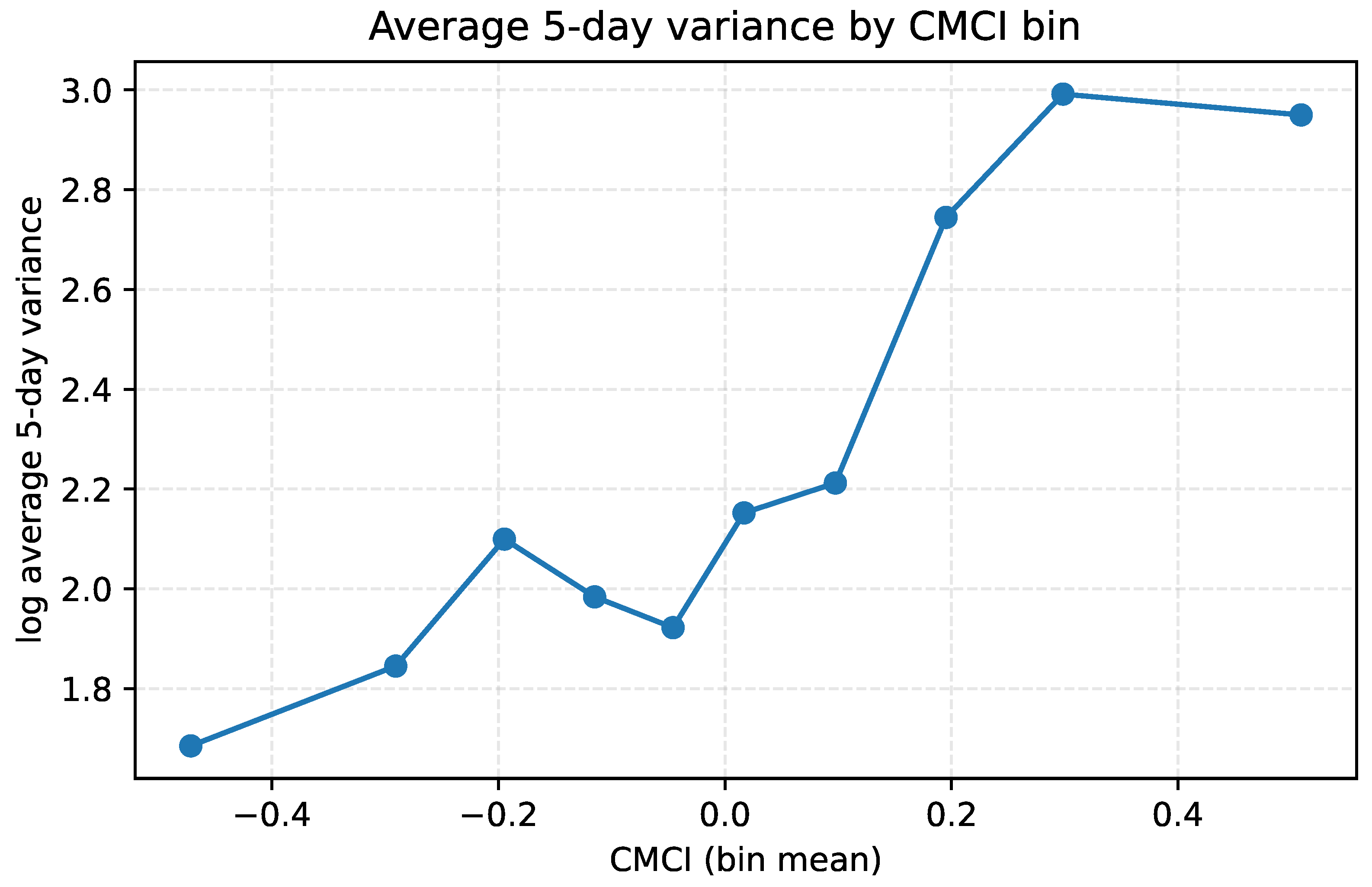
The dependency network displays similarly informative patterns. During turbulent intervals, the network experiences episodic edge turnover, which reflects rapid changes in its connectivity. The spectral radius also increases, indicating greater capacity for shock amplification and transmission. In addition, dependence becomes concentrated in a limited number of influential nodes, creating a more fragile and less resilient structure. Elevated values of the composite index (CMCI) therefore indicate that the market occupies a highly unstable state. During such periods, realized volatility and the VXX index increase simultaneously. The five-day realized variance of equity indices is approximately three times larger in high-CMCI regimes than in low-CMCI regimes, indicating a substantial rise in short-term risk. The network also becomes more clustered and centralized, which causes asset behavior to converge and enables shocks to spread more rapidly across the system.

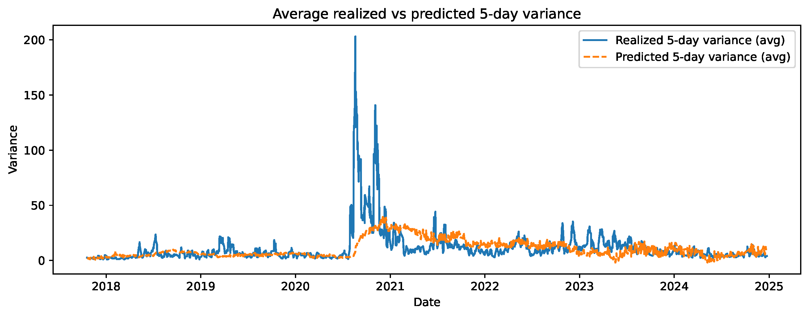
Inclusion of the CMCI, or its two components, within the forecasting model produces a marked improvement in predictive accuracy relative to models that rely only on external variables such as exchange rates, interest rates or VXX. Forecast errors decline significantly, as reflected in measures such as MSE and QLIKE, and the Diebold–Mariano test confirms the statistical significance of these improvements. Conceptually, the CMCI indicates that local complexity in the oil market and turbulence in the equity-market network do not operate in isolation; instead, they strengthen one another. As complexity and volatility intensify in the oil market, the equity-market network becomes more fragile and more concentrated, and this interaction moves the system towards a chaotic state. Methodologically, the CMCI presents a unified framework that integrates measures of complexity and chaos with structural information from networks to create an interpretable state variable suitable for risk modeling. The final stage develops a panel-based forecasting model that uses the two indices. First, the indices are entered jointly as an independent variable, and then the model generates predictions for five-day realized variance. Three macro-financial variables, the USD/CNY exchange rate, the VXX volatility index, and the policy interest rate, are added to control for broader economic conditions.

From an investor perspective, the CMCI can be interpreted as a real-time state variable summarizing the intensity of oil–equity systemic turbulence. Practically, it can be used to (i) identify high-stress regimes in which return predictability deteriorates and downside risk increases, (ii) implement dynamic risk budgeting (e.g., reducing leverage or tightening risk limits when CMCI is elevated), and (iii) trigger cost-aware hedging overlays such as index option protection or volatility exposure. In addition, CMCI can complement conventional stress indicators (e.g., VIX and realized volatility) because it embeds information on nonlinear complexity and network spillovers, and can be included as an explanatory variable in forecasting and risk models (e.g., VaR/ES or regime-switching allocation rules).

Potential limitations should be noted. The CMCI is constructed from rolling-window estimates and therefore depends on several design choices (e.g., window length, MF–DFA settings, embedding/entropy/Lyapunov parameters, the mutual-information estimator and its tuning, network sparsification rules, regime thresholds, and the CMCI weights). These choices can introduce estimation noise and a detection lag around turning points, and CMCI should be interpreted as a descriptive state variable rather than a causal measure or a stand-alone trading rule. To mitigate these concerns, we conduct extensive robustness checks across the above choices (including alternative sparsifiers and a PCA-based weighting scheme) and find that CMCI dynamics, regime patterns, and the main forecasting conclusions are not sensitive to reasonable alternative specifications.

The CMCI advances systemic-risk forecasting by combining oil-market nonlinear complexity with time-varying network turbulence into a single, interpretable state variable. Because it captures both irregular local dynamics and strengthened spillover channels, CMCI provides incremental information for identifying high-stress regimes and improving short-horizon risk forecasts beyond conventional volatility proxies.

Future work may extend the CMCI to other asset classes such as bonds, cryptocurrencies and smaller industry sectors, or to higher-frequency intraday data. The use of regime-switching nonlinear models with the CMCI as a state variable may also yield a more accurate description of the dynamics of volatility. Further incorporation of sequential or multilayer networks could allow the analysis of even more complex risk structures.