Mining Frequent Sequences with Time Constraints from High-Frequency Data

Abstract

Investing in the stock market has always been an exciting topic for people. Many specialists have tried to develop tools to predict future stock prices in order to make high profits and avoid big losses. However, predicting prices based on the dynamic characteristics of stocks seems to be a non-trivial problem. In practice, the predictive models are not expected to provide the most accurate forecasts of stock prices, but to highlight changes and discrepancies between the predicted and observed values, to warn against threats, and to inform users about upcoming opportunities. In this paper, we discuss the use of frequent sequences as well as association rules in WIG20 stock price prediction. Specifically, our study used two methods to approach the problem: correlation analysis based on the Pearson correlation coefficient and frequent sequence mining with temporal constraints. In total, 43 association rules were discovered, characterized by relatively high confidence and lift. Moreover, the most effective rules were those that described the same type of trend for both companies, i.e., rise ⇒ rise, or fall ⇒ fall. However, rules that showed the opposite trend, namely fall ⇒ rise or rise ⇒ fall, were rare.

1. Introduction

For many people, investing in the stock market has always been an exciting activity. For a long time, specialists have been designing systems that aim to help investors achieve high returns and also reduce the risk of losses. Such decision support systems are expected to quickly detect discrepancies between predicted and observed values, while warning of risks or informing of upcoming profit opportunities. However, due to the dynamic nature of stock prices, this task seems to be a non-trivial problem.

Associations are defined as relations between companies, for which there are common patterns of reaction to market changes. Assuming that, as in nature, phenomena are subject to the law of action and reaction, this law also applies to the stock market, where a change in the price of one company affects the other. In this line of thinking, in this paper we address the problem of mining frequent sequence mining with time constraints from high-frequency data. Also, it is important to note that stock prices often reflect long-term trends and economic conditions. While returns capture short-term fluctuations, price correlations can be useful for analyzing structural relationships between companies over extended periods.

The rest of this paper is structured as follows. Section 2 provides the theoretical background and motivation. Section 3 gives an overview on the methodology applied. Section 4 introduces the results obtained from the study conducted, followed by the discussion in Section 5. Eventually, Section 6 outlines the final conclusions.

2. Theoretical Background

Even though the stock market is considered unpredictable and erratic, it has already been proved that artificial intelligence (AI) and machine learning (ML) strategies can be applied for market behavior prediction based on patterns predicted from historical pricing data (Fiol-Roig et al., 2010). Recent studies have further emphasized this trend, showing that AI-driven approaches can capture complex market dependencies and improve forecasting accuracy (Jain & Vanzara, 2023). It has also been shown that combining various input sources, e.g., information hidden in the market news with stock prices or social media sentiment analysis, can lead to even better accuracy (X. Li et al., 2011; Mehta et al., 2021).

So far, various methods have already been proposed for stock market data mining, including statistical methods (Kannan et al., 2010) as well as some conventional ML techniques, e.g., decision trees, support vector machines, Bayesian, K-nearest neighbors, K-means, Expectation–Maximization algorithm, ensemble learning (Liu et al., 2021), and neural networks (Safer, 2003). More recently, due to the rapid progress in deep learning (DL) techniques, multiple studies have shifted towards such solutions due to their potential to achieve more accurate predictions and generalize better to previously unknown data inputs (Kwaśniewska et al., 2017). Research on deep learning models, such as LSTM and GRU, has demonstrated their strong predictive capability for economic trends and stock market prices (Chang et al., 2024). In the study performed by Bhandari et al. (2022), a single-layer long short-term memory (LSTM) model was used to predict the next-day price of the S&P 500 index, leading to the root mean squared error (RMSE) being around 40.5, proving its reliability in predicting closing prices.

On the other hand, Staffini (2022) argued that LSTMs are not the best topologies for market analysis and proposed a stock price forecasting method based on a deep convolutional generative adversarial network to further improve prediction accuracy compared to LSTMs. In a different work, more emphasis was put on the data cleaning and pre-processing step, showing that LSTM can still achieve superior performance if data are carefully selected and prepared using, e.g., dimensionality reduction with principal component analysis (PCA) (Shen & Shafiq, 2020). A recent study also explored the application of spatiotemporal deep learning, introducing the Spacetimeformer model, which enhances forecasting by capturing both spatial and temporal dependencies among stocks (Y.-C. Li et al., 2023). Other DL methods have also been already applied for similar applications, e.g., stock price prediction using historical data and multilayer perceptron (MLP), recurrent neural networks (RNNs), or convolutional neural networks (CNNs) separately (Hiransha et al., 2018), as well as hybrid combinations of multiple topologies (Kanwal et al., 2022).

On the other hand, even though ML can address some limitations of statistical methods (Bzdok et al., 2018), most of the methods proposed for stock market analytics are trained in a supervised setting, allowing for superior classification performance (Subasi et al., 2021) but only for strictly defined categories, such as price movements: falling, rising, neutral, trend continuation, and trend-reversal patterns (Strader et al., 2020). This approach fails to discover new patterns (Shah et al., 2019), which is frequently crucial for investment planning and other decision-making processes (Wasserbacher & Spindler, 2021). A comprehensive review of AI-based stock market forecasting has highlighted the importance of hybrid models and data pre-processing in improving predictive accuracy (Chopra & Sharma, 2021).

In the view of the foregoing, this study focuses on mining frequent sequences using the Apriori algorithm, eliminating the need for labeled samples. In addition, the proposed algorithm is modified to preserve the order of items, ensuring that the real behavior of the stock market is maintained, which may influence produced outcomes and thus also the actions taken based on the performed analysis.

3. Methodology

Our study was quantitative in nature Anderson et al. (2018), which means carrying out research to make use of factual data to discover previously unknown and non-trivial knowledge. To be more precise, it falls into the scope of the data mining research stream of time series analysis Bederson and Shneiderman (2003). An iterative and interactive research design was used consisting of a descriptive analysis (Glass et al., 2008) and inductive reasoning (Klauer & Phye, 2008). Note that, while the former aims at decomposing the series into elementary components, the latter involves the searching for frequent patterns (relationships) from a set of the observations. In addition, for the purpose of this study, we designed and implemented a modular software package to perform simulations.

In modern software engineering, modularity of information systems enable the use of individual components of the system independently (Sullivan et al., 2001), arguing that each particular module should be easy to understand, test, modify, replace, or erase in isolation without affecting the rest of the system. Moreover, such architecture design let already-made components to be reused in other systems.

In our study, we adopted the concept of the modularity in our software design. Modularity was also used when designing a solution for the problem. The proposed system, thanks to its modular structure, allows for the easy replacement of one of the modules in order to introduce a new component. The new component can be related to data processing, the algorithm itself, or visualization of the results.

3.1. Input Data

In our study, we used the tick dataset from the Warsaw Stock Exchange (WSE), covering the sell/buy transactions from 1 August 2020 to 31 January 2021, including twenty largest companies Warsaw Stock Index (WIG20). As of 15 September 2020, the WSE listed shares of 436 companies (including 48 foreign entities). On average, in total 250 thousand transactions are performed daily by both institutional and individual investors.

For the purpose of the analysis, a unique transaction was limited to the four attributes, namely (i) name, (ii) date and time, (iii) price (with two decimals), and (iv) volume. Note that the volume is the daily number of stock shares that has changed the owner. A sample of the raw data is given in

Table 1. Selected three transactions for PKN Orlen during the day on 14 August 2020.

Name	Date and Time	Price	Volume
PKNORLEN	14 August 2020 09:00:00.464644	55.86	9
PKNORLEN	14 August 2020 09:00:00.464654	55.86	14
PKNORLEN	14 August 2020 09:00:00.900500	55.86	3

below.

A tick dataset is characterized by high frequency and irregularity. While the former means that any analysis requires high processing capacity, then the latter concerns the issue of different amounts of recorded transactions of particular stocks, regarding a fixed period of time.

The rate of return (RoR) is a measure of the change in the value of an investment over a given period of time (de La Grandville, 1998), which can be positive, negative, or zero. It shows the profitability of an investment and is calculated as follows (Equation (1)):

$$RoR={\displaystyle \frac{V_c-V_i}{V_i}}$$

(1)

where V_c—current value, V_i—initial value.

3.2. Methods

In the first run, we used Pearson correlation coefficient (r) in order to determine the degree of correlation between stock prices of two stocks. To calculate this value, the following formula was used:

$$r={\displaystyle \frac{{\sum }_{i=1}^n(x_i-\overline{x})(y_i-\overline{y})}{\sqrt{{\sum }_{i=1}^n{(x_i-\overline{x})}^2}\sqrt{{\sum }_{i=1}^n{(y_i-\overline{y})}^2}}}$$

(2)

where x_i—values of the x-variable in a sample, $\overline{x}$—mean of the values of the x-variable, y_i—values of the y-variable in a sample, $\overline{y}$—mean of the values of the y-variable, n—sample size.

In the second run, we used the modification of the Apriori algorithm (Agrawal et al., 1993), which is a well-known and widely used method for mining frequent itemsets. However, one should be aware of its major assumption, which violates the order of elements by requiring as an input transactions’ items sorted in ascending order. In practice, this means that two transactions t₁ = {i₁, i₂, i₃} and t₂ = {i₂, i₃, i₁}, after the sorting operation, will be identical.

Therefore, appropriate modifications must be made to maintain the order of the elements. In other words, both the order and the length of a sequence must be satisfied in the support calculation. Note that such an order assumption requires modifications to the Apriori algorithm that increase the computational cost of the algorithm by increasing the number of candidates. However, preliminary experiments have shown that the modifications do not significantly degrade the performance of the algorithm since the number of possible cases is limited to two, involving a rise or fall in the stock price.

Considering the problem of frequent itemsets mining, let D = {t₁, t₂, …, t_m} be a set of m transactions called the database, and let I = {i₁, i₂, …, i_n} be a set of n binary attributes called items. The basic concept is the support (sup) which refers to the frequency of occurrence of each subset in the database D. It is determined by the ratio of the number of transactions in which a subset occurs to the number of total transactions. The minimum support is defined as the minimum number of occurrences of the item (itemset) in the database, and if the item (itemset) fulfills this condition is called frequent item (itemset).

An association rule (R) is defined as an implication of the form X ⇒ Y, where X, Y ⊆ I and X ∩ Y = ∅. While a rule has the same support (Equation (3)) as the frequent itemset which it is implied from, there are two other basic measures, namely confidence (Equation (4)) and lift (Equation (5)), which describe its significance and importance, respectively.

$$sup(X\Rightarrow Y)={\displaystyle \frac{sup(X,Y)}{\mathit{m}}}$$

(3)

$$conf(X\Rightarrow Y)={\displaystyle \frac{sup(X,Y)}{sup\left(X\right)}}$$

(4)

$$lift(X\Rightarrow Y)={\displaystyle \frac{sup(X\Rightarrow Y)}{sup\left(X\right)\ast sup\left(Y\right)}}$$

(5)

It is assumed that only the minimum support is required from a user to be provided, as the input parameter of the Apriori algorithm. However, in order to reduce the number of association rules, in our method, termed as the s-Apriori, the minimum thresholds for both confidence and lift are also required to be given.

4. Results

Determining the correlation between companies is an intermediate element, the purpose of which is to determine the degree of correlation between the stock prices of two individual listed companies. To determine this value, Pearson’s linear correlation coefficient was used (Equation (2)).

The correlation was determined for all combinations of WIG20 index companies (the total number of combinations is 190). In addition, in order to perform an in-depth analysis, the correlation was determined for different time intervals. The entire process of determining the correlation between companies was as follows:

• Determine all possible combinations between companies.
• Determining the time intervals given in minutes.
• Sampling the data according to the set interval.
• Calculating the rate of return for each company. Return rates were calculated between successive prices sampled according to the set interval according to Formula (1).

Note that, for clarity, the strongest positive correlation for each pair is always highlighted when they are not all equal for all time intervals.

In the current study, the following intervals were used: 5, 10, 15, 20, 25, 30, 35, 40, 45, 50, 55, 60, 65, 70, 75, 80, 85, 90, 95, 100, 125, 150, 175, 200, 225, 250, 375, 500, 750, 1000, 1250, 1500. The selected results are shown in

Table 2. Values for daily correlations for returns between the following companies Allegro S.A.-Asseco Polska S.A., Asseco Polska S.A.-Mercatron Medical S.A., Cyfrowy Polsat S.A.-Orange Polska S.A., CCC S.A.-Bank PEKAO S.A., Mercatron Medical S.A.-PKN Orlen S.A., Lotos S.A.-PKN Orlen S.A., Bank PEKAO S.A.-PKO BP S.A. The data covered the five-month period from 1 August 2020 to 31 December 2020.

Int. (min)	ALE-ACP	ACP-MRC	CPS-OPL	CCC-PEO	MER-PKN	LTS-PKN	PEO-PKO
5	0.03	0.03	0.21	0.23	−0.01	0.50	0.57
10	0.05	0.04	0.23	0.32	0.01	0.60	0.65
15	0.07	0.04	0.32	0.31	0.00	0.64	0.69
20	0.05	0.03	0.31	0.37	−0.01	0.66	0.70
25	0.10	0.07	0.38	0.37	−0.04	0.71	0.73
30	0.09	0.06	0.38	0.35	0.00	0.68	0.75
35	0.08	0.10	0.42	0.36	−0.07	0.72	0.75
40	0.13	0.07	0.43	0.45	−0.08	0.72	0.78
45	0.14	0.11	0.44	0.36	−0.04	0.70	0.76
50	0.17	0.07	0.43	0.42	−0.08	0.73	0.79
60	0.22	0.15	0.39	0.35	−0.03	0.73	0.77
1000	0.20	−0.02	0.60	0.48	−0.31	0.82	0.94
1250	−0.09	−0.01	0.53	0.63	−0.28	0.77	0.97
1500	0.00	0.00	0.49	0.52	−0.21	0.81	0.93

.

Table 2 shows the values of the correlation coefficient for selected pairs of companies in the WIG20 index. Among the pairs presented, we can note the combinations for which there is a high correlation, for example: [Grupa Lotos and PKN Orlean] and [Bank PEKAO and Bank PKO BP]. It is worth noting that, in the case of these two pairs, both companies are from the same economic sector, which may be the reason for the high correlation between them.

On the other hand, between the pairs [Allegro and Asseco Polska], [Asseco Polska and Mercatorn Medical], and [Mercatorn Medical and PKN Orlen], the value of correlation oscillates around zero. This means that the share values of the paired companies are not correlated with each other. It is also worth noting that, as the interval increases, the value of the correlation coefficient also increases. This phenomenon can be observed in the following pairs: [Cyfrowy Polsat-Orange Polska], [CCC and PEKAO ], [Lotos and PKN Orlen], and [PEKAO and PKO BP]. Such correlations are not surprising due to the fact that the correlations were calculated on the basis of returns. For the 5 min interval, the price changes are small due to the short observation time. As the interval increases, the chance of capturing price changes increases, which makes it possible to determine the behavioral characteristics of companies over time.

Within the framework of this study, the analysis was carried out for the relationship between companies in the daily window. Due to this fact, the maximum interval length was set at 60 min. In the case of the WSE, the trading session lasts eight hours, so eight samples obtained during the day are the minimum number to observe the relationship between companies. In Table 2, intervals less than or equal to 60 min are highlighted with a bold line in order to distinguish the intervals that will be considered in the following section.

Table 3. Values for the correlation intraday by share price between the following pairs: [Allegro and Asseco Polska], [Asseco Polska and Mercatorn Medical], [Cyfrowy Polsat and Orange Polska], [CCC and PEKAO], [Mercatorn Medical and PKN Orlen], [Lotos and PKN Orlen], and [PEKAO and PKO BP]. The data covered a 5-month period from 1 August 2020 to 31 December 2020.

Int. (min)	5	10	15	20	30	40	45	50	60
PKOBP-SANPL	0.97	0.97	0.97	0.97	0.97	0.97	0.97	0.97	0.97
PEKAO-PKOBP	0.94	0.94	0.94	0.94	0.94	0.94	0.94	0.94	0.94
PEKAO-PKNORLEN	0.92	0.92	0.92	0.92	0.92	0.92	0.92	0.92	0.92
MERCATOR-PZU	0.72	0.72	0.72	0.72	0.72	0.72	0.72	0.72	0.72
LOTOS-ORANGEPL	0.56	0.56	0.56	0.56	0.56	0.57	0.57	0.56	0.56
ALLEGRO-DINOPL	0.14	0.14	0.14	0.14	0.14	0.14	0.14	0.14	0.14
ASSECOPOL-CCC	0.04	0.04	0.04	0.04	0.04	0.04	0.04	0.04	0.04
CDPROJEKT-KGHM	0.54	0.54	0.54	0.54	0.54	0.54	0.53	0.54	0.54
JSW-PGE	0.16	0.16	0.16	0.16	0.16	0.16	0.15	0.16	0.15
JSW-TAURONPE	0.07	0.07	0.08	0.08	0.07	0.07	0.07	0.08	0.07
PGE-TAURONPE	0.86	0.86	0.86	0.86	0.86	0.86	0.87	0.86	0.86

and

Table 4. Values for the correlation intraday of interest rates between the following pairs: [PKO BP and Santander], [Bank PEKAO and PKO BP], [Bank PEKAO and PKN Orlen], [Mercatron Medical and PZU ], [Lotos and Orange], [Allegro and Dino], [Asseco and CCC], [CD Projekt and KGHM], [JSW and PGE], [JSW and Tauron], and [PGE and Tauron]. The data covered a 5-month period from 1 August 2020 to 31 December 2020.

Int. (min)	5	10	15	20	30	40	45	50	60
PKOBP-SANPL	0.40	0.47	0.52	0.53	0.58	0.63	0.60	0.65	0.61
PEKAO-PKOBP	0.57	0.65	0.69	0.70	0.75	0.78	0.76	0.79	0.77
PEKAO-PKNORLEN	0.32	0.38	0.40	0.42	0.44	0.51	0.45	0.44	0.46
MERCATOR-PZU	0.01	0.01	0.02	0.00	0.03	0.05	0.02	0.03	0.03
LOTOS-ORANGEPL	0.12	0.14	0.16	0.16	0.16	0.21	0.17	0.17	0.18
ALLEGRO-DINOPL	0.00	0.01	0.01	0.00	0.04	0.03	0.04	0.03	0.06
ASSECOPOL-CCC	0.06	0.07	0.08	0.06	0.11	0.11	0.13	0.11	0.13
CDPROJEKT-KGHM	0.07	0.02	0.04	0.02	0.01	0.07	0.04	0.05	0.04
JSW-PGE	0.20	0.24	0.26	0.32	0.38	0.38	0.39	0.36	0.43
JSW-TAURONPE	0.21	0.27	0.30	0.32	0.40	0.40	0.40	0.38	0.44
PGE-TAURONPE	0.48	0.59	0.65	0.68	0.72	0.74	0.71	0.73	0.80

present the results for the correlation coefficient for selected pairs of companies in the WIG20 index. The tables show the correlation values for the following intervals: 5-, 10-, 15-, 20-, 30-, 40-, 45-, 50-, and 60-min intervals. Table 3 contains correlations calculated using prices, while Table 4 shows correlations calculated using returns. In order to correctly interpret the results of the correlation coefficient, scatter plots must be generated for the variables that are subject to correlation analysis. 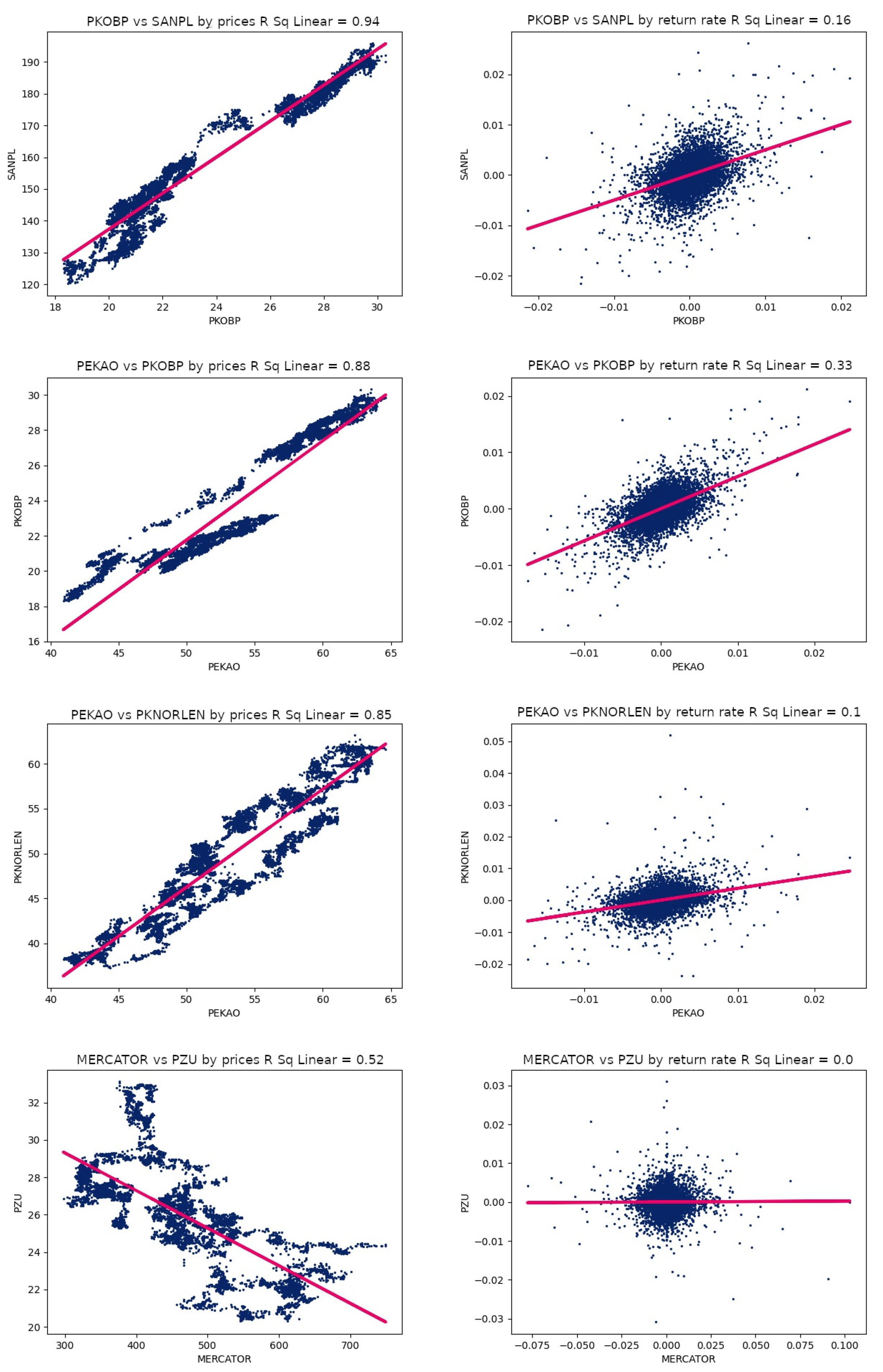Figure 1 shows the scatter plots for the following pairs: [PKO BP and Santander], [Bank PEKAO and PKO BP], [PEKAO and PKN Orlen], and [Mercatorn Medical and PZU].

The scatter charts based on stock prices will be analyzed first. All the four pairs of companies mentioned are characterized by a high correlation coefficient calculated on the basis of stock prices. In addition, on the charts themselves we can observe a linear relationship of the data—the points are spaced in a fairly systematic way along a straight line. The most accurate possible regression line has also been plotted on the charts, which makes it easier to assess the correlation. In the first three charts, we have a positive correlation, as the slope of the regression line is positive. On the other hand, in the last chart, the pair Mercatorn Medical S.A. and PZU S.A. are negatively correlated.

Having determined the direction of the correlation, the next step is to determine the strength of the correlation. For this purpose, two related coefficients will be used: the Pearson correlation coefficient and the coefficient of determination. From Table 3, you can read the results for Pearson’s correlation coefficient, which for the pair PKO BP and Santander is $0.97$.

This correlation can be classified as extremely strong. The value of the coefficient of determination is included in the title of the chart of the statement under discussion and is $0.94$. This value is often presented in percentage notation and indicates the degree to which the regression line approximates the points determined by pairs of values of two variables. When analyzed in terms of the correlation between two companies, the coefficient of determination represents the percentage of the total price volatility of one company that can be explained by a linear relationship between the companies.

For the pair PKO BP and Santander, the coefficient is $0.94$, which means that $94\%$ of the total price volatility of PKO BP can be explained by a linear relationship between PKO BP and Santander. Exactly the same statement can be made for Santander. In the case of the last pair, Mercatron Medical and PZU, the coefficient of determination was $52\%$, while the Pearson correlation coefficient is $-0,72$, demonstrating a moderately strong correlation.

In addition to the scatter charts made on the basis of stock prices, charts made on the basis of the rate of return were also presented. The first difference that can be seen between the pairs of charts is the different scatter characteristics of the data. In the case of charts based on stock prices, a clear linear relationship can be seen, while in charts based on rates of return, the points are concentrated at a single point, forming oval shapes. Correlations between pairs of companies calculated on the basis of relative price changes are much weaker than in the case of underlying stock prices.

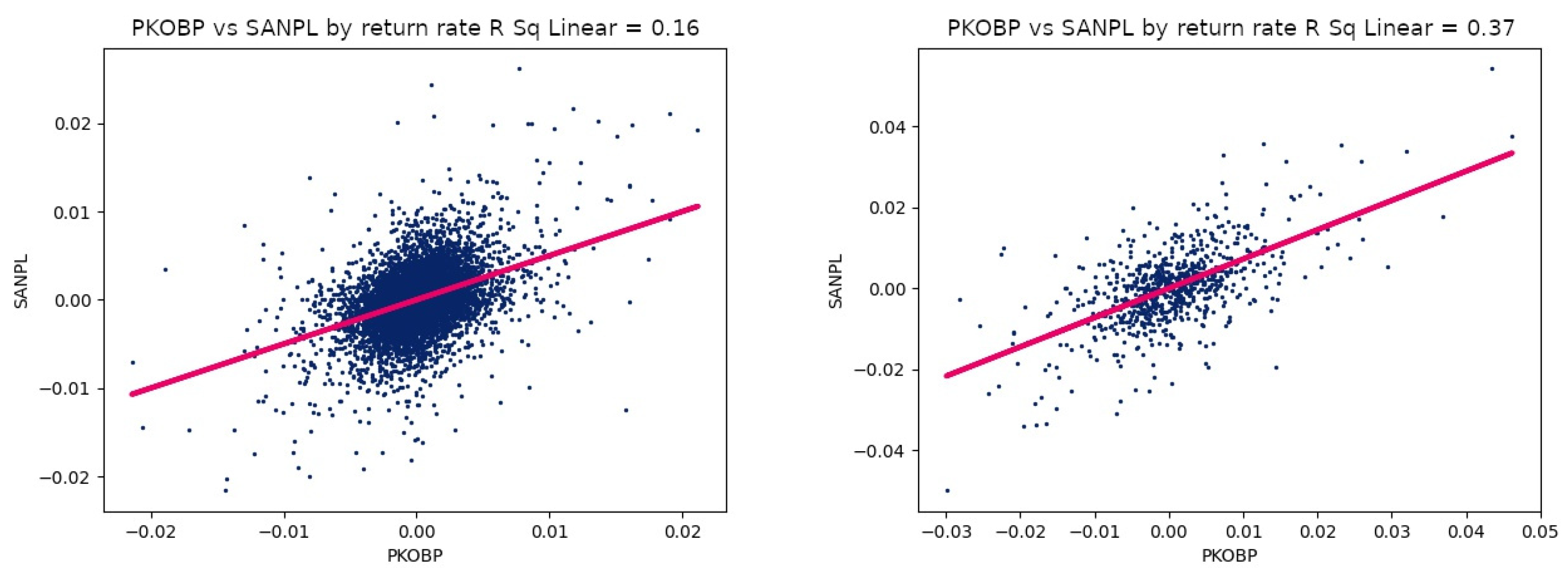
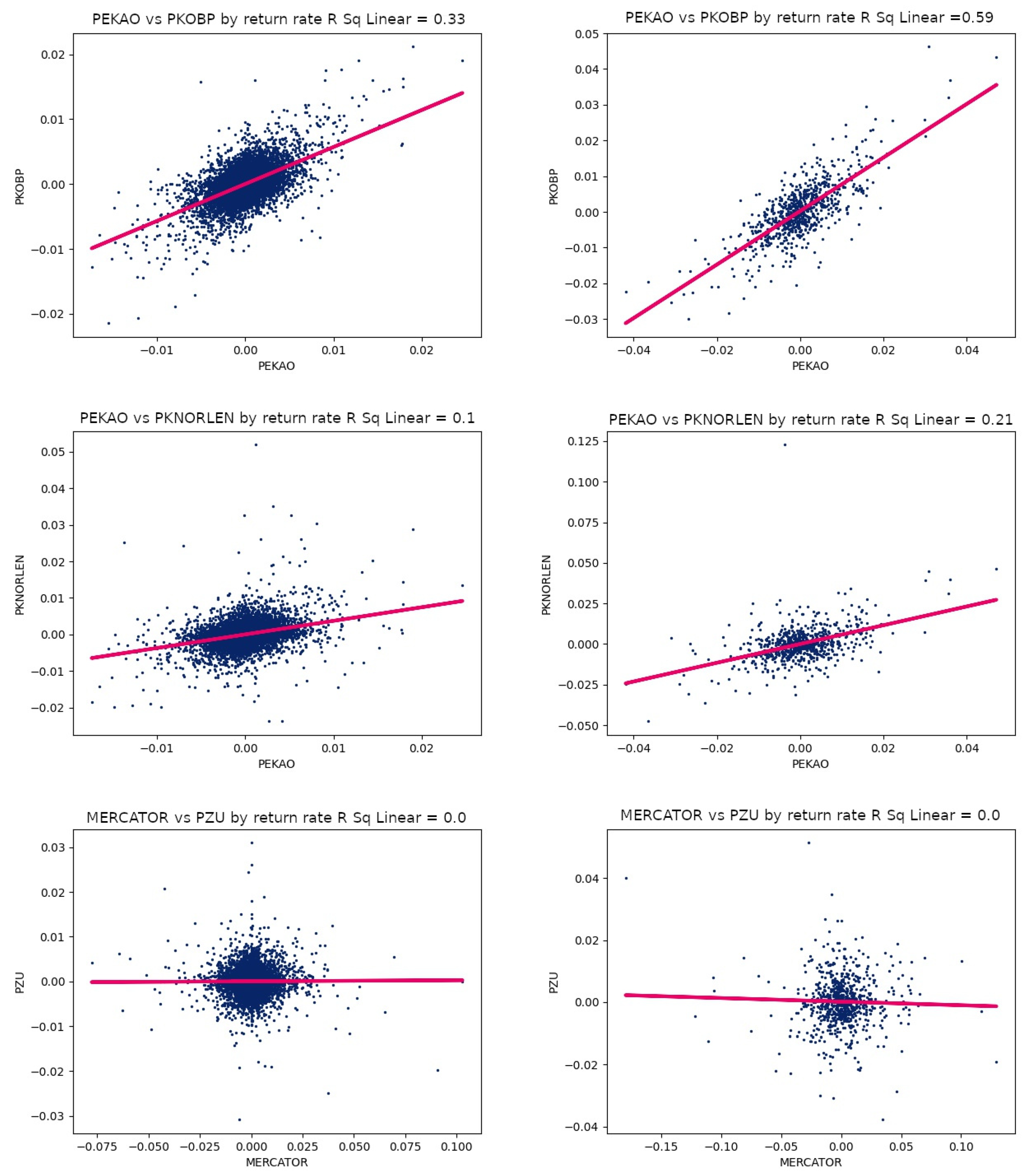
It should be noted that the charts in question are based on data obtained for the 5 min interval. For small intervals, the percentage price changes are close to zero. In the short term, it is difficult to observe large “price jumps”. Comparing the results for individual pairs of companies in Table 3, one can conclude that the interval up of to 60 mins does not affect the value of correlation. A completely different situation is in the case of correlations based on percentage price changes in Table 4. In this case, the length of the interval has a strong influence on the value of the correlation. The following relationship can be observed: the longer the observation interval, the stronger the correlation. Of course, there are minor deviations from this rule, but you can see a strong effect of the length of the interval on the strength of the correlation. For comparison, scatter plots for a 60-min interval are shown in Figure 2.

With small intervals, it is undoubtedly difficult to observe major trends, which are the basis for determining the correlation between two companies. During a trend, there may be short spikes or dips in the price, which have little effect on the main movement of the stock. In the case of the 5 min interval, there is a frequent sampling of stock prices. With such a high frequency, it is possible to register minor fluctuations, which can introduce unnecessary noise that disturbs the analysis of the main trend.

The results obtained using the s-Apriori algorithm are consistent with the results that were obtained for the correlation coefficient. The strongest rules were detected for the following pairs: [PEKAO and PKO BP], [PKO BP and PEKAO S.A.], [PKN Orlen and Lotos], [Lotos and PKN Orlen], [Tauron and PGE], [PGE and Tauron], [PZU and LOTOS], [PEKAO and LOTOS], [PZU and Orlen], [PZU and PKO BP], [PKO BP and Lotos], [PKO BP and Orlen], and [PEKAO and Orlen]. These details are presented in

Table 5. Discovered association rules with corresponding Pearson correlation coefficient for the 60 min interval. The dataset covers the time period from 1 August 2020 to 31 December 2020.

Pair	Rule	Confidence	Lift	Correlation
PEKAO-PKOBP	D⇒D	0.71	1.67	0.77
	U⇒U	0.74	1.70
PKOBP-PEKAO	D⇒D	0.72	1.67	0.77
	U⇒U	0.71	1.70
PKNORLEN-LOTOS	D⇒D	0.72	1.42	0.73
	U⇒U	0.67	1.71
LOTOS-PKNORLEN	D⇒D	0.70	1.42	0.73
	U⇒U	0.63	1.71
TAURONPE-PGE	D⇒D	0.70	1.46	0.80
	U⇒U	0.66	1.57
PGE-TAURONPE	D→D	0.66	1.46	0.80
	U⇒U	0.68	1.57
PZU-LOTOS	D⇒D	0.68	1.35	0.45
	U⇒U	0.58	1.48
PEKAO-LOTOS	D⇒D	0.67	1.33	0.48
	U⇒U	0.53	1.34
PZU-PKNORLEN	D=>D	0.66	1.34	0.45
	U⇒U	0.57	1.56
PZU-PKOBP	D⇒D	0.60	1.41	0.53
	U⇒U	0.65	1.49
PKOBP-LOTOS	D⇒D	0.65	1.29	0.48
	U⇒U	0.52	1.33
PKOBP-PKNORLEN	D⇒D	0.64	1.31	0.45
	U⇒U	0.53	1.44
PEKAO-PKNORLEN	D⇒D	0.64	1.31	0.46
	U⇒U	0.54	1.46

. It is worth noting that, when determining relationships using the s-Apriori algorithm, it is important to maintain the order. In the case of the following rules: $A\left(fall\right)\Rightarrow B\left(fall\right)$ and $B\left(fall\right)\Rightarrow A\left(fall\right)$, both rules may be true, but their confidence and lift may be different. Therefore, two rule variants are included in the results table.

In Table 5, one can observe the consistency in the results of the s-Apriori algorithm and the correlation coefficient. The presented pairs are characterized by strong rules and a high value of the correlation coefficient. In the case of the s-Apriori algorithm, we have a distinction due to the type of rule, so it is possible to determine for which trends there is the strongest relationship. In the case of the companies included in the WIG20, by far the most common rule is the $A\left(fall\right)\Rightarrow B\left(fall\right)$ which has the highest confidence and lift. This is quite often related to the situation in which a decline in the stock price of one company entails more companies. In contrast, in the case of increases, the trend is not so strong that it affects related companies every time.

5. Discussion

The problem of finding relationships between listed companies can be solved using both the Pearson correlation coefficient and frequent sequence mining. Previous studies have mainly focused on finding relations between companies in the long-term context. In this paper, it is proved that the study of short-term periods also gives promising results.

Undoubtedly, the advantage of the frequent sequence mining method is the possibility of detecting non-linear relationships. This is undoubtedly a great advantage over the method based on Pearson correlation coefficient, which is designed only for linear relationships.

In addition, the frequent sequence mining method brings additional information to facilitate the analysis of stock market changes such as the type of rules and the values of the metrics confidence and lift achieved for them. The s-Apriori algorithm effectively discovered the rules with high performance levels, so that the analysis of market changes can be based on the logic defined by the discovered rules.

The rules that had the highest effectiveness during the study were those that described the same type of trend for both companies, e.g., ($rise\Rightarrow rise$) or ($fall\Rightarrow fall$). Rules with opposite trends, e.g., ($fall\Rightarrow rise$) or ($rise\Rightarrow fall$), appeared rarely. Few occurrences of a steady trend were also recorded, so sequences with a steady trend often did not qualify as frequent sequences and consequently for rule construction.

Strong correlations between companies could be observed for companies from the same economic sector, such as banking. The ($fall\Rightarrow fall$) rule for the juxtaposition of banks PKO BP S.A. and Bank PEKAO S.A. obtained a confidence of 0.72 and a growth of 1.62. Similarly high results were achieved for companies in the fuel sector, e.g., for the combination of Lotos S.A. and PKN Orlen S.A. the ($rise\Rightarrow rise$) rule obtained values of 0.63 and 1.71 for confidence and lift, respectively. High results were also achieved for companies from different economic sectors: PKO BP S.A. and and PZU S.A. (both ($fall\Rightarrow fall$) and ($rise\Rightarrow rise$)) rules reached values above 0.6 for confidence and lift; similarly, for the stocks of Bank PEKAO S.A. and LOTOS S.A. ($fall\Rightarrow fall$), the rule reached values above 0.6 for confidence and lift.

6. Conclusions

The method of exploring frequent sequences is an effective tool for determining the degree of portfolio diversification, but also for tracking disturbing changes in the market that may negatively affect an investor’s portfolio. Regardless of the results obtained, however, it is worth supporting the results with additional information about the correlations between companies. This type of information can strengthen the rules and can help explain the presence of strong intercompany relationships.

Another important issue is the validity period of the rules. Rules are not permanent, so you should perform fairly frequent updates on the updated data. When studying daily trends, the regularity of performing the analysis is more important than the amount of historical data. Data from a period of 3 to 4 months is sufficient to determine the relationship between companies. In case of analysis of long-term relations; for example, quarterly or yearly, it is necessary to provide large amount of data with prices at the beginning and end of the day.

The frequent sequence mining method is a promising technique that has proven to be an effective tool to solve the problem posed. It would also be an interesting concept to try to tackle the problem using other machine learning methods such as artificial neural networks. Of particular interest may be recurrent neural networks, whose design is adapted to sequential data. Belonging to the family of recurrent neural networks, the long short-term memory (LSTM) networks, which have an internal memory, may prove to be an interesting direction to further investigate the problem of inter-company relationships.