Active Fault-Tolerant Control for Quadrotor UAV against Sensor Fault Diagnosed by the Auto Sequential Random Forest

Abstract

Active disturbance rejection control (ADRC) is a model-independent method widely used in passive fault-tolerant control of the quadrotor unmanned aerial vehicle. While ADRC’s effectiveness in actuator fault treatment has been proven, its tolerance to sensor faults requires improvements. In this paper, an ADRC-based active fault-tolerant control (AFTC) scheme is proposed to control the flying attitude against sensor fault for reliability enhancement. Specifically, a semi-model-dependent state tracker is raised to reduce the influence of slow tracking, and accentuate the sensor fault even in varying maneuvers. Derived from the random forest, an enhanced method named auto sequential random forest is designed and applied to isolate and identify faults in real time. Once the tolerance compensation is generated with the fault information, a high-performance AFTC is achieved. The simulation results show that the proposed method can effectively follow the residual when a sensor fault and a change of maneuver occur concurrently. Precise fault information is obtained within 0.04 s, even for small faults on the noise level. The diagnosis accuracy is greater than 86.05% (100% when small faults are excluded), and the identification precision exceeds 97.25%. The short settling time (0.176 s when the small fault is excluded) and modest steady-state error validate the advanced and robust tolerance performance of the proposed AFTC method.

1. Introduction

Generally speaking, an unmanned aerial vehicle (UAV) is a typical aircraft which can achieve autonomous flight through lift provided by the interaction between the airborne power plant and external influence [1]. Typically, the quadrotor UAV (QUAV) has a broad market perspective with high-cost performance, small volume and fast response, so it has great civilian value [2]. The control technology is a basic and vital technology of the QUAV system, and the controller performance directly determines whether the normal flight is achievable. With improved information technology, the QUAV has become much lighter and smarter over the last decade. As the task shifts from single-machine oriented to multi-machine execution [3], QUAV functions are extended to intelligent domains, i.e., trajectory planning. In a complex flying mission, faults are more likely to occur and transmit in the closed-loop system, leading to severe consequences. At the same time, the above-mentioned operation requires a higher flight reliability. Therefore, the design of a high-performance fault-tolerant control method is of great significance and has become the research focus in recent years.

For complex nonlinear systems, a wide range of fault-tolerant control methods are proposed. They are primarily divided into passive fault-tolerant control (PFTC) and active fault-tolerant control (AFTC) [4]. PFTC ensures that the system is insensitive to specific faults by pre-designing a fixed robust controller. For the lack of fault identification, PFTC usually suffers from performance loss and limited fault-tolerant capacity, failing to deal with continuous diverging faults. By reconstructing the controller to ensure system stability, the AFTC has a better flexibility and fault-tolerant control performance. The reconfiguration of the control strategy requires a fault diagnostic system (FDS) to obtain accurate fault information. For the QUAV, both the PFTC [5,6] and AFTC [7,8] methods have developed explosively. The former has a high capacity to compensate for disturbances, but loses tolerance for significant faults. The latter concentrates mainly on the actuator fault, whereas the sensor fault is rarely studied in the field [9,10]. However, both of these methods rely on a variety of high-precision sensor feedback to calculate the control output [2]. Therefore, the fault-tolerant problem of QUAV sensor fault can not be ignored.

The AFTC method consists of three stages: state tracking, fault diagnosis and evaluation (FDE), and control strategy reconfiguration. The key idea of state tracking is to estimate the observed value of system variables by system state. The residual between the observed and the actual is then calculated and taken as the source and basis for FDE afterwards. The residual is generally obtained by either the state observer [11] or the reference model [12,13], while high dynamic response and high-dimensional nonlinear system bring difficulties to design the above models individually. To a certain extent, the accuracy of FDE is decided directly by that of the state observer estimation and the reference model designation. As the core of PFTC, all kinds of state observers have made great progress, such as sliding mode observer (in the sliding model control), particle filter [14], adaptive observer (in the adaptive control) [15] and extended state observer (in the ADRC), In Ref. [16], a composite sliding mode observer was developed to estimate the sensor fault signal from the permanent magnet synchronous machine, which proved its strong robustness. However, it is extremely sensitive to measurement noise due to the chattering phenomenon. By breaking the restrictions of linearity, extended state observer (ESO) accurately estimates the state of an unknown nonlinear system [17]. When only a little system information is needed, the ESO is considered to be model-free [18]. One problem remains: the precision of the estimate decreases when the QUAV maneuver changes. As a result, state tracking delay after the mutation cannot be completely eliminated [19]. Currently, the general linear system fault diagnosis research using the reference model has yielded successful results. Nevertheless, the uncertainty is exposed to the reference model, due to the existence of a large number of random inferences, modeling errors, and noise in the QUAV system [20].

The FDE unit for QUAV sensor fault must serve two functions: (1) recognize the type and severity of the fault, enabling its isolation and identification; (2) have a real-time system state monitoring mechanism to rapidly acknowledge the occurrence of faults. Unlike the loss-of-control-effectiveness fault of actuator, the sensor fault has various forms, which puts forward higher requirements for the FDE. In the field, the methods are roughly divided into model-based and model-free. In Ref. [21], the occurrence of faults was determined by threshold setting, but this leaned on expert experience and failed to take into account both fault types and fault sizes. Ref. [22] designed a linear regression method to estimate the fault signal of the multiple gas engine sensor, neglecting the correlation between the signal data. In Ref. [23], the recursive least square algorithm was modified to reduce the burden of updating data during the online fault identification. Yet it has difficulties in fitting the fault representation relationship of nonlinear system. Model-free fault diagnosis was data-driven and is performed by artificial intelligence. It has become the mainstream in recent five years due to its unified ability to classify and regress [24]. An actuator fault estimator was built based on radical basis function neural network in Ref. [25], but ignored the correlation of historical data in time domain. In Ref. [26], a fault signal prediction was carried out based on long short-term memory network to consider the time-domain correlation of the data. Since the result is decided by the single data, it is useless in the face of significant noise and random interference. As an ensemble learning algorithm, random forest (RF) is attached with randomness, thus has excellent anti-overfitting capability and noise insensitivity. Compared with the neural network approaches, it has fewer hyperparameters and a higher processing speed. Hence, the same generalization ability can be attained by less training data than neural network. However, problems with single sample detection and hyperparameter tuning require further resolution [27].

Once the specific fault information is obtained, the targeted sensor compensation control strategy is reorganized. It is then combined with the PFTC strategy for rapid and accurate control.

Motivated by the aforementioned practical challenges and issues, this study aims at proposing a novel AFTC scheme for QUAV with sensor fault. The main contributions of this paper include:

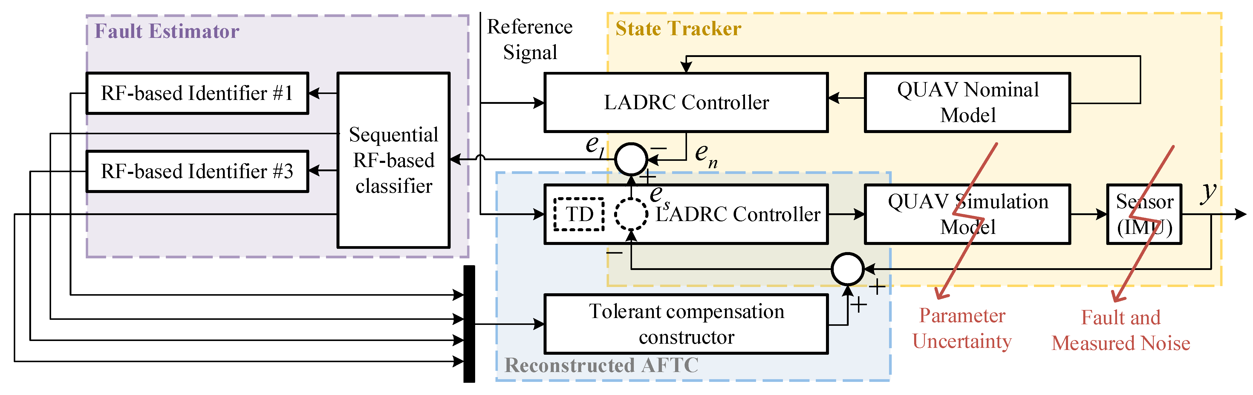
• A precise state tracker based on the linear extended state observer (LESO) and reference model is proposed, which can avoid the influence of maneuver changes, where the LESO ensures that the observed residual is within the noise level (under no-fault condition). The reference model makes the residual follow the transient changes, so as to eliminate the LESO delay effect caused by slow tracking.
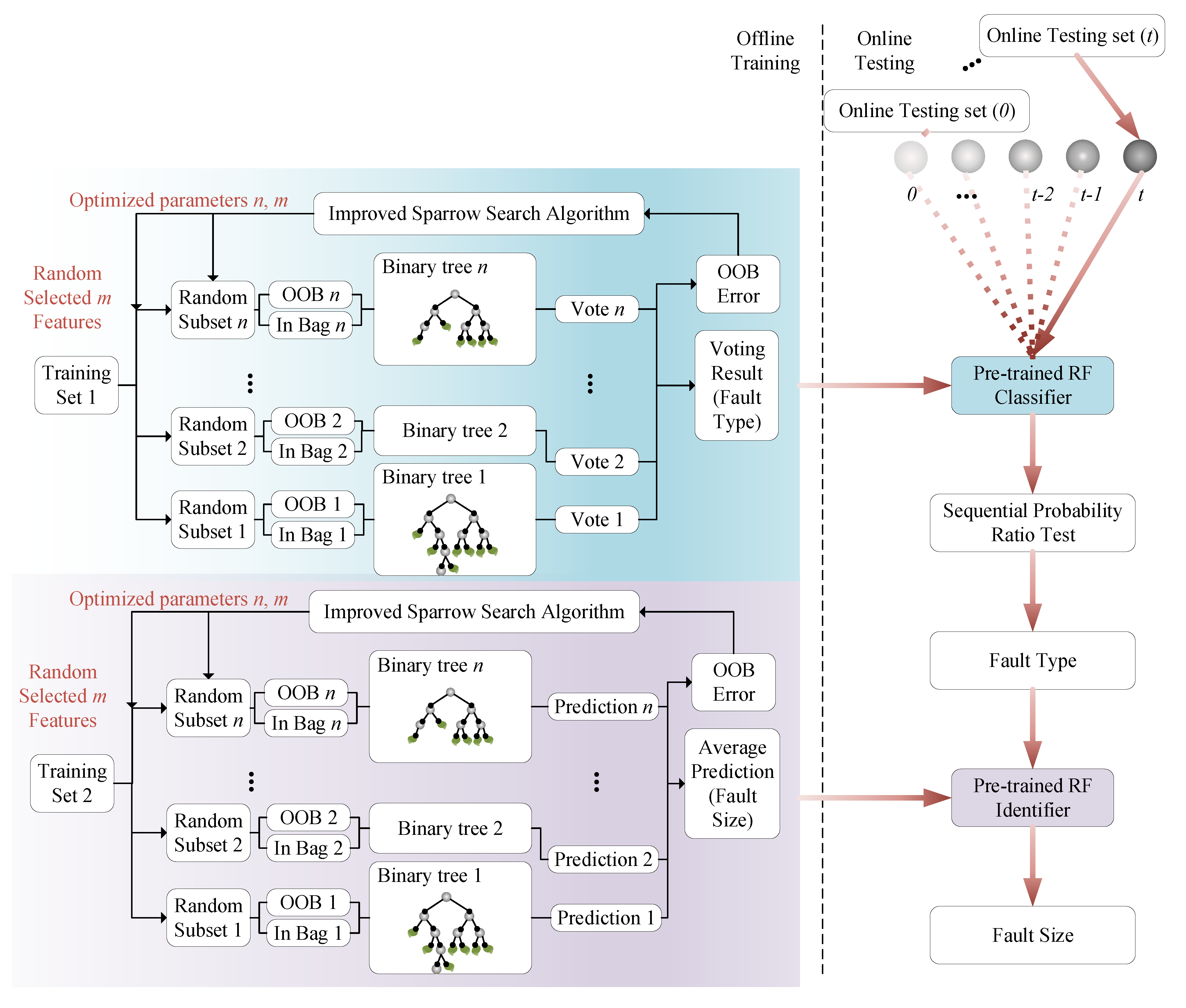
• Trained simply by a small amount of data, an precise fault estimator is designed. The auto sequential RF algorithm is proposed to realize real-time adaptive sensor fault diagnosis based on multi-sample, and the improved sparrow search algorithm (LSSA) is used for performing autonomous hyperparameter optimization.
• A high-performance AFTC approach combines the active compensation control strategy and the ADRC-based PFTC strategy is proposed for fault-tolerant control. Among them, the novel fault diagnosis algorithm provides the necessary fault information for the active compensation control strategy.

The paper is organized as follows. After a brief introduction, the modelling of the QUAV and the ADRC controller for the longitudinal channel, together with the sensor fault formulation, are addressed in Section 2. Section 3 details the complete ADRC-based AFTC control design in three stages. Then, in Section 4, the wide range of the simulation experiments of the developed fault tolerance controller is performed and analyzed. Finally, conclusions and future developments are reached in Section 5.

2. Mathematical Modeling of QUAV with Sensor Fault

In this section, QUAV mathematical modeling is provided to describe the drone’s motion. As the reference model, the nominal model established under ideal conditions lays the foundation for simulation experiments and state tracker design. The QUAV passive attitude controller is modeled based on parameter uncertainties and external disturbances. The sensor fault model discusses the change in QUAV output casued by typical type of fault, and supports the follow-up study on the AFTC method.

Remark 1.

Without losing generality, it is assumed that only the pitch angle sensor fails. Consequently, the longitudinal channel is considered in the QUAV attitude control modelling.

2.1. Modeling of the QUAV System

A QUAV is made up of four cross-placed rotors, as shown in Figure 1, with a symmetric pattern. Only the aerodynamic force on the rotor and its lift on the airframe are concerned during constructing the nominal model. After the QUAV is supposed to be a rigid body with uniform mass distribution, the modification of gravity acceleration is further ignored. QUAV is regarded as a mass point with three degrees of freedom (3-DOF) of motion on the x, y and z axes within the earth coordinate system $O_e{X}_e{Y}_e{Z}_e$. At the same time, it can be seen as a rigid body with 3-DOF roll, pitch and yaw movements in the body coordinate system $O_b{X}_b{Y}_b{Z}_b$.

As rendered in Figure 1, $\varphi$, $\theta$ and $\psi$ refer to the roll, pitch and yaw angle, respectively. Correspondingly, they are defined as the rotation angle of the body coordinate system around $x_b$, $y_b$ and $z_b$ axes. Rolling to the right, up along the nose and yawing to the right are denoted as the positive directions.

The Newton equation is used for analyzing the planar motion of the QUAV:

$$\begin{array}{c}\hfill \begin{array}{c}\ddot{x}=U_1(sin\theta cos\psi cos\varphi +sin\psi sin\varphi )/m-D_x{\dot{x}}^2/m\hfill \\ \ddot{y}=U_1(sin\theta cos\psi cos\varphi -cos\psi sin\varphi )/m-D_y{\dot{y}}^2/m\hfill \\ \ddot{z}=U_{1}cos\theta cos\varphi /m-g-D_z{\dot{z}}^2/m\hfill \end{array}\end{array}$$

(1)

where x, y and z represent the three-axis direction in the earth coordinate system, $U_1$ is the total lift force of rotors, $D_x$, $D_y$ and $D_z$ are the air-drag coefficients in the three-axis direction, m is the total mass, g indicates the gravitational acceleration.

The Euler equation is employed to analyze the rotation process:

$$\begin{array}{c}\hfill \begin{array}{c}\ddot{\varphi }=(J_y-J_z)\dot{\theta }\dot{\psi }/J_x+j_r\dot{\theta }(-{\omega }_1+{\omega }_2-{\omega }_3+{\omega }_4)/J_x+U_2/J_x\hfill \\ \ddot{\theta }=(J_z-J_x)\dot{\varphi }\dot{\psi }/J_y+j_r\dot{\varphi }(-{\omega }_1+{\omega }_2-{\omega }_3+{\omega }_4)/J_y+U_3/J_y\hfill \\ \ddot{\psi }=(J_x-J_y)\dot{\varphi }\dot{\theta }/J_z+U_4/J_z\hfill \end{array}\end{array}$$

(2)

where $J=diag(J_x,J_y,J_z)$ is the inertia tensor. $j_r$ is the propeller moment of inertia. $U_2$, $U_3$ and $U_4$ denote the roll, pitch and yaw moment of the body, respectively. $\omega$ is the rotor speed. A comprehensive nominal 6-DOF model of the QUAV is obtained by simultaneous (1) and (2).

The second-order system model is established as the actuator model to represent the rotor speed change, and the model transfer function $G_r\left(s\right)$ is written as:

$$G_r\left(s\right)=\frac{{\omega }_n^2}{s^2+2\xi {\omega }_{n}s+{\omega }_n^2}$$

(3)

where $\xi$ and ${\omega }_n$ are damping ratio and natural frequency, respectively.

2.2. Problem Formulation

To facilitate the control system design, the QUAV dynamic model is simplified as a longitudinal mode and thus reduced to a second-order system:

$$\ddot{\theta }=U_3/J_y$$

(4)

Denote $x_l={\left[x_1{x}_2\right]}^T={\left[\theta \dot{\theta }\right]}^T$ as the state variable, $y_l=\theta$ as the system output, $u_l={\left[F_1{F}_2{F}_3{F}_4\right]}^T$ as the control input. Equation (4) is further written in the state-space form:

$$\begin{array}{c}\hfill \begin{array}{c}{\dot{x}}_l=A_l{x}_l\left(t\right)+B_l{u}_l\left(t\right)\hfill \\ y_l\left(t\right)=C_l{x}_l\left(t\right)\hfill \end{array}\end{array}$$

(5)

With reference to the disturbance and sensor fault, (5) is further modified as:

$$\begin{array}{c}\hfill \begin{array}{c}{\dot{x}}_l=A_l{x}_l\left(t\right)+B_l{u}_l\left(t\right)+g(x_l,u_l,t)\hfill \\ y_l\left(t\right)=C_l{x}_l\left(t\right)+H\left(t\right)\hfill \end{array}\end{array}$$

(6)

where $g(x_l,u_l,t)$ represents both internal and external uncertainties in QUAV. Internal uncertainties include sensor noise and model parameter uncertainties, while external uncertainties include external disturbances such as gusts. $A_l=\left[\begin{array}{cc}0& 1\\ 0& 0\end{array}\right]$ is the nominal system state transition matrix. $B_l=\left[\begin{array}{cccc}0& 0& 0& 0\\ -\frac{l}{J_y}& -\frac{l}{J_y}& \frac{l}{J_y}& \frac{l}{J_y}\end{array}\right]$ and $C_l=\left[\begin{array}{cc}1& 0\end{array}\right]$ are the input and output matrices, respectively. l represents the distance from the rotor to the center of mass. $H\left(t\right)$ represents the sensor fault.

2.2.1. Quadrotor Attitude Passive Controller Modeling

In practice, time-consuming parameter tuning and fuzzy physical meaning limit the application of the ADRC [28]. Therefore, the idea of Linear ADRC (LADRC) was raised. By reducing the amount of parameters and endowing them with the significance of bandwidth, LADRC thus simplifies the tuning process [29]. Hence, this paper adopts the LADRC method for designing the passive controller, including tracking differentiator (TD), PD controller and LESO [30].

The controller structure is detailed in Figure 2, where the desired pitch angle is determined by the reference signal r.

Remark 2.

In the design of the PFTC, the sensor fault is ignored. In other words, term $H\left(t\right)$ in (6) is removed.

Inspired by the idea of the state observer in modern control theory, LESO expands the total disturbance $g(x_l,u_l,t)$ into a new state variable $z_3$ based on the state variables $z_1=\theta$ and $z_2=\dot{\theta }$ of the observation system. Using its special feedback mechanism, an extended state observer is established to observe the total disturbance.

After a new state variable $x_3=g(x_l,u_l,t)$ is introduced in (6), the second-order system is expanded into the following system:

$$\begin{array}{c}\hfill \begin{array}{c}{\dot{x}}_1=x_2\hfill \\ {\dot{x}}_2=x_3+b{u}_l\hfill \\ {\dot{x}}_3=g(x_l,u_l,t)\hfill \\ y_l=x_1\hfill \end{array}\end{array}$$

(7)

In order to better estimate the expanded system, the third-order LESO is conceived with the formula modified from (7):

$$\begin{array}{c}\hfill \begin{array}{c}e=z_1-y_l\hfill \\ \dot{z_1}=z_2-{\beta }_{1}e\hfill \\ \dot{z_2}=z_3-{\beta }_{2}e+b{u}_l\hfill \\ \dot{z_3}=-{\beta }_{3}e\hfill \end{array}\end{array}$$

(8)

where $z_1$ and $z_2$ are the pitch angle observation and its differential, respectively. $z_3$ refers to the total disturbance. e is the residual between the observation and the actual angle. b represents system parameters. ${\beta }_1$, ${\beta }_2$ and ${\beta }_3$ are tunable parameters.

To reduce the system overshoot caused by the step signal and to balance the response speed, TD is used to track and smooth the desired signal [31]. The filter factor h and speed factor $r^{\prime }$ are introduced into TD to soften the reference signal r, reduce the overshoot, and enhance controller stability. The expression is as follows:

$$\begin{array}{c}\hfill \begin{array}{c}e=z_1-y_l\hfill \\ {\theta }_1(t+1)={\theta }_1\left(t\right)+h{\theta }_2\left(t\right)\hfill \\ {\theta }_2(t+1)={\theta }_2\left(t\right)+\left[\left(-{r^{\prime }}^2{\theta }_1\left(t\right)-r\left(t\right)\right)-2r^{\prime }{\theta }_2\left(t\right)\right]\hfill \end{array}\end{array}$$

(9)

where ${\theta }_1\left(t\right)$ is the pitch angle output by TD at moment t, and ${\theta }_2\left(t\right)$ is its differential.

LADRC controller parameters are configured by the bandwidth parameterization: (1) Depending on the control bandwidth ${\omega }_c$, the system poles are positioned at $\left(-{\omega }_c,0\right)$; (2) The observer bandwidth is set to be ${\omega }_0=5\sim 10{\omega }_c$, and $\beta$ is set to meet ${\beta }_1=3{\omega }_0$, ${\beta }_2=3{{\omega }_0}^2$ and ${\beta }_3=3{{\omega }_0}^3$.

With proper $\beta$ setting, the residual $e\to 0$, and the ideal system can be written as:

$$\ddot{y_l}=x_3+b{u}_l$$

(10)

As illustrated in Figure 2, the controller is designed as $u_l=\frac{-z3}{b}+u_0$, which can be substituted into (10) and obtained $\ddot{y_l}=x_3-z_3+b{u}_0=e+b{u}_0\approx b{u}_0$. $u_0$ is the PD controller control output that is determined by:

$$u_0=K_p(r-z_1)+K_d(\dot{r}-z_2)$$

(11)

Assuming that the reference signal is a constant value, then $\dot{r}=0$, (11) can be rewritten as $\ddot{y}=bKp(r-\theta )-b{K}_d\dot{\theta }$. Finally, the transfer function can be written as:

$$G_{cl}\left(s\right)=\frac{Y\left(s\right)}{R\left(s\right)}=\frac{\Theta \left(s\right)}{R\left(s\right)}=\frac{b{K}_p}{s^2+b{K}_{d}s+b{K}_p}$$

(12)

where, when $K_p=\frac{{\omega }_c^2}{b},K_d=\frac{2\xi {\omega }_c^2}{b}$, the entire closed-loop system is equivalent to a standard second-order system. The above derivation demonstrates that the LADRC controller is stable.

2.2.2. Sensor Fault Description

For the feedback control, the QUAV attitude controller relies on the observation information obtained by the sensors to determine the system output. Therefore, the sensor fault directly causes the control loss or even controller failure. Although the sensor fault has been studied by researchers, it is usually considered as an interference term regardless of mechanism [32]. To solve the above problems, the possible types of the angle sensor fault are analyzed and summarized based on the QUAV characteristics. Afterwards, typical fault models are established for the pitch angle sensor.

Hard-Over Fault

Voltage or current bias in the sensor circuit is caused by a sudden temperature change. The fault presents as a large constant bias value $\Delta$ added to the non-faulty signal. The system response is suddenly unstable with an evident steady-state error.

Stuck Fault

An unstable transmission, even a permanent failure of sensors, is caused by a high overload. The measured signal maintains a certain value ${\theta }_s$ since the fault occurred.

Remark 3.

Generally, ${\theta }_s=\theta \left(t_f\right)$ is the last value measured by the sensor before it fails.

Slow-Varying Fault

The Parts are slowly worn out and age by the body vibration during long-term maneuvering, leading to the slow divergence of the sensor signal. The non-faulty signal is multiplied by a constant gain, which causes a slight fluctuation and a modest steady-state error at the beginning.

Outlier-Data Fault

Electromagnetic interference is produced by precise sensors with dense circuits and high-frequency switching power supply, causing local shock waves. Sensor signal deviates from the non-faulty signal in an instant. The system response is added with an impulse response, but recovers quickly without lasting impact.

The sensor fault is summarized and specified as follows:

$$\begin{array}{c}\hfill \begin{array}{c}{\theta }_{f,b}\left(t\right)=\theta \left(t\right)+{fal}_b\left(\Delta ,t_{f,b}\right)\hfill \\ {\theta }_{f,s}\left(t\right)=\theta \left(t\right)+{fal}_s\left(\theta \left(t\right),{\theta }_s,t_{f,s}\right)\hfill \\ {\theta }_{f,g}\left(t\right)=\theta \left(t\right)+{fal}_g\left(\theta \left(t\right),K_g,t_{f,g}\right)\hfill \\ {\theta }_{f,o}\left(t\right)=\theta \left(t\right)+{fal}_o\left({\delta }_o,t_{f,s}\right)\hfill \end{array}\end{array}$$

(13)

where the fault profile function $fal(•)$ is decided by $H\left(t\right)={\left[0fal(•)\right]}^T$ and satisfies:

$$fal\left(\theta \left(t\right),\Delta ,{\theta }_s,K_g,{\delta }_o,t_f\right)=\left[(K_g-1)·\theta \left(t\right)+\Delta +{\theta }_s+{\delta }_o\left(t_f\right)\right]·\beta (t-t_f)$$

(14)

where $\beta \left(t\right)=\left(sgn\left(t\right)+1\right)/2$ is the occurrence time profile function, $\Delta$ is a constant bias value, ${\theta }_s$ is a certain value, $K_g$ is a constant gain, ${\delta }_o\left(t\right)$ is an impulse signal.

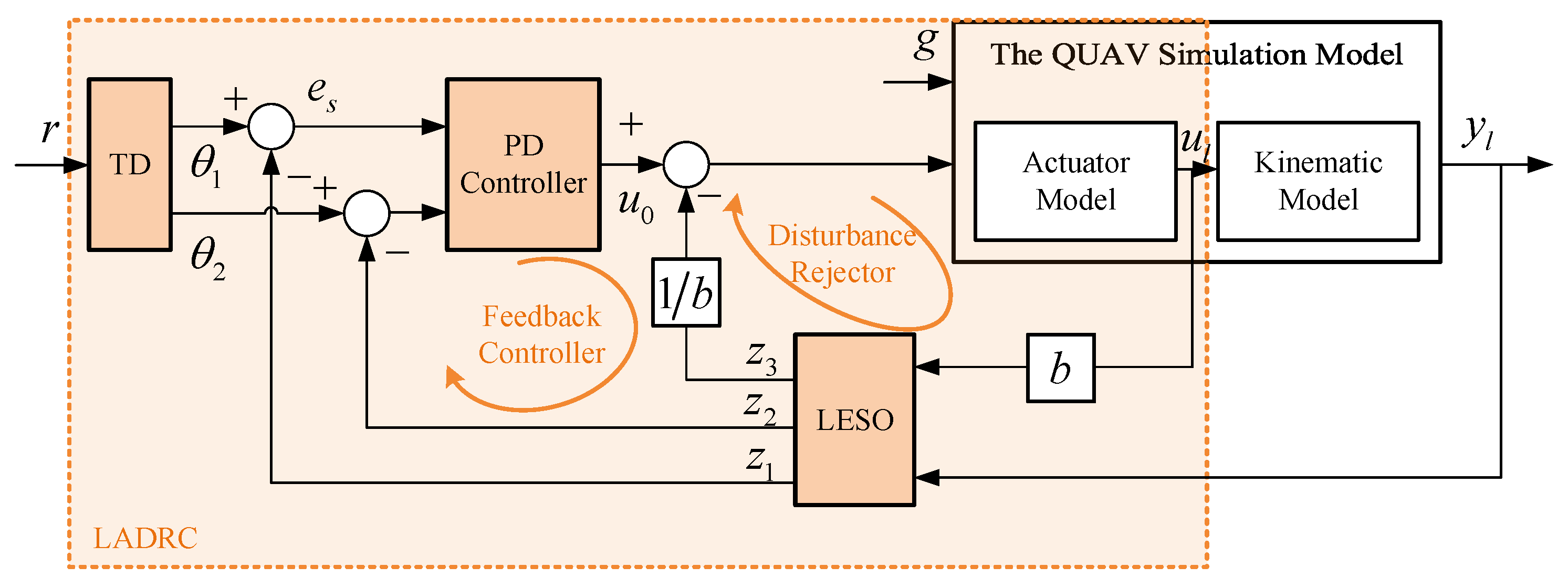
3. LADRC-Based Active-Tolerant Control Strategy

Although sensor measurement noise and small disturbances in the QUAV system are tolerated, the LADRC failed to handle most sensor fault according to the system response stated in Section 2.2.2. To address the above issue, a LADRC-based active fault-tolerant strategy is designed as shown in Figure 3. It is realized in three stages: (1) Semi-model-dependent state tracking. The residual is obtained from the difference between the nominal model output and the simulation model output, both of which are estimated by the LESO in advance. Not only is the reliable anti-interference ability retained to the internal and external disturbances of QUAV, but also the accurate state-tracking is reached by eliminating the maneuvering influence. (2) Intelligent fault estimating. If a fault beyond the tolerance of the passive controller occurs, the sequential RF-based classifier can separate the fault in real-time. The classification result is then used by the RF-based identifier to obtain the fault size. Among them, the LSSA is applied to automatically build the optimal fault diagnosis model, significantly reducing labor and time costs. (3) Fault-tolerant control compensating. The accurate fault information is used for the subsequent reconstruction of the fault-tolerant strategy to compensate for the LADRC control output. It should be noted that the core of this paper is to realize active control compensation through accurate and rapid real-time fault diagnosis, which is also the point of innovation.

3.1. Semi-Model-Dependent LESO State Tracker

Based on (1), (2) and (5), the nominal model is constructed. Once the LESO residual of the nominal model ($e_n$) and the simulation model ($e_s$) are obtained, the residual to be measured is calculated:

$$e_l=e_s-e_n$$

(15)

The resulting residual signal $e_l$ are processed as the input of FDS.

3.2. Model-Free Intelligent Fault Estimator

Prior to diagnosis, feature extraction is required to obtain sensitive features. Generally, feature extraction is realized by advanced signal processing technologies, including time and frequency domain methods, i.e., the principal component analysis and the Fourier transform. In the high dynamic and high maneuvering QUAV system, the sensor fault is usually presented by a vibration time sequence signal. For feature diversity and sensitivity are increased by extracting time-frequency features, the combination of wavelet packet translation (WPT) and statistical variable calculation is perfectly suitable for this task [33].

The residual signal to be measured is first decomposed by n-layer wavelet packet. After reconstruction at the m-th node, nine statistical parameters of each signal ${cfs}^m\left(e_l\right)$ are calculated respectively. The feature vector, with $(9\times 2^n)\times 1$ dimensions, of the residual signal is ultimately obtained:

$$X\left(t\right)={\left[F_1\left(t\right)F_2\left(t\right)\dots F_9\left(t\right)\right]}^T$$

(16)

where $F_i\left(t\right)={\left[f_i\left({cfs}^{m+1}\left({\theta }_f\left(t\right)\right)\right)f_i\left({cfs}^{m+2}\left({\theta }_f\left(t\right)\right)\right)\dots f_i\left({cfs}^{m+2^n}\left({\theta }_f\left(t\right)\right)\right)\right]}^T$, $m=2^n-2$, $n\ge 1$.

Remark 4.

Shape factor $f_1$, Margin factor $f_2$, Pulse factor $f_3$, Crest factor $f_4$, Absolute mean $f_5$, Mean square error $f_6$, Skewness $f_7$, Kurtosis $f_8$, and Mean square value $f_9$ are included in aforementioned parameters.

After extraction is realized by (16), features $X\left(t\right)$ are input into the intelligent fault estimator as training samples. As discussed in Section 1, the model-free FDE poses flaws in terms of poor generalization performance with small samples, bad real-time capacity, and high model construction cost. Once the sensor fault occurs during high dynamic and maneuvering flight, they can cause the QUAV attitude to diverge rapidly. In this paper, sequentiality is introduced into the RF to realize real-time fault diagnosis with small samples. And the heuristic algorithm is applied to perform auto model construction. Fault estimator implements fault isolation and identification by sequential RF classification and RF regression method, respectively. In addition, Levy mutation factor is introduced to achieve the auto-optimization of RF hyperparameter based on the LSSA, then the best fault estimator is obtained.

As illustrated in Figure 4, the fault diagnosis process involves two parts: offline training and online testing. The principal design ideas are outlined below.

3.2.1. Data Acquisition

The training set is composed of all signals with length $t_w$ under $k+1$ states in $[t_f-t_w,t_f+t_w]$ obtained by continuously intercepting the residual signal data, where the sampling time is $T_s$ and the intercept gap is $t_s$. The online test set is made up of residual signals from moment $t-t_w$ to present moment t. Both sets are formed as the final feature data set after extracting features, and the former is labeled.

3.2.2. Parameter Optimization Based on the Improved Sparrow Search Algorithm

In this paper, the RF model is composed of n binary trees. Each tree selects a certain number of features from the training set as the root node. After randomly extracting m candidate features, each tree splits and grows in the fastest declined direction of information entropy until the features are not separable. The separable point of the tree is called the node of the tree, with a quantity of d. In the case of a few features, the depth of the tree p is not explicitly limited. In this way, fault type and fault size are obtained by voting and mean value calculating, respectively.

Both precision and rapidity of the fault diagnosis are required by the AFTC. As in other artificial intelligence methods, RF has structure-affected accuracy and speed. When the RF is running, its time complexity and space complexity are $O(p·n)$ and $O(d·n)$, respectively. Once d is settled, p is determined by m. Thus, the RF operating speed is closely related to m and n. However, the mainstream manual tuning usually involves considerable professional knowledge and experience. In order to construct the optimal RF in a practical way, an automatic optimization algorithm for structural parameters is needed. Parameters include the number of decision trees contained in the RF and the number of feature variables used for binary tree ($d\le 2^{p-1}$) nodes. The SSA is a novel optimization algorithm based on the sparrow’s foraging and anti-predatory behavior [34]. Compared to other heuristic algorithms, i.e., the ant colony, bee colony and beetle antennae search algorithm [35], it has a better capacity for local development and global exploration. Furthermore, SSA performs better in optimizing multi-dimensional parameters.

To begin with, each structural parameter set is regarded as a sparrow. The optimum solution with minimum fitness is obtained iteratively by updating the population class and the individual position. In this paper, the mixed-performance fitness function is designed based on the requirements of the sensor fault diagnosis:

$$fi{t}_f\left(X\right)={\xi }_{1,f}oo{b}_f\left(X\right)+{\xi }_{2,f}{T}_f\left(X\right)$$

(17)

where X represents a parameter set, $T\left(X\right)$ is the processing time of the RF built with X, $oob\left(X\right)$ refers to the out of bag error, and $\xi$ are the mixed-performance attention coefficients.

The sparrow population is composed of producers and scroungers, while its class and regeneration are determined by the fitness order. Producers location is updated as follows:

$$X_{i,j}^{it+1}=\left\{\begin{array}{c}{X}_{i,j}^{it}·exp(-i/(\gamma ·i{t}_{max})),R_2<S_t\hfill \\ X_{i,j}^{it}+q·L,R_2>S_t\hfill \end{array}\right.$$

(18)

where the random numbers $R_2\in [0,1]$, $\gamma \in (0,1]$ and $Q\sim N(0,1)$. $S_t$ is the safety value. $it$ and $i{t}_{max}$ indicate the current iteration and the maximum iterations. All elements in L is 1.

Scrounger location updating is described as follows:

$$X_{i,j}^{it+1}=\left\{\begin{array}{c}Q·exp\left((X_{worst}^{it}-X_{i,j}^{it})/i^2\right),i>N_{pop}/2\hfill \\ X_{best}^{it+1}+|X_{i,j}^{it}-X_{best}^{it+1}|·A^{+}·L,i\le N_{pop}/2\hfill \end{array}\right.$$

(19)

where $X_{best}^{it+1}$ is the optimal producer location after update. $X_{worst}^{it}$ is the current global worst position. $N_{pop}$ is the population size. $A^{+}=A^T{\left(A{A}^T\right)}^{-1}$, where A is a real matrix with elements in $\{\pm 1\}$.

In particular, each sparrow has same awareness of danger. Sparrows who aware of danger update their position as:

$$X_{i,j}^{it+1}=\left\{\begin{array}{c}{X}_{best}^{it}+\lambda ·|X_{i,j}^{i}t-X_{best}^{it}|,fi{t}_{f,i}>fi{t}_{f,g}\hfill \\ X_{i,j}^{it}+K·\left[|X_{i,j}^{it}-X_{worst}^{it}|/(fi{t}_{f,i}-fi{t}_{f,w}+ϵ)\right],fi{t}_{f,i}=fi{t}_{f,g}\hfill \end{array}\right.$$

(20)

where $X_{best}^{it}$ indicates the global best position. The random numbers $\lambda \sim N(0,1)$ and $K\sim [-1,1]$. $fi{t}_{f,g}$ and $fi{t}_{f,w}$ represent the minimum and maximum fitness, respectively. $ϵ$ is an extremely small constant.

According to (19), the Vanilla SSA lacks an effective mutation mechanism. A producer can be directly replaced by any superior scrounger, making individuals easily attracted by the local optimum. For improvement, the Levy flight is introduced to modify the individual position, enhancing their local escape ability and accelerating the convergence [36]. The tournament selection is first used to select individuals, and the Levy mutation is then performed:

$$X_i^{it+1}=X_i^{it}+(X_i^{it}-X_{best}^{it})\otimes Levy\left(2\right)$$

(21)

where $Levy\left(2\right)$ is the Levy mutation factor. If fitness declines after the update, the update is accepted, otherwise the original position is retained.

3.2.3. Fault Isolation and Identification Based on the Auto Sequential RF

Once the optimal RF model is trained, online test data are input into each tree for classification or regression. The sliding window method is used by most of the existing real-time algorithms to realize the multi-sample diagnosis, while its own time delay is ignored. In this paper, to reduce the time delay and accomplish an adaptive multi-sample diagnosis, the RF classifier is enhanced by introducing the sequentiality. More specifically, the online-test data is input into the trained classification RF, and the probability output of each fault corresponding to the current state is obtained according to the voting results:

$$h_{n,m}\left(x_t^k\right)=\frac{1}{n}\left(\sum _{i=1}^n{x}_t^0\left(S_m^i\right)\sum _{i=1}^n{x}_t^1\left(S_m^i\right)\cdots \sum _{i=1}^n{x}_t^k\left(S_m^i\right)\right)$$

(22)

where k is the fault label. $x_t^k$ is 1 when the binary tree votes for fault k at moment t, otherwise it is 0. $S_m^i$ is the i-th binary tree classification strategy based on m randomly selected feature variables.

The fault type is assumed as discrete random variable $X=0,1,2,\cdots ,k$, and the probability distribution of $h_{n,m}\left(X_t\right)$ in (22) is satisfied at moment t. For the k-th type fault, the sequential probability ratio statistic at moment t is computed [37]:

$${LR}_t={LR}_{t-t_s}+ln\left(P_k\left(X_t\right)/P_0\left(X_t\right)\right)$$

(23)

where $P_k\left(X\right)$ is the probability of k-th type fault, and $P_0\left(X\right)$ represents the probability of normal state.

${LR}_t$ is calculated iteratively in accordance with (23) for sequential possibility ratio test (SPRT):

• If $L{R}_t\le ln\left(P_{FNR}/(1-P_{FPR})\right)$, the test is terminated and the system is ruled normal, where $P_{FNR}$ and $P_{FPR}$ are the false negative rate and false positive rate, respectively.
• If $L{R}_t\ge ln\left((1-P_{FNR})/P_{FPR}\right)$, the test is terminated and the k-th fault is justified to occur the system.
• If $ln\left((1-P_{FNR})/P_{FPR}\right)\le {LR}_t\le ln\left(P_{FNR}/(1-P_{FPR})\right)$, then the system is determined of the same state as the previous, and next sampling sample is waited to test.

Most notably, the detecting and lasting delay can be caused by the negative value accumulation below the negative threshold and the positive value accumulation above the positive threshold, respectively. In order to eliminate the delay, the iteration of $L{R}_t$ is modified:

$$L{R}_t=\left\{\begin{array}{c}0,L{R}_t<0,X_t=0\hfill \\ L{R}_t,L{R}_t\ge 0,X_t=0\hfill \\ L{R}_{t-1},\dot{L{R}_t}\ge 0,X_t\ne 0\hfill \\ L{R}_t,\dot{L{R}_t}<0,X_t\ne 0\hfill \end{array}\right.$$

(24)

where $\dot{L{R}_t}$ indicates the increment in $L{R}_t$.

Because the aforementioned test can only examine the single fault occurrence, test rule is improved in this paper application of the multiple fault detection. To summarize, the detailed flow of the auto sequential RF online fault isolation and identification is listed in Algorithm 25.

Algorithm 1 The auto sequential RF-based online fault isolation procedure

Obtain the online test set $X_{tst}$ after the feature extraction; Given the sampling time $T_s$, intercept gap $t_s$, false negative rate $P_{FNR}$, false positive rate $P_{FPR}$; Input: The online test set $X_{tst}$ Output: Fault type $Y_{fin}\left(end\right)$ Initialization: The sequential probability ratio statistic $LR=0$, final type $Y_{fin}=0$, justified result $Y_{tst}=0$. 1:  for each sampling time i in $\left[1,((t-t_w)/T_s)+1\right]$ do 2:     Obtain votes $\sum x_i^k\left(S_m\right)$ through the pre-trained classification RF. 3:     Calculate fault probability distribution $h\left(x_i^k\right)$ according to (22); 4: end for 5: Calculate $LR(1,k)=ln\left(P_k\left(X_1\right)/P_0\left(X_i\right)\right)$; 6: while$i\le ((t-t_w)/T_s)+1$do 7:     if $Y_{fin}(i-1)$ is 0 then 8:           for each fault type j in $[1,k]$ do 9:              compute $LR(i,j)$ according to (23) and (24); 10:            Obtain the justified result $Y_{tst}(i,j)$ according to SPRT; 11:         end for 12:         if $Y_{tst}$ is 0 then 13:            $Y_{fin}\left(i\right)=0$; 14:            $j_{cha}=\left\{j\mid Y_{tst}(i,j)\ne 0\right\}$; 15:         else if $\exists !j_{cha}:Y_{tst}(i,j_{cha})\ne 0$ then 16:            $Y_{fin}\left(i\right)=j_{cha}$; 17:         else 18:            $Y_{fin}\left(i\right)=\left\{j_{cha}\mid max\left(LR(i,j_{cha})\right)\right\}$; 19:         end if 20:     else 21:         Compute $LR(i,Y_{fin}(i-1))$ according to (23) and (24); 22:         Obtain the justified result $Y_{tst}(i,Y_{fin}(i-1))$ according to SPRT; 23:         $Y_{fin}\left(i\right)=Y_{tst}(i,Y_{fin}(i-1))$; 24:     end if 25: end while

3.3. Reconfigurable Tolerant Compensation Constructor

After the sensor fault is identified successfully, the reconstructed AFTC strategy is obtained according to the fault-tolerant compensating. The control structure is described in Figure 3.

The AFTC strategy is designed as:

$${\theta }_{AFTC}\left(t\right)=\left\{\begin{array}{c}\theta \left(t\right),0\le t\le t_f\hfill \\ {\theta }_f\left(t\right),t_f\le t\le t_d\hfill \\ {\theta }_{comp}\left(t\right),t\ge t_d\hfill \end{array}\right.$$

(25)

where $t_d$ is when the fault estimator determines the fault, ${\theta }_{comp}\left(t\right)$ is the control compensation, which is determined by the fault-tolerant compensation strategy for a specific fault:

$$\begin{array}{c}\hfill \begin{array}{c}{\theta }_{comp,b}\left(t\right)=\theta \left(t\right)+\Delta -{\Delta }_{est}\left(t_d\right)\hfill \\ {\theta }_{comp,s}\left(t\right)={\theta }_{est}\left(t\right)\hfill \\ {\theta }_{comp,g}\left(t\right)=K_g\theta \left(t\right)/K_{est}\left(t_d\right)\hfill \\ {\theta }_{comp,o}\left(t\right)=\theta \left(t\right)\hfill \end{array}\end{array}$$

(26)

where ${\Delta }_{est}$ is the size of the identified hard-over fault, $K_{est}$ is the gain of the identified slow-varying fault, and ${\theta }_{est}$ is the observed value of the system regardless of the state feedback.

Remark 5.

As a short-term fault, outlier-data fault is considered to require no additional compensation, for the reliable sensor data is easy to get by either filtering or information fusion.

4. Simulation Results

To verify the effectiveness of the proposed AFTC method, the simulation trials of the QUAV attitude control against the sensor fault are presented in this section. High-fidelity simulations is conducted to simulate an actual QUAV. As the T-MOTOR’s AntiGravity MN2214 engine is adopted, this QUAV is fitted with 1045 carbon fiber composite propellers and a 16.8 V, 4S lithium polymer battery. The nominal parameters are defined as given in

Table 1. QUAV nominal model parameters.

Parameter	Symbol	Value
Mass (kg)	m	1.44
Inertia tensor (kg m2)	$diag(J_x,J_y,J_z)$	$\left[\begin{array}{ccc}0.0097& 0& 0\\ 0& 0.0097& 0\\ 0& 0& 0.0178\end{array}\right]$
Propeller moment of inertia (kg m2)	$j_r$	$1.04\times {10}^{-4}$

, and the simulation model contains 10% parameter uncertainty. The damping ratio of the actuator model is set as 0.9 and the natural frequency is set to 98 rad. The inertial measurement unit (IMU) is used as the sensor, and the measurement noise of 0.0045rad is accounted for the model. The initial status of the QUAV is assumed $x=z=0$, $h=0\mathrm{m}$, $V=0\mathrm{m}/\mathrm{s}$, $\theta =\varphi =\psi =0^{\circ }$, $u=0$. In the nominal system design, the controller and the LESO observer are stabilized by setting the cut-off frequencies ${\omega }_c=20\mathrm{rad}$ and ${\omega }_0=100\mathrm{rad}$ respectively. The desired pitch angle signal is chosen as the reference signal, with a 10${}^{\circ }$ amplitude and 3 s simulation time. At the same time, given the change in flight conditions caused by the maneuver change request, the expected pitch angle changes to 8${}^{\circ }$ at 2 s.

When the above parameters are disturbed and external disturbances occur, as depicted in Figure 5a, the simulation response shows that the settling time is 0.49 s (with an error in 2%). In order to explore the LESO disturbance estimation ability, a 0.01 N·m moment disturbance is injected into the system to simulate external gust disturbance. The injection time is 1.5 s, when the QUAV maintains a steady flight. According to the disturbance estimation curve depicted in Figure 5b, the LESO designed in this paper estimates the external disturbance well.

The sensor fault may occur at any time in the normal flight process, and it arises more easily as time increases. In preset working conditions, the range of hard-over and slow-varying fault sizes are $[{1.275}^{\circ },5^{\circ }]$ and $(0.90,0.97)\bigcup (1.04,1.10)$, respectively. And the stuck- and outlier-data faults are 10${}^{\circ }$ and 40${}^{\circ }$, respectively. To guarantee the universality of the training data for the FDS, the data are obtained by injection of faults at 1.5s. For the sampling time of 0.001 s (The frequency of IMU is 1 kHz), the interception interval is 0.02 s and the data range is 0.2 s. After the raw training data are processed by three-layer WPT using the db2 wavelet, nine statistical parameters of eight nodes in the third layer are then computed. A total of 72 features are extracted. As the normal state, Hard-over fault, stuck fault, slow-varying fault and outlier-data fault are labeled as 0, 1, 2, 3 and 4, respectively, an the training set is eventually obtained.

4.1. State Tracking Tests

The direct residual is derived by subtracting the pitch angle signal generated by the nominal model from that measured in the simulation model. Which is greatly affected by the modeling accuracy. Since the LESO is model-independent, the residual signal may converge to the measured noise level in the normal state, but cannot completely track the maneuver changes. To demonstrate the superiority of the LESO and reference model combination, the direct and LESO residuals are used for the fault data respectively to explore the fault representation capacity.

The training sets for fault isolation are obtained by feature extraction of direct and LESO residuals with sensor fault. Where the fault sizes are 2${}^{\circ }$, 10${}^{\circ }$, 0.94 and 40${}^{\circ }$ respectively. The importance of each feature $X_i$ is expressed by a Gini index score $VI{M}_i^{Gini}$, which indicates the average change in node splitting impurity in all binary trees. Then the feature importance of the two training sets is plotted in Figure 6. Furthermore, the size of the most sensitive (most important) feature of each training data is given in Figure 7.

Results show that the LESO residual has a smaller intra-class variance and a larger inter-class distance, with a less overlap of feature dispersion. Based on the LESO residual features, different types of faults are better distinguished, resulting in a better fault representation capacity. This is because LESO can eliminate certain high-frequency interference as a low-pass filter, generating a residual signal noise smaller than the direct residual. Due to the integration, the residual signal fluctuation has inertia and is no longer highly oscillatory. In addition, the sudden sensor fault usually appears as a high-frequency signal [33]. Figure 6a shows that the application of high-frequency features increases, and further proves that the LESO residual signal can describe fault signal more comprehensively.

4.2. Performance Metrics

In order to make the performance of the fault diagnosis algorithm more intuitive, four main metrics are employed in this paper. Among them, False positive rate (FPR), Precision rate, Recall rate and False negative rate (FNR) are widely used in multi-class classification:

$$\begin{array}{c}\hfill \begin{array}{c}FPR=\frac{FP}{TN+FP}\hfill \\ Precision=\frac{TP}{TP+FP}\hfill \\ Recall=\frac{TP}{TP+FN}\hfill \\ FNR=\frac{FN}{TP+FN}\hfill \end{array}\end{array}$$

(27)

where the samples can be divided into four categories according to the combination of their real type and the predicted type of the classifier: TP is true positive, FN is false negative, FP is false positive and TN is true negative.

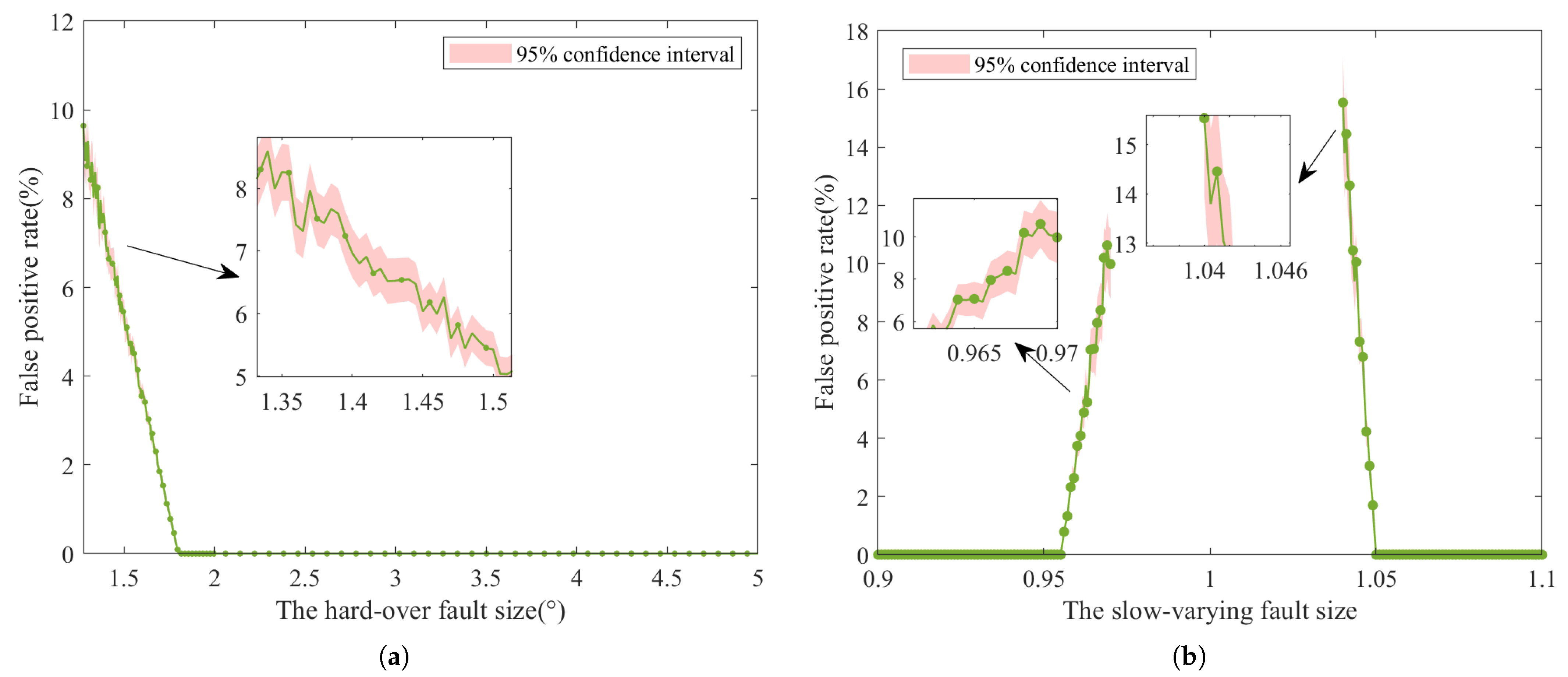
4.3. Fault Estimation Tests

In the offline training, the fault estimator first isolates faults based on the RF classifier to determine the fault type. If the hard-over fault or slow-varying fault is justified, the fault size is further obtained by the fault identification based on the RF identifier. Therefore, a pre-trained RF classifier and two pre-trained RF identifiers are needed, which are constructed separately. For model optimization purposes, the LSSA is used to optimize the RF structure parameters. The amount of training data, classification complexity and regression precision are involved in the parameter search space. Mixed performance attention coefficients are generally defined as a constant that makes terms have a same order of magnitude. Particularly, the training set composition and optimization related settings of above three learning machines are listed in

Table 2. Offline training settings and results of RF model.

Model	Fault Size	Data per Class 1	Parameter Search Space		Attention Coefficient		Optimal Parameters		Error
			n	m	${\mathit{\xi }}_1$	${\mathit{\xi }}_2$	n	m
The RF classifier	${\Delta }_b=2^{\circ }$,${\theta }_s={10}^{\circ }$, $K_l=0.94$,${\delta }_o={40}^{\circ }$	500	$(0,500]$	$[2:2:8]$	1	0	500	8	0 (OOB error)
The RF identifier for hard-over fault	${\Delta }_b\in \{{1.275}^{\circ },{1.5}^{\circ },2^{\circ },{2.5}^{\circ },$ $3^{\circ },{3.5}^{\circ },4^{\circ },{4.5}^{\circ },5^{\circ }\}$	9	$(0,300]$	$[2:2:28]$	1	${10}^{-3}$	136	12	0.0068 (MSE error)
The RF identifier for slow-varying fault	$K_l\in \{1.1,1.0,0.95,0.9\}$	9	$(0,300]$	$[2:2:28]$	1	${10}^{-3}$	92	12	0.0004 (MSE error)

¹ Number of training data with the same label.

. It needs to be claimed that the auto sequential RF algorithm relies on large-scale voting bases to ensure the accuracy of statistical probability. Therefore, the construction of RF classifier ignores the influence of processing time, but pursues the accuracy as much as possible.

The optimal structure parameters and accuracy of above three models are obtained after training according to Table 2. In the process of training, parameters of the LSSA are set as follows: the population size $N_{pop}=5$, the maximum iterations $i{t}_{max}=50$, the safety value $S_t=0.8$, the proportion of producers $P_d=0.2$ and the proportion of those aware of danger $S_d=0.2$. The results show that the optimal RF model can accurately distinguish different faults in the offline situation. For simplicity, the following analysis is based on the hard-over fault. Compared to the performance of Vinalla SSA in Figure 8b, the LSSA method can jump out of the local optimum and get the global optimum earlier. As the prediction follows the actual value perfectly in Figure 8c, the optimal RF identifier can accurately and quickly identify the fault size. In addition, the optimal RF identifier requires only a few training data matching a small part of the amplitude to predict perfectly, which demonstrates its high capacity for prediction using small samples.

To explore the optimal RF classifier’s generalization performance to the same type of fault, the above classification model is used to classify the fault sets with changing sizes. The results presented in

Table 3. Classification results of RF classifier for faults with different sizes.

Fault Type	Fault Size	Accuracy (%)	Hybrid Accuracy (%) ${}^1$
Hard-over fault	1.275${}^{\circ }$	100	100
	2${}^{\circ }$	100
	3${}^{\circ }$	100
	4${}^{\circ }$	100
	5${}^{\circ }$	100
Slow-varying fault	1.10	86.20	88.0516
	1.06	100
	1.04	89.20
	0.97	89.60
	0.94	100
	0.90	53.40

¹ The accuracy of slow varying fault with bound size refers to the accuracy of corresponding hard-over fault or normal state.

show that the optimal RF classifier can accurately distinguish the hard-over fault of different sizes. Moreover, it can isolate a slow-varying fault with others in most cases. However, at the bounds of fault size, the classifier effect has a certain degree of deterioration. This is because, if the slow-varying fault is too small, it will be covered by noise and confused with the normal state. If it is too large, it will evolve into a hard-over fault, which is difficult for the classifier to distinguish. However, the performance loss of fault isolation caused by these two situations will not affect the fault-tolerant compensation. The former can be eliminated by the passive ADRC based controller, while the latter is directly compensated by the identified hard-over fault. Meanwhile, to better present the classifier’s performance, the following hybrid generalization accuracy index (hereinafter referred to as hybrid accuracy) is proposed to globally assess the classifier’s precision and generalization capability:

$$\begin{array}{c}\hfill \begin{array}{c}Ac{c}_m=\sum Ac{c}_s·{\widehat{\omega }}_s\hfill \\ {\omega }_s=1/\left(\sqrt{2\pi }\sigma \right)·exp\left(-{(s-\mu )}^2/2{\mu }^2\right)\hfill \\ {\widehat{\omega }}_s={\omega }_s/\sum \omega \hfill \end{array}\end{array}$$

(28)

where $Ac{c}_s$ is the accuracy when the fault size is s, $\widehat{{\omega }_s}$ is the importance function, $s\sim N(\mu ,{\sigma }^2)$, $\mu$ is set to the training set fault size, and the standard deviation is defined as $\sigma =min(s_{max}-\mu ,\mu -s_{min})/3$. $s_{max}$ and $s_{min}$ are the bounds of the fault size.

Based on the design of the RF-based offline fault diagnosis system, further real-time diagnosis is needed. After $P_{FNR}=P_{FPR}=0.01$ are set, the auto sequential RF-based classifier proposed in this paper is used for online fault diagnosis. To prove that the proposed method can reduce the time delay while ensuring the accuracy, the RF classifier combined with the sliding window method is used for comparative experiments. The performance metrics of the proposed and contrast method are listed in

Table 4. Real-time fault diagnosis result.

Performance Metric	Auto Sequential RF					Contrast
	Normal	Hard-Over	Stuck	Slow-Varying	Outlier-Data	Normal	Hard-Over	Stuck	Slow-Varying	Outlier-Data
FPR(%)	4.52	0	0	1.87	0	0.40	0	6.75	4.43	0.36
Precision(%)	84.70	100	100	91.63	100	98.43	100	78.73	83.37	98.44
Recall(%)	100	92.52	100	81.93	100	100	72.36	100	88.87	91
FNR(%)	0	7.48	0	18.07	0	0	27.64	0	11.13	9

. It can be seen that the auto sequential RF provides better performance in most cases. However, the recall rate of slow varying fault is slightly lower and its missed diagnosis rate is higher. Meanwhile, the normal state false alarm rate is higher and its precision rate is lower. In order to further investigate the reasons for the above results, Detailed results of different fault sizes and types are provided in

Table 5. Real-time fault diagnosis result of the hard-over fault.

Method	Fault Size (%)	Accuracy (%)	Time Delay (s)	Fault Probability (%)					Hybrid Accuracy (%)
				Hard-Over	Stuck	Slow-Varying	Outlier-Data	Normal
Auto Sequential RF	1.275	62.6	0.04	62.6	0	37.4	0	0	99.6
	2	100	0.02	100	0	0	0	0
	3	100	0.02	100	0	0	0	0
	4	100	0.02	100	0	0	0	0
	5	100	0.02	100	0	0	0	0
Contrast	1.275	0	0.1	0	11.4	88.6	0	0	91.8
	2	92.8	0.1	92.8	0	0	7.2	0
	3	86.4	0.1	86.4	13.6	0	0	0
	4	92.6	0.1	92.6	7.4	0	0	0
	5	90	0.1	90	10	0	0	0

,

Table 6. Real-time fault diagnosis result of the slow-varying fault.

Method	Fault Size	Accuracy (%)	Time Delay (s)	Fault Probability (%)					Hybrid Accuracy (%)
				Hard-Over	Stuck	Slow-Varying	Outlier-Data	Normal
Auto Sequential RF	1.10	100	0.02	0	0	100	0	0	86.05
	1.06	100	0.02	0	0	100	0	0
	1.04	53.6	0.02	0	0	53.6	0	46.4
	0.97	38.0	0.02	0	0	38.0	0	62.0
	0.94	100	0.02	0	0	100	0	0
	0.90	100	0.02	0	0	100	0	0
Contrast	1.10	90.6	0.1	0	9.4	90.6	0	0	81.95
	1.06	91.4	0.1	0	8.6	91.4	0	0
	1.04	86.2	0.1	0	7.6	86.2	0	6.2
	0.97	84.6	0.1	0	12.0	84.6	0	3.4
	0.94	89.4	0.1	0	10.6	89.4	0	0
	0.90	91.0	0.1	0	9.0	91.0	0	0

and

Table 7. Real-time fault diagnosis result of the stuck fault and the outlier-data fault.

Fault Type	Method 1	Accuracy (%)	Fault Probability (%)					Early Diagnosis (%)	Time Delay (s)
			Hard-Over	Stuck	Slow-Varying	Outlier-Data	Normal
Stuck	A	100	0	100	0	0	0	0	0.04
	B	94.6	0	100	0	0	0	5.4	0.1
Outlier-data	A	100	0	0	0	100	0	0	0.02
	B	91.0	0	9.0	0	91.0	0	9.0	0.1

¹ A and B refers to the auto sequential RF-based method and the contrast method, respectively.

. It can be seen that the proposed method can diagnose the fault more precisely within a very short time, and has lower missed diagnosis and misdiagnosis rates. Although the accuracy of the auto sequential RF classifier is lower in the slow-varying fault diagnosis, it is still superior. On the one hand, the contrast method allows early diagnosis. Once the stuck fault is judged, the fault-tolerant system will inject corresponding compensation immediately. The wrong compensation leads to faster divergence of the whole system and even serious consequences. On the other hand, although the proposed method may misdiagnose the developed slow-varying fault, the fault-tolerant demands can be met by judging it as the hard-over fault, and vice versa.

For the purpose of a proof of the effectiveness of the proposed fault diagnosis algorithm, Monte Carlo experiments [38] are carried out with varying fault sizes and random noises. A total of 295 groups of hard-over faults are set, and their constant bias value of hard-over fault changes from 1.275${}^{\circ }$ to 2${}^{\circ }$ with a 0.005${}^{\circ }$ interval and from 2${}^{\circ }$ to 5${}^{\circ }$ with a 0.02${}^{\circ }$ interval. A total of 295 groups of slow-varying faults are set, and their constant gain value varies from 0.9 to 0.97 and from 1.04 to 1.1 with a 0.0005 interval. The proposed fault diagnosis algorithm runs five times under random noise for each fault size. The diagnosis results show that only the false alarm of slow-varying fault will appear in the diagnosis of the hard-over fault, while only the false alarm of normal state will appear in the diagnosis of the slow-varying fault, which is consistent with the previous analysis results. According to FPR results indicated in Figure 9, the false alarm rate keeps low when the fault is obvious. Therefore, the proposed algorithm is indicated for good generalization ability and strong robustness.

Considering that QUAVs are resource constrained devices, the memory occupation of the proposed fault algorithm is discussed. For each type of fault, the memory occupied by the offline-formed auto sequential RF classifier is only 2 KB. The memory of the random forest identifier for hard-over fault and slow-varying fault is 11 KB. The size of sensor signal feature data processed by the diagnosis algorithm at one time is 33 KB. The Pixhawk flight control board commonly used by QUAV is equipped with a 4 GB memory card, which is more than sufficient for the implementation of the fault diagnosis algorithm.

4.4. Fault-Tolerant Control Tests

The high-performance fault-tolerant control is realized as follows: As soon as a sensor fault occurs, the residual will rapidly follow the state changes, the fault information will be precisely estimated, and the compensation strategy will reconstruct to control the QUAV attitude perfectly. Hence, the AFTC controller needs to tackle faults with all possible sizes. Additionally, the fault can occur at any time, even when the reference signal changes. To illustrate the proposed method can solve above concerns, fault with different size and type is injected into the QUAV system at different times for the simulation. The above simulation results are organized by fault type in Figure 10, Figure 11 and Figure 12 and the following analyses are conducted.

Unlike the oscillation, large static error, and even divergence in the PFTC pitch response curve, the proposed AFTC curves indicate improved control performance under all simulation conditions. For the hard-over fault, the settling time increases when the fault size decreases, while the overshoot is on the opposite. The main reasons are as follows: (1) relatively small faults are more difficult to distinguish and take a longer time, leading to compensation delays; (2) larger faults are detected faster, but the system needs more time to recover gradually. It can be seen from Figure 10a that when the fault occurs with an unchanged reference signal, the settling time is only 0.176 s. For the slow-varying fault, when the fault size is at the upper and lower bounds ($K_l=0.90,1.10$), it is treated as a hard-over fault. The settling time in Figure 11a is 0.155 s, supporting the statement mentioned in Section 4.3 that a proper misdiagnosis of the fault estimator can be tolerated. In addition, the disturbance of the reference signal change makes no affection on the AFTC controller when the fault and maneuver change occur at the same time.

As a complex and high-dimensional nonlinear system, QUAV has sensor fault that is easy to cause, interact and develop between themselves. This requires the proposed AFTC to have a certain fault-tolerance capability for sequential multiple faults. Consequently, seven representative scenarios in

Table 8. Representative scenarios of the sequential multiple faults.

	Fault Type	Occurrence Time (s)	Fault Size
Scenario 1 (S1)	Slow-varying	1.5	0.94
	Hard-over	2	2${}^{\circ }$
Scenario 2 (S2)	Slow-varying	1.5	1.06
	Hard-over	2	4${}^{\circ }$
Scenario 3 (S3)	Hard-over	1.5	2${}^{\circ }$
	Hard-over	2	4${}^{\circ }$
Scenario 4 (S4)	Slow-varying	1.5	0.94
	Slow-varying	2	0.90
Scenario 5 (S5)	Hard-over	1.5	4${}^{\circ }$
	Stuck	2	$\theta \left(2\right)$
Scenario 6 (S6)	Slow-varying	1.5	0.94
	Stuck	2	$\theta \left(2\right)$
Scenario 7 (S7)	Outlier-data	1.5	40${}^{\circ }$
	Stuck	2	$\theta \left(2\right)$

are developed for simulation verification.

The results in Figure 13 reveal that AFTC is capable of handling sequential multiple faults. Although the cumulative compensation mechanism has certain limits, the extremely rapid settling speed of the proposed method makes it possible to compensate for multiple faults within short periods of time.

5. Conclusions

To summarize, this paper investigates the attitude control of the QUAV with sensor fault. By combining the ADRC design method with the auto sequential RF diagnosis method, an AFTC method is proposed. Its anti-disturbance ability and control performance are explored.

• A semi-model-dependent state tracker is obtained by innovatively combining the LESO with reference model. The slow-tracking problem is solved, that residual signal changes are easily confounded when faults occur and reference signal changes.
• Based on the accurate classification and prediction of the RF, an adaptive real-time fault diagnosis for the multi-sample data is achieved. To autonomously construct the fault estimator, the LSSA optimization achieves high speed and accuracy.
• The control effect is verified by experiments using the high fidelity simulation model. The results show that the proposed ADRC-based AFTC method can track the desired attitude signal precisely and quickly, and that performance requirements are met.

Although the proposed method can effectively deal with the typical sensor fault, there is still room for development and progress. Since the probability of fault in auto sequential RF is calculated cumulatively, composite fault (when signals occur simultaneously or show time overlaps) cannot be distinguished. The slow-varying fault is weak, but it still has a sudden hop at the beginning and an unchanged slope. It cannot fully represent the gradually changing fault. The above problems require further consideration and resolution.

6. Patents

The fault diagnosis method proposed in this paper has been licensed as a patent in China (Patent No.: ZL202111058850.3).

References

1. Walter, C.A.; Braun, A.; Fotopoulos, G. Impact of three-dimensional attitude variations of an unmanned aerial vehicle magnetometry system on magnetic data quality. Geophys. Prospect. 2019, 67, 465–479. [Google Scholar] [CrossRef]
2. Wang, Z.X.; Zhao, J.; Cai, Z.H.; Wang, Y.X.; Liu, N.J. Onboard actuator model-based Incremental Nonlinear Dyn.amic Inversion for quadrotor attitude control: Method and application. Chin. J. Aeronaut. 2021, 34, 216–227. [Google Scholar] [CrossRef]
3. Yu, Z.Q.; Zhang, Y.M.; Jiang, B.; Fu, J.; Jin, Y. A review on fault-tolerant cooperative control of multiple unmanned aerial vehicles. Chin. J. Aeronaut. 2021, 35, 1–18. [Google Scholar] [CrossRef]
4. Xu, Y.; Yang, H.; Jiang, B. Fault-tolerant control for a class of linear interconnected hyperbolic systems by boundary feedback. J. Frankl. Inst. 2019, 356, 5630–5651. [Google Scholar] [CrossRef]
5. Nguyen, N.P.; Xuan Mung, N.; Ha, L.N.N.T.; Hong, S.K. Fault-Tolerant Control for Hexacopter UAV Using Adaptive Algorithm with Severe Faults. Aerospace 2022, 9, 304. [Google Scholar] [CrossRef]
6. Zou, Y.; Xia, K. Robust Fault-Tolerant Control for Underactuated Takeoff and Landing UAVs. IEEE Trans. Aerosp. Electron. Syst. 2020, 56, 3545–3555. [Google Scholar] [CrossRef]
7. Rudin, K.; Ducard, G.J.; Siegwart, R.Y. Active fault-tolerant control with imperfect fault detection information: Applications to UAVs. IEEE Trans. Aerosp. Electron. Syst. 2019, 56, 2792–2805. [Google Scholar] [CrossRef]
8. Abbaspour, A.; Yen, K.K.; Forouzannezhad, P.; Sargolzaei, A. A Neural Adaptive Approach for Active Fault-Tolerant Control Design in UAV. IEEE Trans. Syst. Man Cybern. Syst. 2020, 50, 3401–3411. [Google Scholar] [CrossRef]
9. Zeghlache, S.; Mekki, H.; Bouguerra, A.; Djerioui, A. Actuator fault tolerant control using adaptive RBFNN fuzzy sliding mode controller for coaxial octorotor UAV. ISA Trans. 2018, 80, 267–278. [Google Scholar] [CrossRef]
10. Nguyen, N.P.; Hong, S.K. Fault diagnosis and fault-tolerant control scheme for quadcopter UAVs with a total loss of actuator. Energies 2019, 12, 1139. [Google Scholar] [CrossRef] [Green Version]
11. Zhang, W.Q.; Dong, C.Y.; Ran, M.P.; Liu, Y. Fully distributed time-varying formation tracking control for multiple quadrotor vehicles via finite-time convergent extended state observer. Chin. J. Aeronaut. 2020, 33, 2907–2920. [Google Scholar] [CrossRef]
12. Zhang, J.Y.; Rizzoni, G.; Cordoba-Arenas, A.; Amodio, A.; Aksun-Guvenc, B. Model-based diagnosis and fault tolerant control for ensuring torque functional safety of pedal-by-wire systems. Control Eng. Pract. 2017, 61, 255–269. [Google Scholar] [CrossRef]
13. Kang, J.; Xiong, Z.; Wang, R.; Zhang, L. Multi-Layer Fault-Tolerant Robust Filter for Integrated Navigation in Launch Inertial Coordinate System. Aerospace 2022, 9, 282. [Google Scholar] [CrossRef]
14. Yu, P.; Cao, J.; Jegatheesan, V.; Shu, L. Activated sludge process faults diagnosis based on an improved particle filter algorithm. Process Saf. Environ. Protect. 2019, 127, 66–72. [Google Scholar] [CrossRef]
15. Yan, K.; Chen, M.; Jiang, B.; Wu, Q.X. Robust adaptive active fault-tolerant control of UAH with unknown disturbances and actuator faults. Int. J. Adapt. Control Signal Process. 2019, 33, 684–711. [Google Scholar] [CrossRef]
16. Zhu, Q.Y.; Li, Z.Y.; Tan, X.T.; Xie, D.B.; Dai, W. Sensors fault diagnosis and active fault-tolerant control for PMSM drive systems based on a composite sliding mode observer. Energies 2019, 12, 1695. [Google Scholar] [CrossRef]
17. Shao, X.L.; Liu, J.; Cao, H.L.; Shen, C.; Wang, H.L. Robust dynamic surface trajectory tracking control for a quadrotor UAV via extended state observer. Int. J. Robust Nonlinear Control 2018, 28, 2700–2719. [Google Scholar] [CrossRef]
18. Meng, Q.; Hou, Z.S. Active Disturbance Rejection Based Repetitive Learning Control With Applications in Power Inverters. IEEE Trans. Control Syst. Technol. 2020, 29, 2038–2048. [Google Scholar] [CrossRef]
19. Zhao, Z.H.; Cao, D.; Yang, J.; Wang, H.M. High-order sliding mode observer-based trajectory tracking control for a quadrotor UAV with uncertain dynamics. Nonlinear Dyn. 2020, 102, 2583–2596. [Google Scholar] [CrossRef]
20. Xu, Q.Z.; Wang, Z.S.; Zhen, Z.Y. Information fusion estimation-based path following control of quadrotor UAVs subjected to Gaussian random disturbance. ISA Trans. 2020, 99, 84–94. [Google Scholar] [CrossRef]
21. Zhou, L.S.; Ma, L.L.; Wang, J.Z. Fault tolerant control for a class of nonlinear system based on active disturbance rejection control and rbf neural networks. In Proceedings of the 36th Chinese Control Conference, Dalian, China, 26–28 July 2017; pp. 7321–7326. [Google Scholar]
22. Amin, A.A.; Mahmood-ul Hasan, K. Robust active fault-tolerant control for internal combustion gas engine for air–fuel ratio control with statistical regression-based observer model. Meas. Control 2019, 52, 1179–1194. [Google Scholar] [CrossRef]
23. Ijaz, S.; Yan, L.; Hamayun, M.T.; Shi, C. Active fault tolerant control scheme for aircraft with dissimilar redundant actuation system subject to hydraulic failure. J. Frankl. Inst. 2019, 356, 1302–1332. [Google Scholar] [CrossRef]
24. Al Younes, Y.; Noura, H.; Rabhi, A.; El Hajjaji, A. Actuator fault-diagnosis and fault-tolerant-control using intelligent-output-estimator applied on quadrotor uav. In Proceedings of the 2019 International Conference on Unmanned Aircraft Systems, Atlanta, GA, USA, 11–14 June 2019; pp. 413–420. [Google Scholar]
25. Zhong, Y.J.; Liu, Z.X.; Zhang, Y.M.; Zhang, W.; Zuo, J.Y. Active fault-tolerant tracking control of a quadrotor with model uncertainties and actuator faults. Front. Inform. Technol. Elect. Eng. 2019, 20, 95–106. [Google Scholar] [CrossRef]
26. Wang, B.; Shen, Y.Y.; Zhang, Y.M. Active fault-tolerant control for a quadrotor helicopter against actuator faults and model uncertainties. Aerosp. Sci. Technol. 2020, 99, 105745. [Google Scholar] [CrossRef]
27. Zhou, M.; Wang, K.; Wang, Y.; Luo, K.J.L.; Fu, H.Y.; Si, L. Online condition diagnosis for a two-stage gearbox machinery of an aerospace utilization system using an ensemble multi-fault features indexing approach. Chin. J. Aeronaut. 2019, 32, 1100–1110. [Google Scholar] [CrossRef]
28. Gao, K.; Song, J.; Wang, X.; Li, H. Fractional-order proportional-integral-derivative linear active disturbance rejection control design and parameter optimization for hypersonic vehicles with actuator faults. Tsinghua Sci. Technol. 2020, 26, 9–23. [Google Scholar] [CrossRef]
29. Liu, C.Q.; Luo, G.Z.; Chen, Z.; Tu, W.C.; Qiu, C. A linear ADRC-based robust high-dynamic double-loop servo system for aircraft electro-mechanical actuators. Chin. J. Aeronaut. 2019, 32, 2174–2187. [Google Scholar] [CrossRef]
30. Gao, K.; Song, J.; Yang, E. Stability analysis of the high-order nonlinear extended state observers for a class of nonlinear control systems. Trans. Inst. Meas. Control 2019, 41, 4370–4379. [Google Scholar] [CrossRef]
31. Zhao, K.; Song, J.; Hu, Y.; Xu, X.; Liu, Y. Deep Deterministic Policy Gradient-Based Active Disturbance Rejection Controller for Quad-Rotor UAVs. Mathematics 2022, 10, 2686. [Google Scholar] [CrossRef]
32. Tan, J.; Fan, Y.; Yan, P.; Wang, C.; Feng, H. Sliding mode fault tolerant control for unmanned aerial vehicle with sensor and actuator faults. Sensors 2019, 19, 643. [Google Scholar] [CrossRef] [Green Version]
33. Ai, S.J.; Song, J.; Cai, G.B. Diagnosis of Sensor Faults in Hypersonic Vehicles Using Wavelet Packet Translation Based Support Vector Regressive Classifier. IEEE Trans. Reliab. 2021, 70, 901–915. [Google Scholar] [CrossRef]
34. Xue, J.K.; Shen, B. A novel swarm intelligence optimization approach: sparrow search algorithm. Syst. Sci. Control Eng. 2020, 8, 22–34. [Google Scholar] [CrossRef]
35. Li, X.Q.; Jiang, H.K.; Niu, M.G.; Wang, R.X. An enhanced selective ensemble deep learning method for rolling bearing fault diagnosis with beetle antennae search algorithm. Mech. Syst. Signal Process. 2020, 142, 106752. [Google Scholar] [CrossRef]
36. Pathak, Y.; Arya, K.; Tiwari, S. Feature selection for image steganalysis using levy flight-based grey wolf optimization. Multimed. Tools Appl. 2019, 78, 1473–1494. [Google Scholar] [CrossRef]
37. Guo, P.; Infield, D. Wind Turbine Power Curve Modeling and Monitoring With Gaussian Process and SPRT. IEEE Trans. Sustain. Energy 2020, 11, 107–115. [Google Scholar] [CrossRef]
38. Asadi, D. Model-based Fault Detection and Identification of a Quadrotor with Rotor Fault. Int. J. Aeronaut. Space Sci. 2022, 1–13. [Google Scholar] [CrossRef]
Figure 1. Intuitive representation of the Euler angle for QUAV.
Aerospace 09 00518 g001
Figure 2. Layout of the Quadrotor LADRC controller.
Aerospace 09 00518 g002
Figure 3. Overview of the LADRC-based AFTC for the QUAV with sensor fault.
Aerospace 09 00518 g003
Figure 4. The flow of the sequential RF-based fault isolation and identification system.
Aerospace 09 00518 g004
Figure 5. System simulation in normal state with internal and external disturbances. (a) Pitch angle response of the simulation model in normal state. (b) LESO external disturbance estimation results.
Aerospace 09 00518 g005
Figure 6. The feature importance distribution. (a) The LESO residual features. (b) The direct residual features. The x-axis is the feature number. For a feature with the i-th statistical parameter of the m-th WPT node, it is numbered as 72. If the nodes are sorted according to the frequency band, the order is: 7, 8, 10, 9, 13, 14, 12, 11 (nodes from the third layer after three-layer WPT).
Aerospace 09 00518 g006
Figure 7. The distribution of the most sensitive feature in different training set. (a) Feature distribution of nominal model with LESO. (b) Feature distribution of nominal model.
Aerospace 09 00518 g007
Figure 8. The offline training results of hard-over fault. (a) Parameter and objective space of the RF structure parameter optimization. (b) Fitness curves of the LSSA and the Vanilla SSA. (c) Prediction of the trained RF identifier. The test data used for (c) are obtained by injecting the hard-over fault with different size into the QUAV system 160 times, where fault size is between 1 to 5 with an interval of 0.25.
Aerospace 09 00518 g008
Figure 9. Fault diagnosis result of Monte Carlo experiments. (a) The FPR of the slow-varying fault when the hard-over fault occurs. (b) The FPR of the normal state when the slow-varying fault occurs.
Aerospace 09 00518 g009
Figure 10. Comparative results of the proposed ADRC-based active fault-tolerant control for QUAV with the hard-over fault occurred at (a) 1.5 s. (b) 2 s.
Aerospace 09 00518 g010
Figure 11. Comparative results of the proposed ADRC-based active fault-tolerant control for QUAV with the slow-varying fault occurred at (a) 1.5 s. (b) 2 s.
Aerospace 09 00518 g011
Figure 12. Comparative results of the proposed ADRC-based active fault-tolerant control for QUAV. (a) With the stuck fault. (b) With the outlier-data fault.
Aerospace 09 00518 g012
Figure 13. Comparative results of the proposed ADRC-based active fault-tolerant control for QUAV in various scenarios.
Aerospace 09 00518 g013