
Aerodynamic Interference on Trim Characteristics of Quad-Tiltrotor Aircraft


Abstract
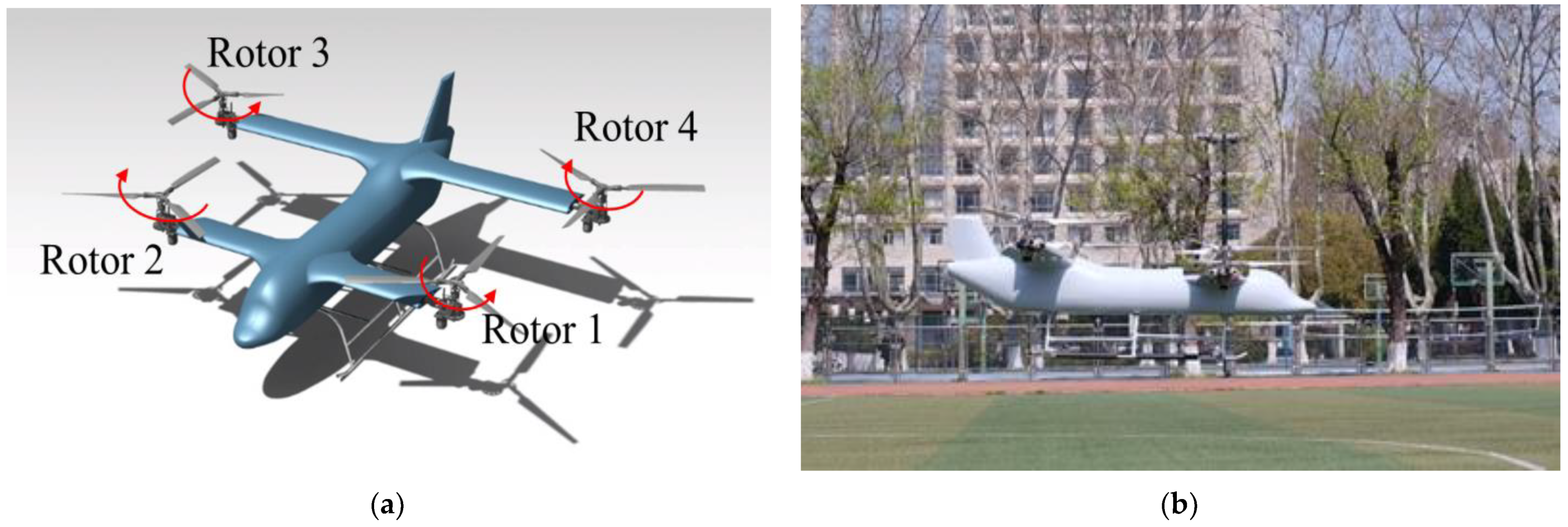
:1. Introduction
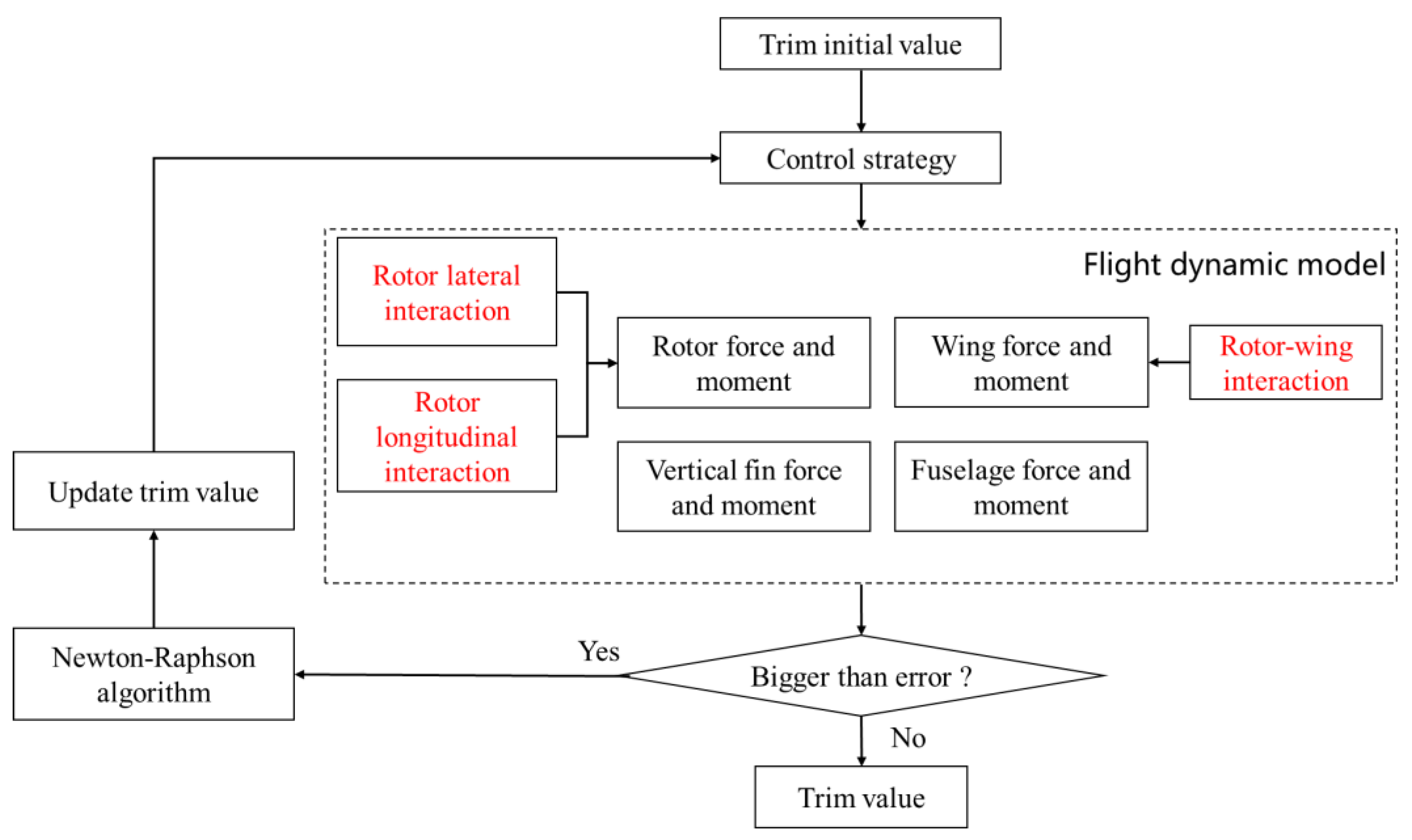
2. Flight Dynamics Model and Validation
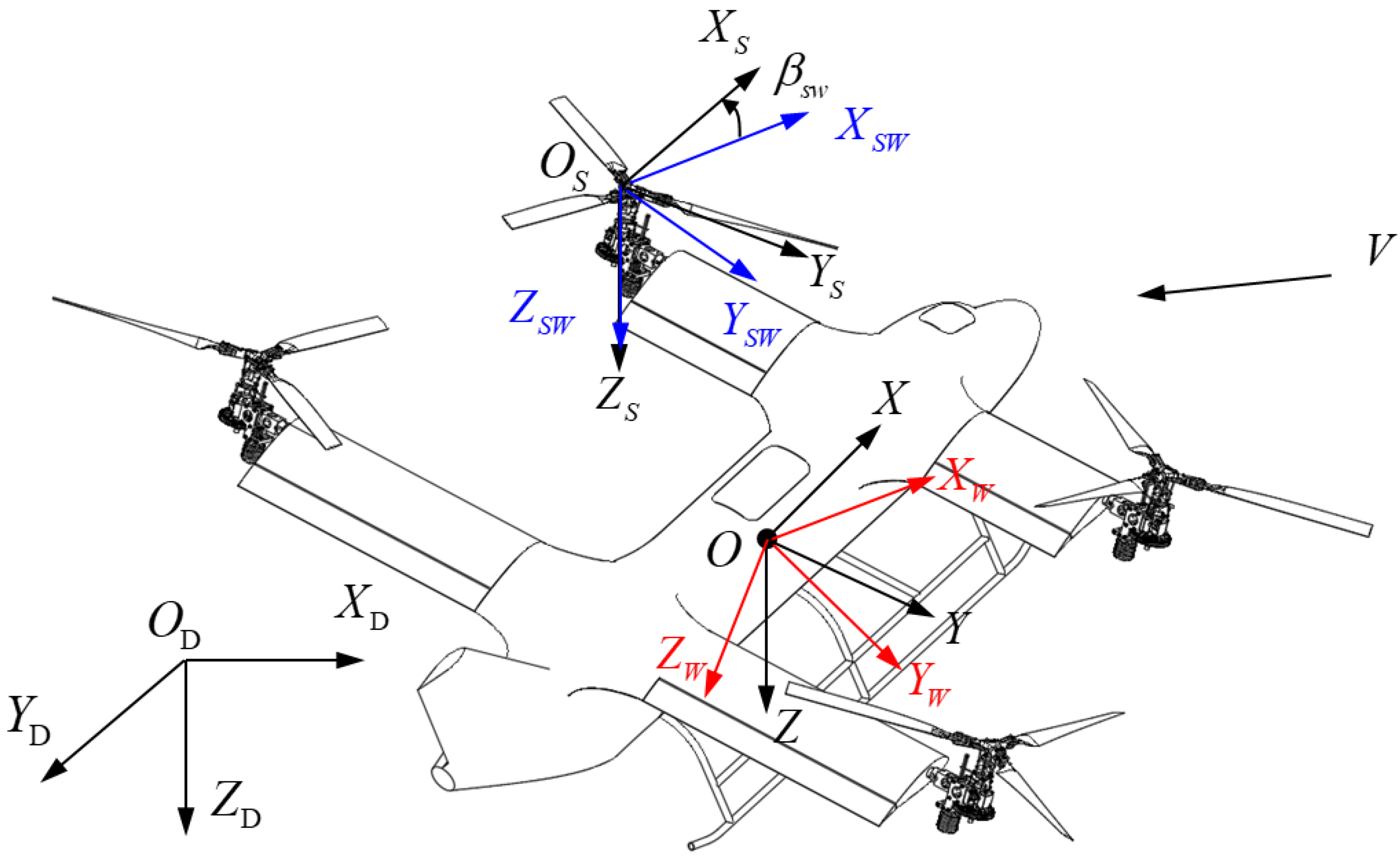
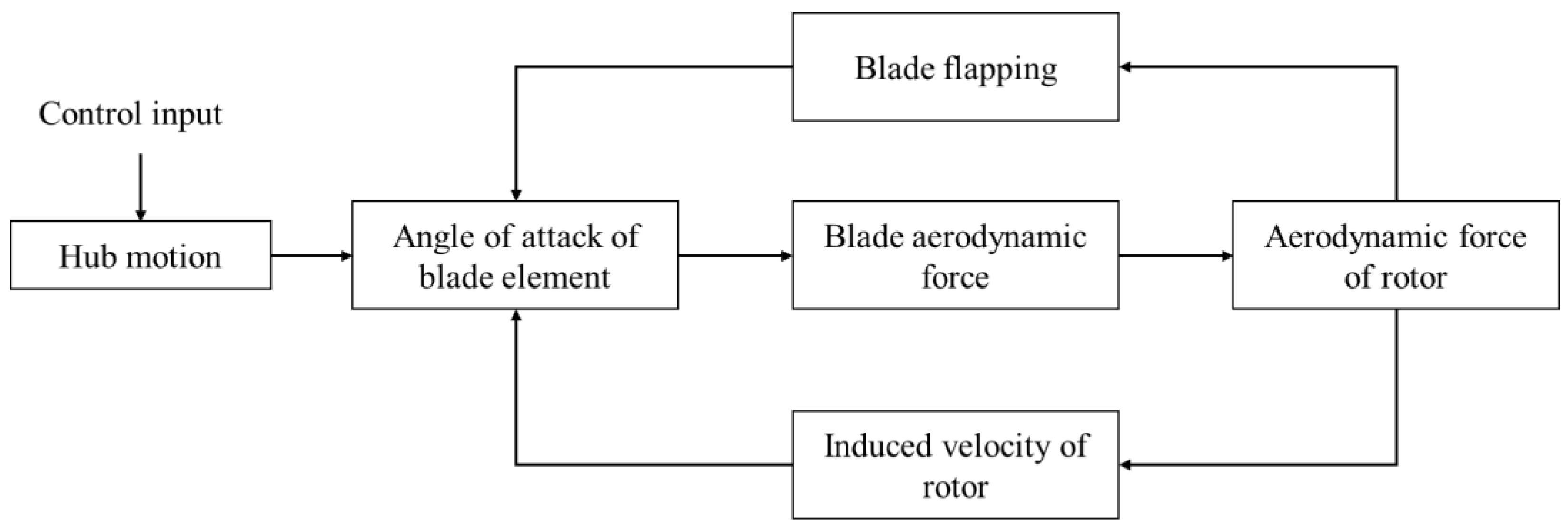
2.1. Rotor Model
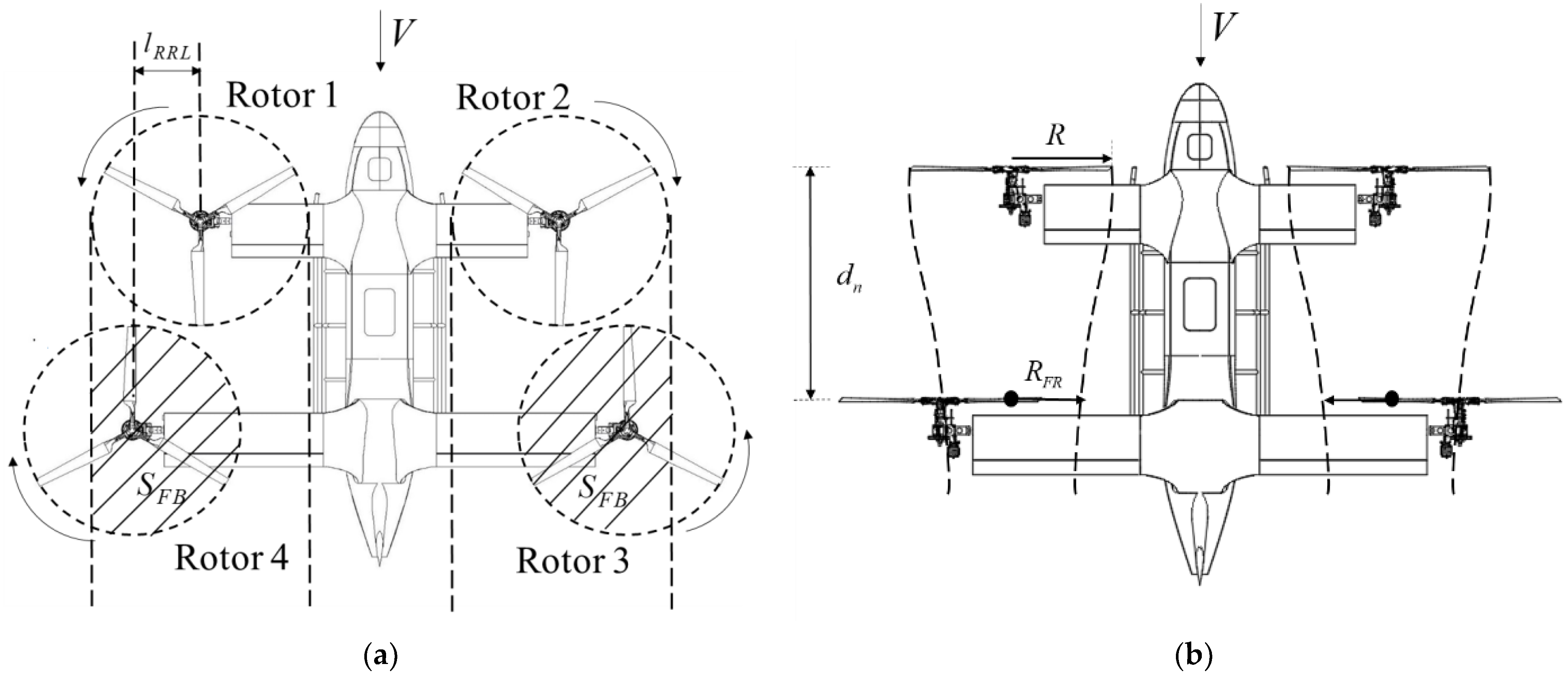
2.1.1. Lateral Interaction
2.1.2. Longitudinal Interaction
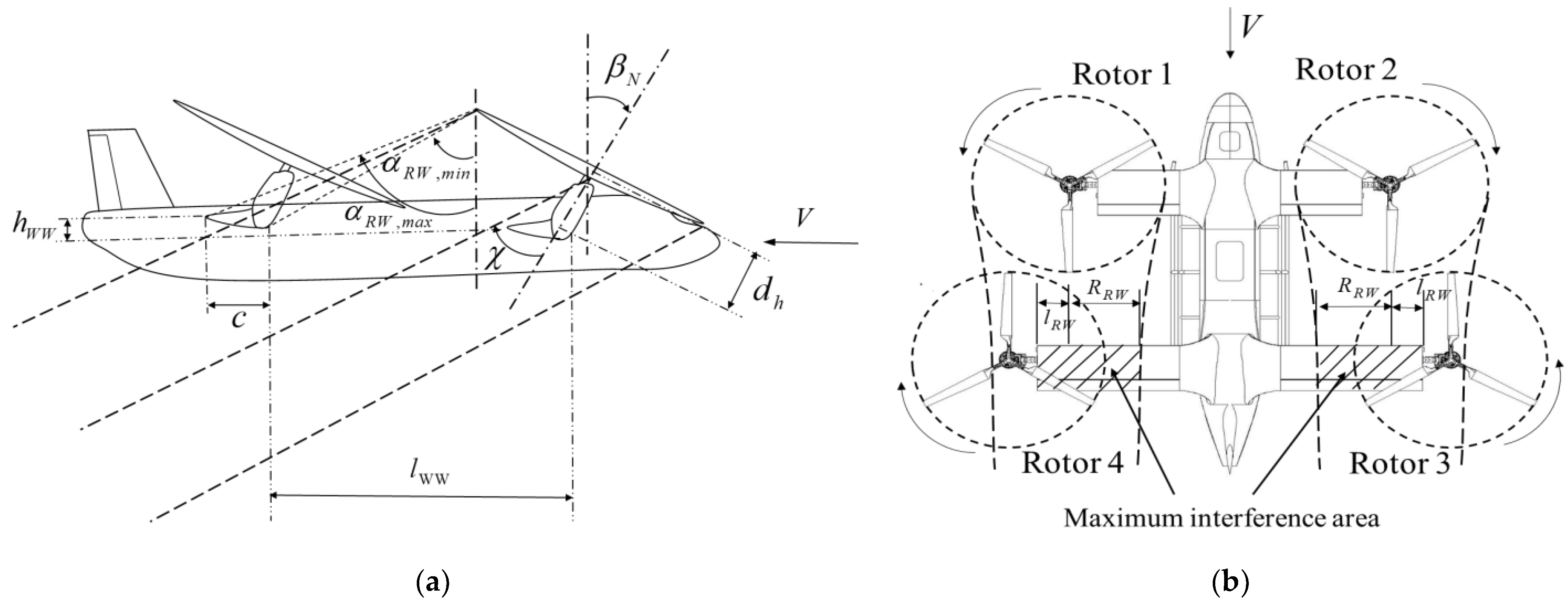
2.2. Wing Model
2.2.1. Rotor–Wing Interaction: Type 1
2.2.2. Rotor–Wing Interaction: Type 2
2.3. Model of Other Components
2.4. Integrated Equations of the Vehicle
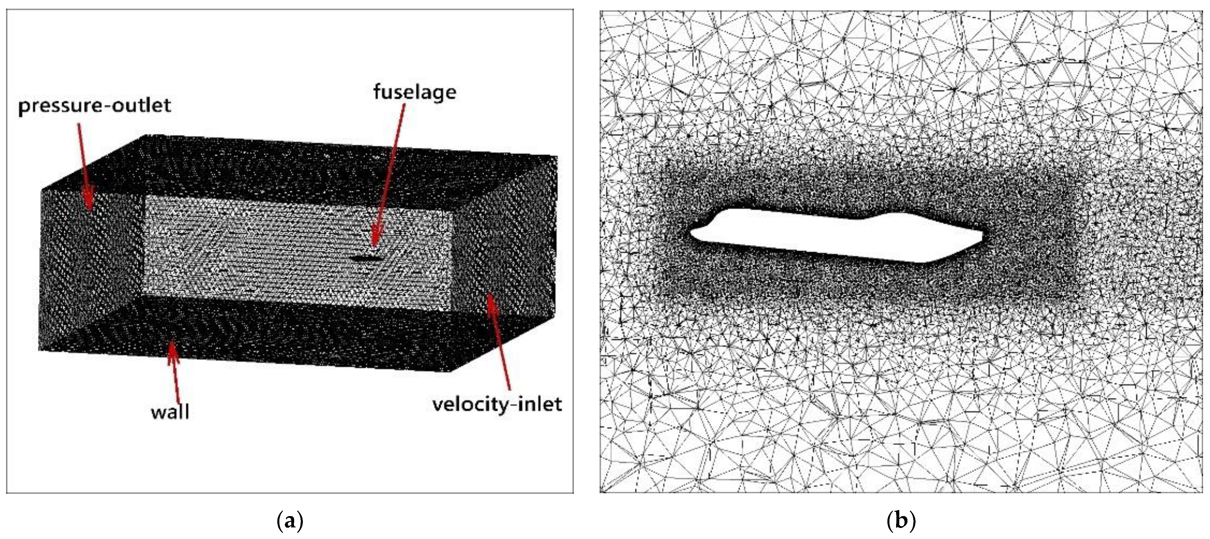
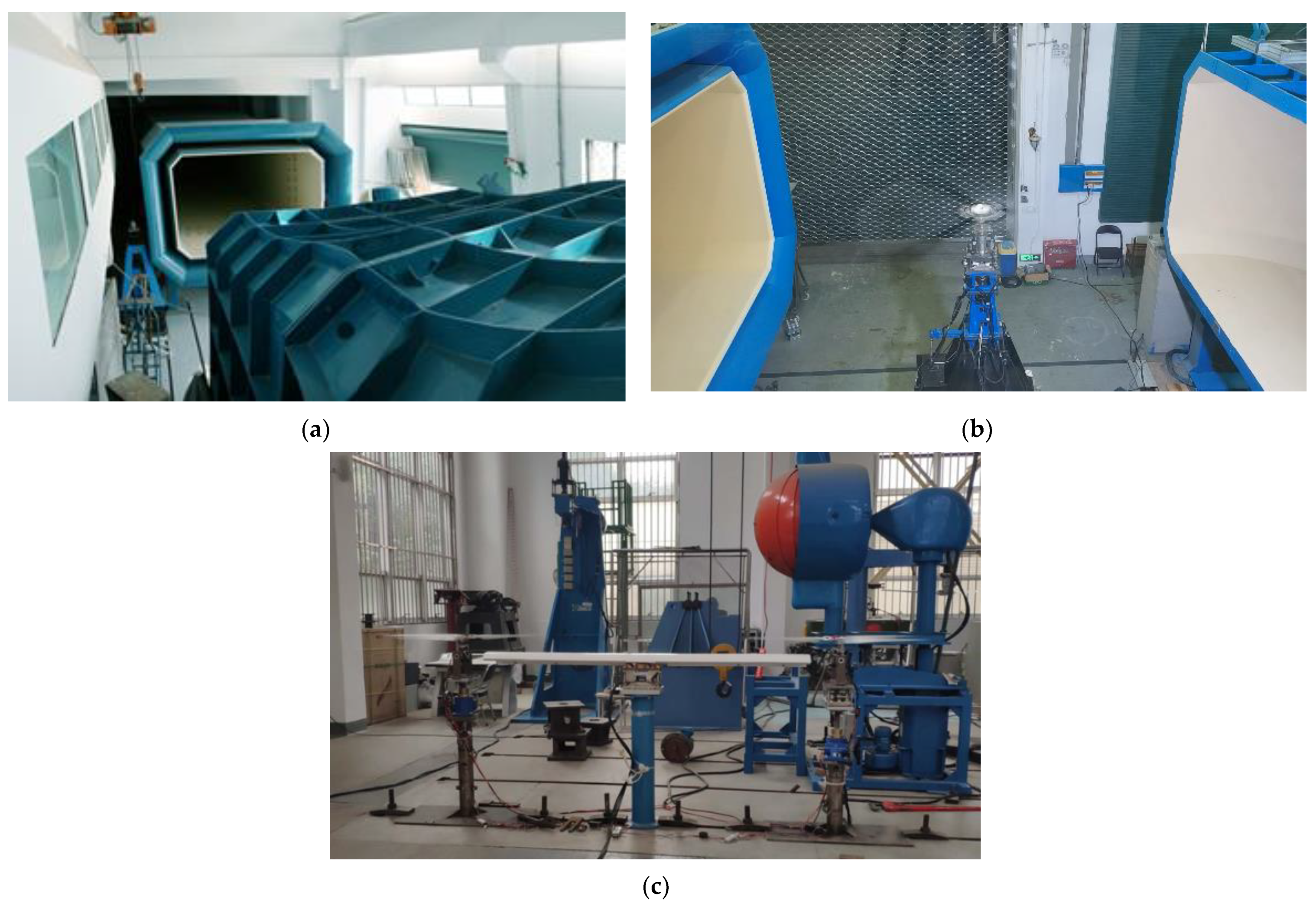
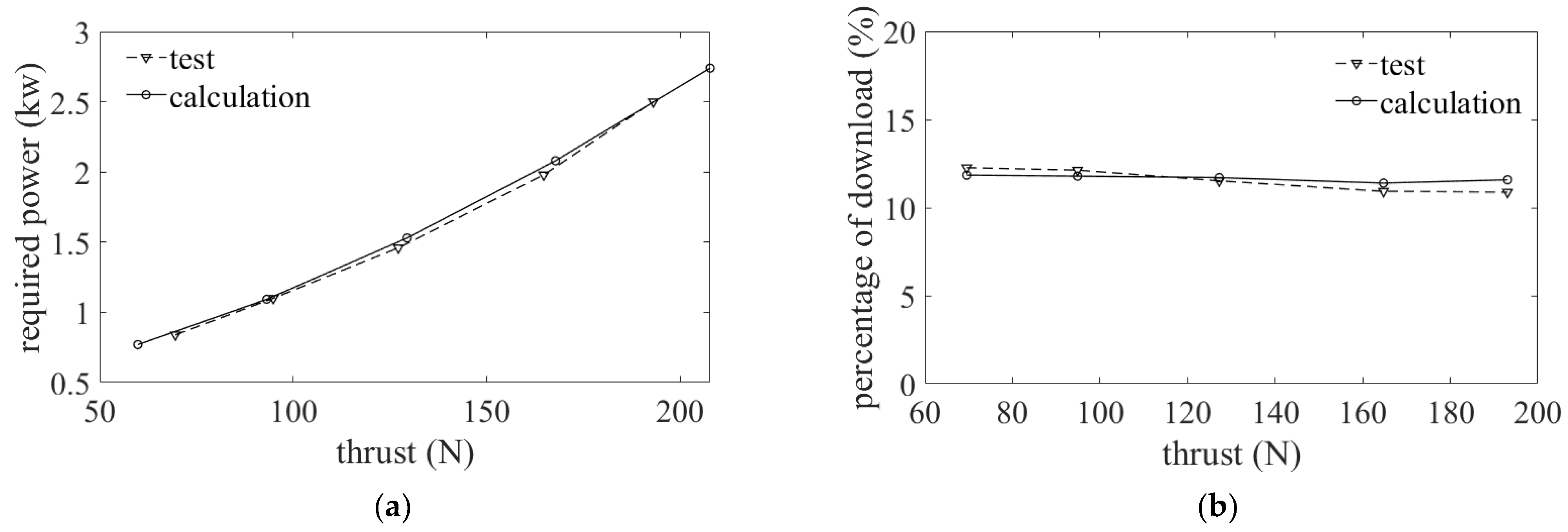
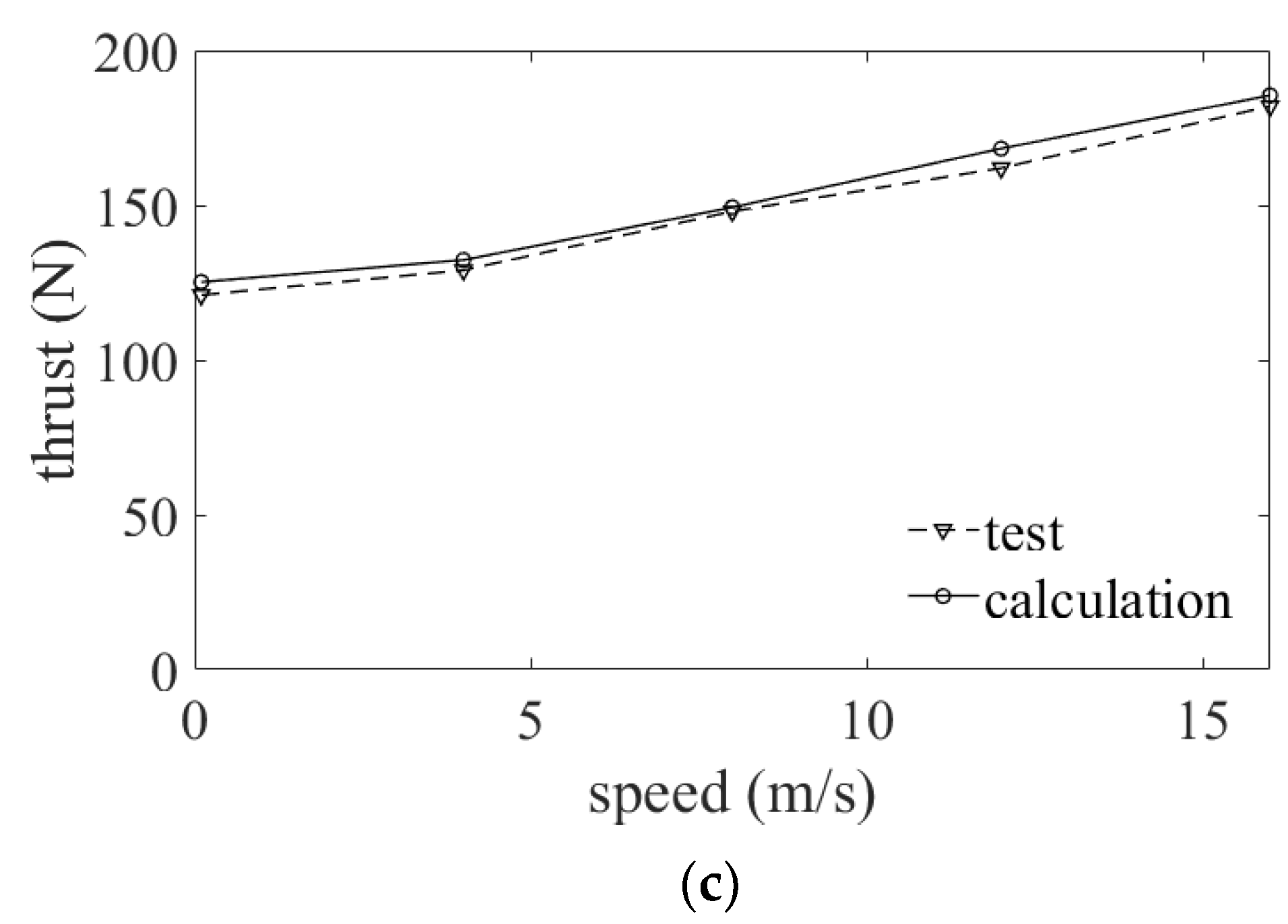
2.5. Validation
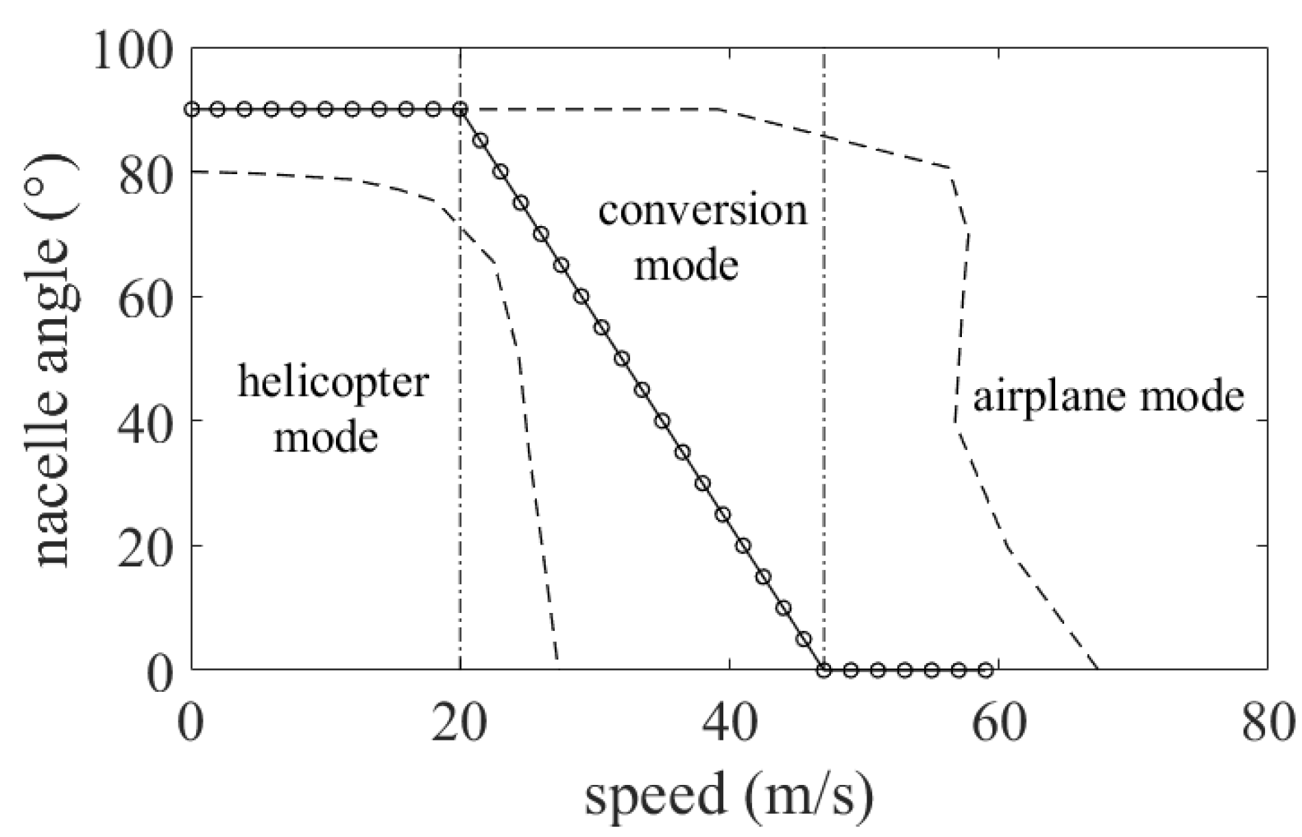
3. Control Strategy
3.1. Strategy in the Helicopter Mode
3.2. Strategy in the Airplane Mode
4. Results
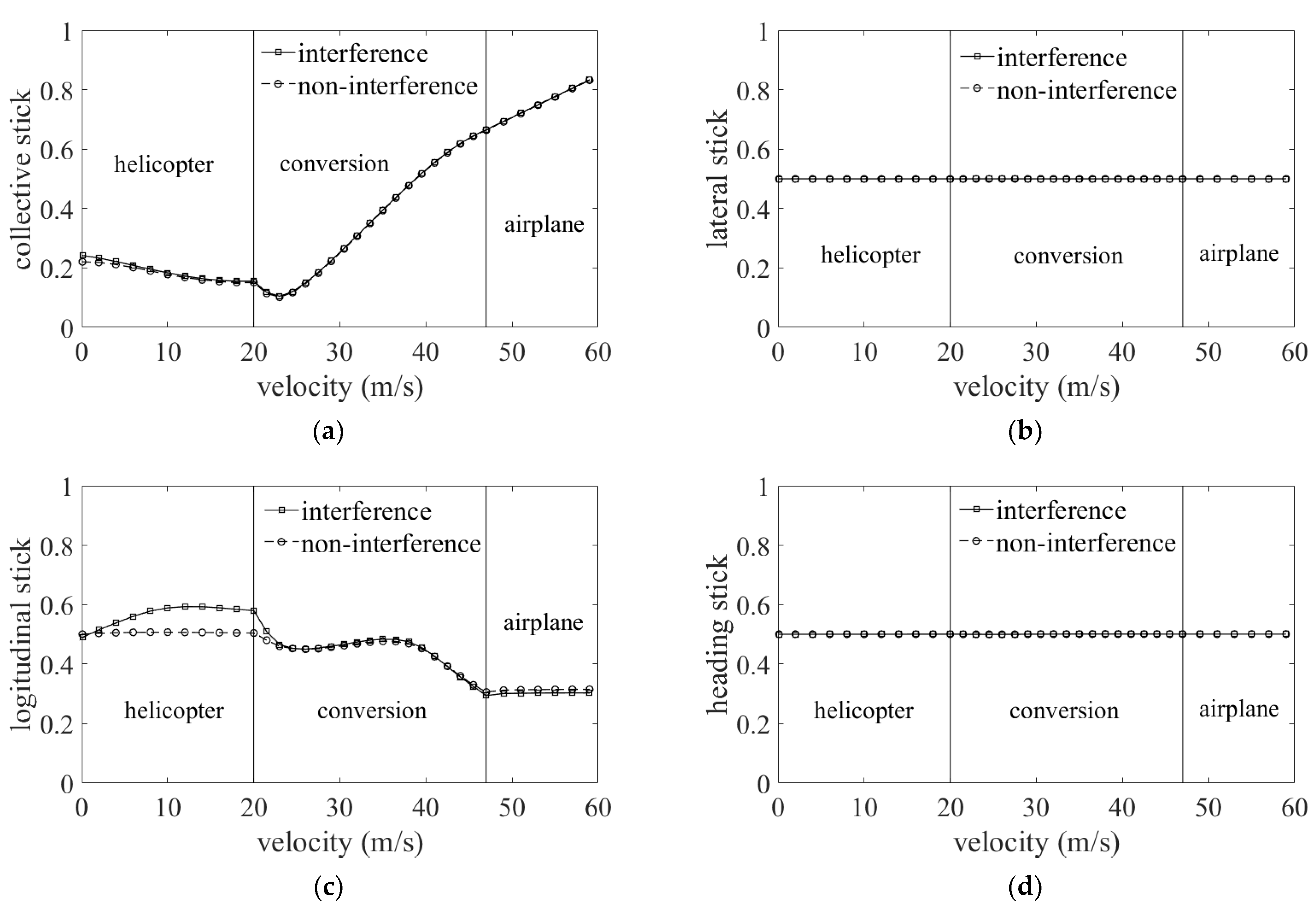
4.1. Influence on Displacement of Collective Stick
4.2. Influence on Longitudinal Trim Characteristic
5. Conclusions
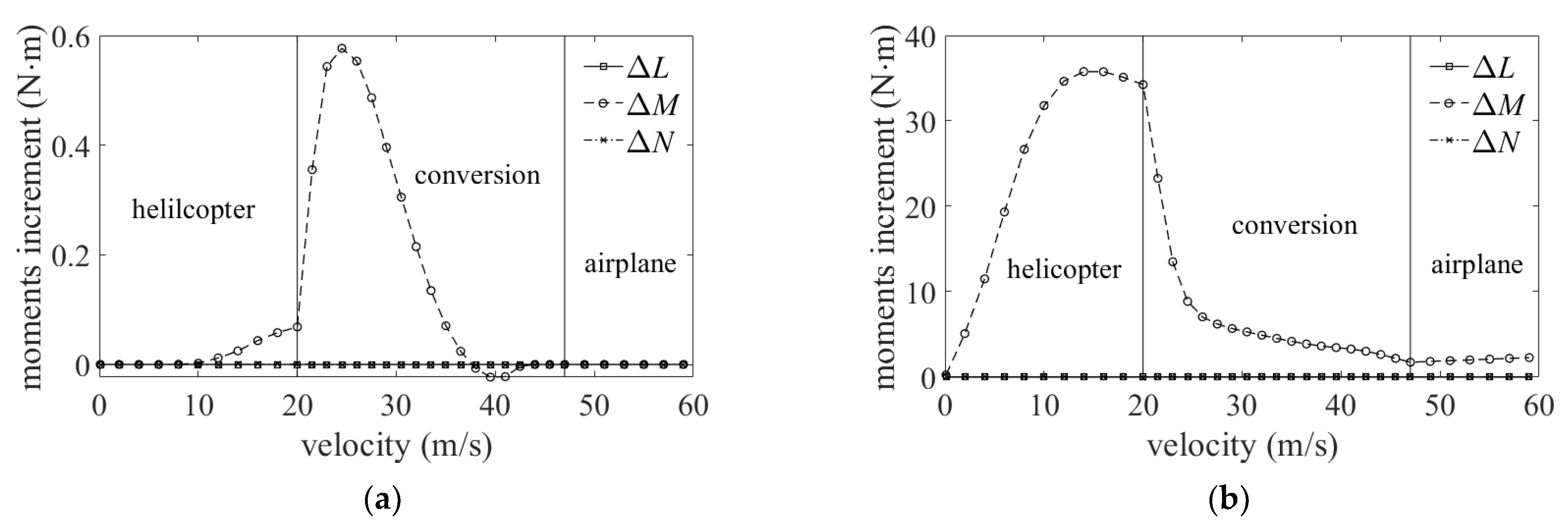
- The interference of lateral rotor–rotor has little influence on the body forces and moments. The maximum variation of the vertical force increment is 13 N, which accounts for 2.2% of the vehicle’s weight. On the other hand, the interference of the longitudinal rotor–rotor mainly affects the vertical force and pitching moment. The maximum vertical force increment is 21 N, which accounts for 3.6% of the overall weight. In addition, the nose-up pitching moment varies greatly, with a maximum value of 36 N∙m;
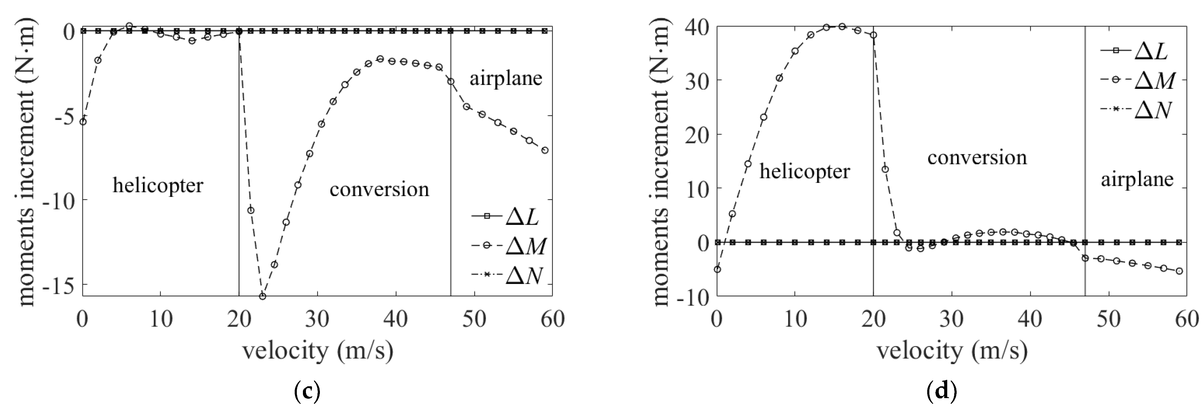
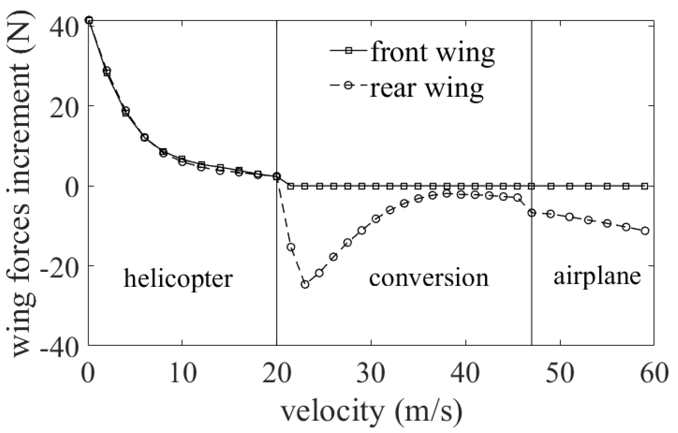
- The interference of the rotor–wing mainly affects the vertical force and pitching moment. The variation of the vertical force increment reaches its maximum in the hover state, accounting for 13.6% of the vehicle’s weight. At this time, a nose-down pitching moment of about 5 N∙m will be generated. The pitching moment will be changed significantly in the conversion mode, and the corresponding maximum pitching moment is 15 N∙m.
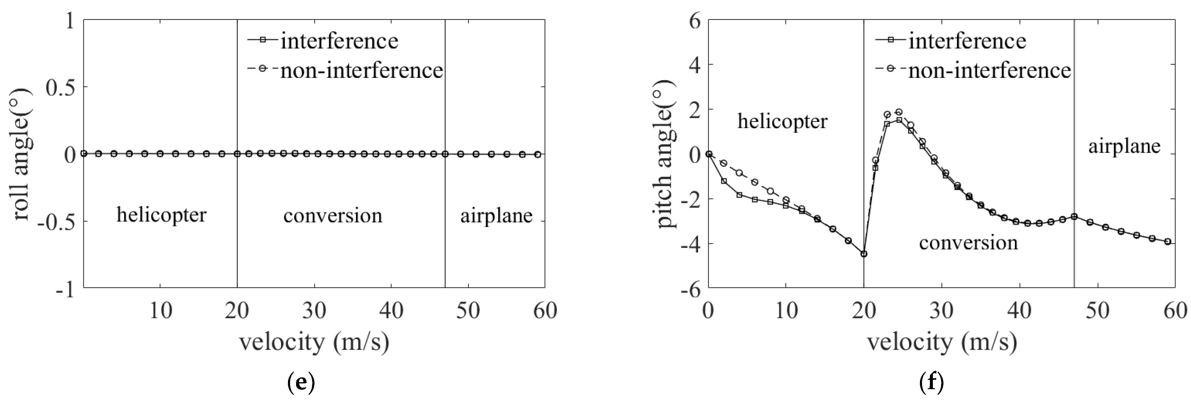
- The trim values of the longitudinal stick and the pitching angle are affected significantly by rotor–rotor and rotor–wing interference in the helicopter mode and conversion mode with a lower tilt angle. The interaction also affects the longitudinal stick in the airplane mode and the collective stick at low-speed range in the helicopter mode.
Author Contributions
Funding
Institutional Review Board Statement
Informed Consent Statement
Data Availability Statement
Conflicts of Interest
References
- Braganca, E. The V-22 Osprey: From Troubled Past to Viable and Flexible Option. Jt. Force Q. 2012, 66, 80–84. [Google Scholar]
- King, D. A System Engineering Approach to Carefree Maneuvering in The BA609. In Proceedings of the American Helicopter Society 61st Annual Forum, Grapevine, TX, USA, 1–3 June 2005. [Google Scholar]
- Snyder, D. The Quad Tiltrotor: Its Beginning and Evolution. In Proceedings of the International Powered Lift Conference, Arlington, VA, USA, 30 October–1 November 2000. [Google Scholar]
- Marr, R.; Blackman, S.; Weiberg, J.; Schroers, L.G. Wind tunnel and flight test of the XV-15 Tilt Rotor Research Aircraft. In Proceedings of the 35th Annual National Forum, Washington, DC, USA, 21–23 May 1979. [Google Scholar]
- Radhakrishman, A.; Schmitz, F. Quad Tilt Rotor Aerodynamics in Ground Effect. In Proceedings of the AIAA Applied Aerodynamics Conference, Toronto, ON, Canada, 5–8 June 2006. [Google Scholar]
- Muraoka, K.; Okada, N.; Kubo, D. Quad Tilt Wing VTOL UAV: Aerodynamics Characteristics and Prototype Flight Test. In Proceedings of the Aerospace Conference, Seattle, WA, USA, 7–14 March 2009. [Google Scholar]
- Yuan, Y.; Chen, R.; Li, P. Trim investigation for coaxial rigid rotor helicopters using an improved aerodynamic interference model. Aerosp. Sci. Technol. 2019, 85, 293–304. [Google Scholar] [CrossRef]
- Ji, H.; Chen, R.; Lu, L.; White, M.D. Pilot workload investigation for rotorcraft operation in low-altitude atmospheric turbulence. Aerosp. Sci. Technol. 2021, 111, 106567. [Google Scholar] [CrossRef]
- Li, P.; Chen, R. A Mathematical Model for Helicopter Comprehensive Analysis. Chin. J. Aeronaut. 2010, 23, 320–326. [Google Scholar]
- Sheng, C.; Narramore, C.J. Computational Simulation and Analysis of Bell Boing Quad Tiltrotor Aero Interaction. J. Am. Helicopter Soc. 2009, 54, 42002. [Google Scholar] [CrossRef]
- Patrick, P.; Andreas, K.; Damien, D.; Breitsamter, C. Numerical Investigation of an Optimized Rotor Head Fairing for the RACER Compound Helicopter in Cruise Flight. Aerospace 2021, 8, 66. [Google Scholar]
- Shi, Y.; Li, G.; Su, D.; Xu, G. Numerical Investigation on ship/multi-helicopter dynamic interface. Aerosp. Sci. Technol. 2020, 106, 106175. [Google Scholar] [CrossRef]
- Ferguson, S. A Mathematical Model for Real Time Flight Simulation of a Generic Tilt-Rotor Aircraft; NASA CR-166536; NASA: Washington, DC, USA, 1988. [Google Scholar]
- Ostroff, J.; Downing, D.; Rood, W. A Technique Using a Nonlinear Helicopter Model for Determining Trims and Derivatives; NASA Technical Note D-8159; NASA: Washington, DC, USA, 1976. [Google Scholar]
- Johnson, W. Influence of Lift Offset on Rotorcraft Performance; NASA/TP-2009-215404; NASA: Washington, DC, USA, 2009. [Google Scholar]
- Yan, X.; Chen, R. Control strategy optimization of dynamic conversion procedure of tiltrotor aircraft. Acta Aeronaut. Astronatica Sinca 2017, 38, 520865. [Google Scholar]
- Wang, Z.; Li, J.; Duan, D. Manipulation Strategy of Tilt Quad Rotor Based on Active Disturbance Rejection Control. J. Aerosp. Eng. 2020, 234, 573–584. [Google Scholar] [CrossRef]
- Talbot, P.; Tinling, B.; Decker, W. A Mathematical Model of a Single Main Rotor Helicopter for Piloted Simulation; NASA Technical Memorandum 84281; NASA: Washington, DC, USA, 1982. [Google Scholar]
- Chen, R. A Simplified Rotor System Mathematical Model for Piloted Flight Dynamics Simulation; NASA Technical Memorandum 78575; NASA: Washington, DC, USA, 1979. [Google Scholar]
- McCroskey, W.; Spalart, P.; Laub, G.; Maisel, M.; Maskew, B. Air Loads on Bluff Bodies, with Application to the Rotor-Induced Downloads on Tiltrotor Aircraft; NASA-TM-84401; NASA: Washington, DC, USA, 1983. [Google Scholar]
- Carlson, E.; Zhao, Y. Optimal short takeoff of tiltrotor aircraft in one engine failure. J. Aircr. 2002, 39, 280–289. [Google Scholar] [CrossRef]
- Wang, J.; Yu, Z.; Chen, R.; Wang, Z.; Lu, J. Aerodynamic characteristics of quad tilt rotor aircraft in vertical flight. J. Aerosp. Power 2021, 36, 249–263. [Google Scholar]
- Ji, H.; Chen, R.; Li, P. Real-time simulation model for helicopter flight task analysis in turbulent atmospheric environment. Aerosp. Sci. Technol. 2019, 92, 289–299. [Google Scholar] [CrossRef]
- Maisel, M. The History of the XV-15 Tilt Rotor Research Aircraft from Concept to Flight; NASA SP-2000-4517; NASA: Washington, DC, USA, 2000. [Google Scholar]


| Parameters | Values | Parameters | Values |
|---|---|---|---|
| gross weight/kg | 60 | rotor solidity ratio | 0.0938 |
| rotor rotational speed/rpm | 2100 | motor valuable power for rotors/kw | 4.8 × 4 |
| number of blades | 3 | mean chord of wing/m | 0.3 |
| rotor radius/m | 0.58 | distance between front and rear wings/m | 1.2 |
| blade chord/m | 0.057 | fuselage length/m | 2 |
| front wing span/m | 1.6 | fuselage width/m | 2.6 |
| rear wing span/m | 2.2 | fuselage height/m | 0.5 |
| Rotor Number | 1 | 2 | 3 | 4 |
|---|---|---|---|---|
| 1 | — | Lateral | — | Longitudinal |
| 2 | Lateral | — | Longitudinal | — |
| 3 | — | Longitudinal | — | Lateral |
| 4 | Longitudinal | — | Lateral | — |
| Components | Control Surface | Number |
|---|---|---|
| Rotor | Collective | 3 × 4 = 12 |
| Longitudinal cyclic | ||
| Lateral cyclic | ||
| Wing | Flaperon | 2 × 2 = 4 |
| Empennage | Rudder | 1 |
| Control | Rotor 1 | Rotor 2 | Rotor 3 | Rotor 4 |
|---|---|---|---|---|
| Collective | ||||
| Longitudinal cyclic | 0 | 0 | 0 | 0 |
| Lateral cyclic |
Publisher’s Note: MDPI stays neutral with regard to jurisdictional claims in published maps and institutional affiliations. |
© 2022 by the authors. Licensee MDPI, Basel, Switzerland. This article is an open access article distributed under the terms and conditions of the Creative Commons Attribution (CC BY) license (https://creativecommons.org/licenses/by/4.0/).
Share and Cite
Zhou, P.; Chen, R.; Yuan, Y.; Chi, C. Aerodynamic Interference on Trim Characteristics of Quad-Tiltrotor Aircraft. Aerospace 2022, 9, 262. https://doi.org/10.3390/aerospace9050262
Zhou P, Chen R, Yuan Y, Chi C. Aerodynamic Interference on Trim Characteristics of Quad-Tiltrotor Aircraft. Aerospace. 2022; 9(5):262. https://doi.org/10.3390/aerospace9050262
Chicago/Turabian StyleZhou, Pan, Renliang Chen, Ye Yuan, and Cheng Chi. 2022. "Aerodynamic Interference on Trim Characteristics of Quad-Tiltrotor Aircraft" Aerospace 9, no. 5: 262. https://doi.org/10.3390/aerospace9050262
APA StyleZhou, P., Chen, R., Yuan, Y., & Chi, C. (2022). Aerodynamic Interference on Trim Characteristics of Quad-Tiltrotor Aircraft. Aerospace, 9(5), 262. https://doi.org/10.3390/aerospace9050262