Numerical Simulation of Tiltrotor Flow Field during Shipboard Take-Off and Landing Based on CFD-CSD Coupling

Abstract

Due to the small tilt angle, a tiltrotor operates in non-axial flow conditions during shipboard take-off and landing. The non-uniformity of the blade’s air-load is high, resulting in structural deformation with high fluctuation frequency, affecting the rotor’s aerodynamic characteristics. A new computational fluid-dynamic computational structural dynamics (CFD-CSD) solver is proposed to analyze the effects of the blade’s elastic deformation on the aerodynamic characteristics. This method is suitable for the aeroelastic simulation of shipboard tiltrotor take-offs and landings. The CFD method uses the Reynolds-averaged Navier-Stokes (RANS) equations as the control equation, while the CSD solver is based on the Timoshenko beam model. The solvers are combined with a two-way loose coupling strategy to improve the solution efficiency. The reverse overset assembly technique (ROAT) is utilized to eliminate the effects of orphan mesh points after deformation. The simulation is conducted during take-off and landing at different heights and different tilt angles, using the XV-15 tiltrotor as an example. An analysis of the rotor’s air-load and the mutual interference of the vortex and wake indicates that when the tiltrotor takes off or lands with a small tilt angle, the wing shedding vortex causes the rotor’s wake to roll upward before it reaches the ship’s deck, producing strong thrust fluctuations. The elastic deformation of the blade reduces the fluctuations in the thrust amplitude. This phenomenon is more pronounced in areas of high fluctuations in the blade’s air-load.

1. Introduction

Shipboard tiltrotor take-offs and landings are high-risk flight maneuvers. Due to the turbulence interference caused by the sea wind blowing through the wing, the flow field environment of a tiltrotor is complex during take-off and landing. The tilt state also affects the flow field. Therefore, it is essential to investigate the shipboard take-off and landing flow field of tiltrotors. The blades are sensitive to flow changes due to their elasticity, resulting in a coupling problem of aerodynamic forces and structural elasticity. When the blades rotate under these conditions, the blade tips are prone to flapping excessively and can potentially collide with the fuselage, leading to serious safety problems [1]. Therefore, we develop a coupled computational fluid-dynamic-computational structural dynamics (CFD-CSD) solver to simulate the flow field of a tiltrotor during shipboard take-off and landing.

Shipboard take-offs and landings by a tiltrotor can be regarded as low-speed near-ground flight maneuvers. Researchers have investigated near-ground flight, take-off, and landing by helicopters using simulations and theoretical analyses. Many studies used the free-wake method [2,3,4]. Kang and Sun [4] used this method to calculate the flow field of bi-rotor aircraft, to determine the shape of the wake during near-ground flight. However, it is difficult to simulate the flow field of a tiltrotor during shipboard take-off and landing using the wake model. After CFD methods became more popular in rotor aerodynamic studies, more accurate rotor wakes and blade air-loads were simulated. Hwang et al. [5] used an unstructured overset mesh method to study the ground effect of different rotors to predict the vortex structure and wake shape more accurately. Lakshminarayan et al. [6] performed detailed simulations of the vortex nucleus positions and downwash velocities at different heights. The results provided a good match with the test points. Young [7] used CFD to calculate the aerodynamic characteristics of tiltrotors approaching a building during near-ground flight, to study the changes in the aerodynamic environment. However, few studies have been conducted on near-ground flights of tiltrotors, especially numerical simulations that consider the tiltrotor’s take-off and landing flow field.

Since tiltrotors have wings, their aerodynamic characteristics differ from those of helicopter rotors. Potsdam et al. [8] and Ye et al. [9] investigated tiltrotor/wing interactions during hovering and demonstrated that the blade air-load was higher at the position where the blade rotated above the wing. At this position, the wing was affected by the rotor’s downwash flow, and the maximum load occurred below the inside area of the rotor. However, these studies did not investigate forward flight. The effect of the wing during shipboard take-off and landing depends on the direction of the incoming flow, which is much more complex than during hovering far from the ground. Therefore, we simulate the flow field when the rotor is tilted forward/backward at different angles. The results show that the area of the blade air-load caused by the wing effect is closely related to the tilt angle. The blade air-load is more uneven when the rotor is tilted backward, due to the strong influence of the wing vortex generated by the sea wind in the rotor’s wake. At this time, the periodic fluctuations of the blade’s deformation due to its elasticity are stronger, and the effect on the aerodynamic characteristics is more pronounced.

A new CFD-CSD coupling solver suitable for simulating the flow field of the rotor is established herein. This model is based on previous studies by our research group [10,11,12,13,14]. It integrates solvers for two domains (aerodynamics and solid structural mechanisms). The blade deformation obtained from the CSD model is simulated in the CFD model using sectional mesh motion to perform the flow field simulation and aerodynamic calculations, based on an elastic blade model.

The CFD-CSD method can yield a better result than the CFD method for calculating the rotor flow field [15,16,17]. Min et al. [18] analyzed the vibration reduction of Hart-II blades using CFD-CSD loose coupling. Lim [19] utilized the rotor aerodynamic calculation software OVERFLOW2 and CAMRAD-II to determine the structural mechanism and optimize the blade performance. Khawar et al. [20] utilized commercial codes to perform the CFD-CSD calculation for fixed wings, in which study the CSD solver is based on finite element software. Compared with the finite-beam model, the finite element method takes much more time to source the deformation data. In this study, the finite-beam model CSD solver is coupled with a CFD solver based on a loose coupling strategy, which can utilize the quasi-steady state of rotor flow to reduce the computational time. Jung et al. [21] modeled the wing based on the Euler–Bernoulli beam, which supposes that the deformed section is vertical to the elastic axis. The Timoshenko beam model used in this study does not take that assumption and allows that the shearing deformation exists on sections; this results in a more accurate deformation than the Euler–Bernoulli beam model. Goulos et al. [22] performed an aeroelastic analysis of rotor-fuselage interaction, while the air load was calculated using a finite-state inflow model, with which it is difficult to simulate the flow field of the rotor after deformation. Wang et al. [23] also analyzed the rotor-fuselage aeroelasticity and used the dynamic mesh method to realize the blade elastic deformation. However, the CFD solver used in their research is based on Eulerian equations. It does not take the fluid viscosity into account, while the Reynolds-averaged Navier–Stokes (RANS) equations can achieve this with the turbulence model added. A loose coupled CFD-CSD solver, developed by the authors, is used in the current study. The CSD solver is based on the Timoshenko beam model, and the CFD solver uses the RANS equations. After the elastic deformation of the blade mesh has been obtained, the overset mesh system must ensure accurate interpolation between meshes. The reverse overset assembly technique (ROAT) [11] developed previously by the author is used to construct the overset mesh system to deal with the conservative variable interpolation after the deformation of the blade mesh, prevent orphan mesh points, and improve the robustness of the deformed mesh.

The results show that the proposed CFD-CSD method results in a lower amplitude of the thrust fluctuation in one revolution than the CFD method, and the elastic deformation reduces the amplitude of the thrust fluctuation caused by the wing’s vortex interference in a backward tilt scenario.

2. Numerical Simulation Method

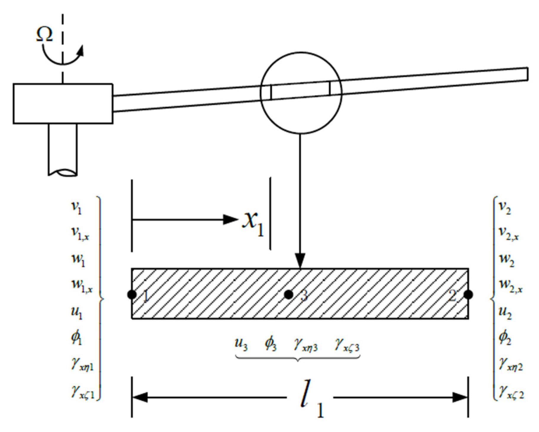
2.1. CFD and CSD Numerical Solvers

The CFD solver is developed by the authors. It uses the RANS equations [14] as governing equations to solve the flow filed in the air domain:

$$\frac{\partial }{\partial t}{\displaystyle {\iiint }_V\overrightarrow{W}}dV+{\displaystyle {\iint }_{\partial V}\overrightarrow{F_c}}\cdot \overrightarrow{n}dS-{\displaystyle {\iint }_{\partial V}\overrightarrow{F_V}}\cdot \overrightarrow{n}dS=0$$

(1)

where

$$\overrightarrow{W}=\left[\begin{array}{c}\rho \\ \rho u\\ \rho v\\ \rho w\\ \rho E\end{array}\right], \overrightarrow{F_c}=\left[\begin{array}{c}\rho \left({\overrightarrow{q}}_n-{\overrightarrow{q}}_b\right)\\ \rho u\left({\overrightarrow{q}}_n-{\overrightarrow{q}}_b\right)+p{\overrightarrow{I}}_x\\ \rho v\left({\overrightarrow{q}}_n-{\overrightarrow{q}}_b\right)+p{\overrightarrow{I}}_y\\ \rho w\left({\overrightarrow{q}}_n-{\overrightarrow{q}}_b\right)+p{\overrightarrow{I}}_z\\ \rho H\left({\overrightarrow{q}}_n-{\overrightarrow{q}}_b\right)+p{\overrightarrow{q}}_b\end{array}\right], \overrightarrow{F_V}=\left[\begin{array}{c}0\\ {\tau }_{xx}{\overrightarrow{I}}_x+{\tau }_{yx}{\overrightarrow{I}}_y+{\tau }_{zx}{\overrightarrow{I}}_z\\ {\tau }_{xy}{\overrightarrow{I}}_x+{\tau }_{yy}{\overrightarrow{I}}_y+{\tau }_{zy}{\overrightarrow{I}}_z\\ {\tau }_{xz}{\overrightarrow{I}}_x+{\tau }_{yz}{\overrightarrow{I}}_y+{\tau }_{zz}{\overrightarrow{I}}_z\\ {\Phi }_x{\overrightarrow{I}}_x+{\Phi }_y{\overrightarrow{I}}_y+{\Phi }_z{\overrightarrow{I}}_z\end{array}\right]$$

(2)

where $\overrightarrow{W}$ represents the vector of the conservative variables; $\overrightarrow{F_C}$ and $\overrightarrow{F_V}$ are the vectors of the inviscid flux and viscous flux, respectively. p, ρ, and E denote the pressure, density, and total energy of the element. u, v, and w are the velocity components in Cartesian coordinates. ${\overrightarrow{q}}_n$ and ${\overrightarrow{q}}_b$ represent the mesh velocity vectors. ${\tau }_{ij}$ are the components of shear stress. A dual mesh paradigm is used in the overset mesh system. The flow field consists of a near-body region and an off-body region. The latter is composed of wake-capture region (refined mesh and close to rotor) and big background (relatively coarse). A Roe scheme is used for spatial discretization of the near-body region (rotor and wing meshes), and the off-body region is discretized with the central scheme. The implicit lower-upper symmetric Gauss-Seidel (LU-SGS) scheme is used for temporal discretization, and the turbulence model is the Spalart-Allmaras model. The ROAT is used for overset mesh interpolation. Figure 1 compares the overset mesh system established with the ROAT and the original criterion provided by Löhner [24]. The ROAT uses a strategy of searching for donor cells before identifying the interpolation boundaries. Empty areas without donor cells can be avoided when selecting the interpolation boundaries, preventing orphan points. The overset mesh system used in the simulation is shown in Figure 2. It is assumed that the take-off and landing area is sufficiently large to disregard the influence of ship buildings on the rotors.

A rotary beam CSD solver is develop by the authors. The beam element model in the CSD calculation is based on the Timoshenko beam [25]. The explicit precise time-integration method [26] is used to obtain the displacement solution corresponding to the blade airload. The blade beam model based on the Timoshenko beam has 20 degrees of freedom, including 4 degrees of freedom of the middle node of the element and 8 degrees of freedom of the nodes at both ends. The degrees of freedom describe the displacement angles $v_i$, $w_i$, the rotation angles $v_{i,x}$, $w_{i,x}$, the torsion displacement ${\varphi }_i$, the tensile displacement $u_i$, and the sectional shear ${\gamma }_{x\eta i}$, ${\gamma }_{x\zeta i}$ of the flap and lag directions, respectively. The degrees of freedom are shown in Figure 3. The following interpolation equation for the Timoshenko beam is used to determine the displacement of the blade:

$$\left[\begin{array}{c}v\\ w\\ \varphi \\ u\\ {\overline{\gamma }}_{x\eta }\\ {\overline{\gamma }}_{x\zeta }\end{array}\right]=\mathrm{Diag}\left[\begin{array}{cccccc}{\left\{{\Phi }_v\right\}}^T\hfill & {\left\{{\Phi }_w\right\}}^T\hfill & {\left\{{\Phi }_{\varphi }\right\}}^T\hfill & {\left\{{\Phi }_u\right\}}^T\hfill & {\left\{{\Phi }_{\eta }\right\}}^T\hfill & {\left\{{\Phi }_{\zeta }\right\}}^T\hfill \end{array}\right]\left[\begin{array}{c}V\\ W\\ \mathit{\varphi }\\ U\\ {\Gamma }_{x\eta }\\ {\Gamma }_{x\zeta }\end{array}\right]$$

(3)

where $\left\{{\Phi }_v\right\},\left\{{\Phi }_w\right\},\left\{{\Phi }_{\varphi }\right\},\left\{{\Phi }_u\right\},\left\{{\Phi }_{\eta }\right\},\left\{{\Phi }_{\zeta }\right\}$ are the spatial interpolation functions relative to the coordinates. The finite element method is used to assemble all elements to obtain the mass, damping, and stiffness matrices of the structure and the vector forces. The second-order linear ordinary differential equation describing the dynamic characteristics of the blade is defined follows:

$$\mathit{M}\ddot{\mathit{q}}+\mathit{C}\dot{\mathit{q}}+\mathit{K}\mathit{q}=\mathit{Q}$$

(4)

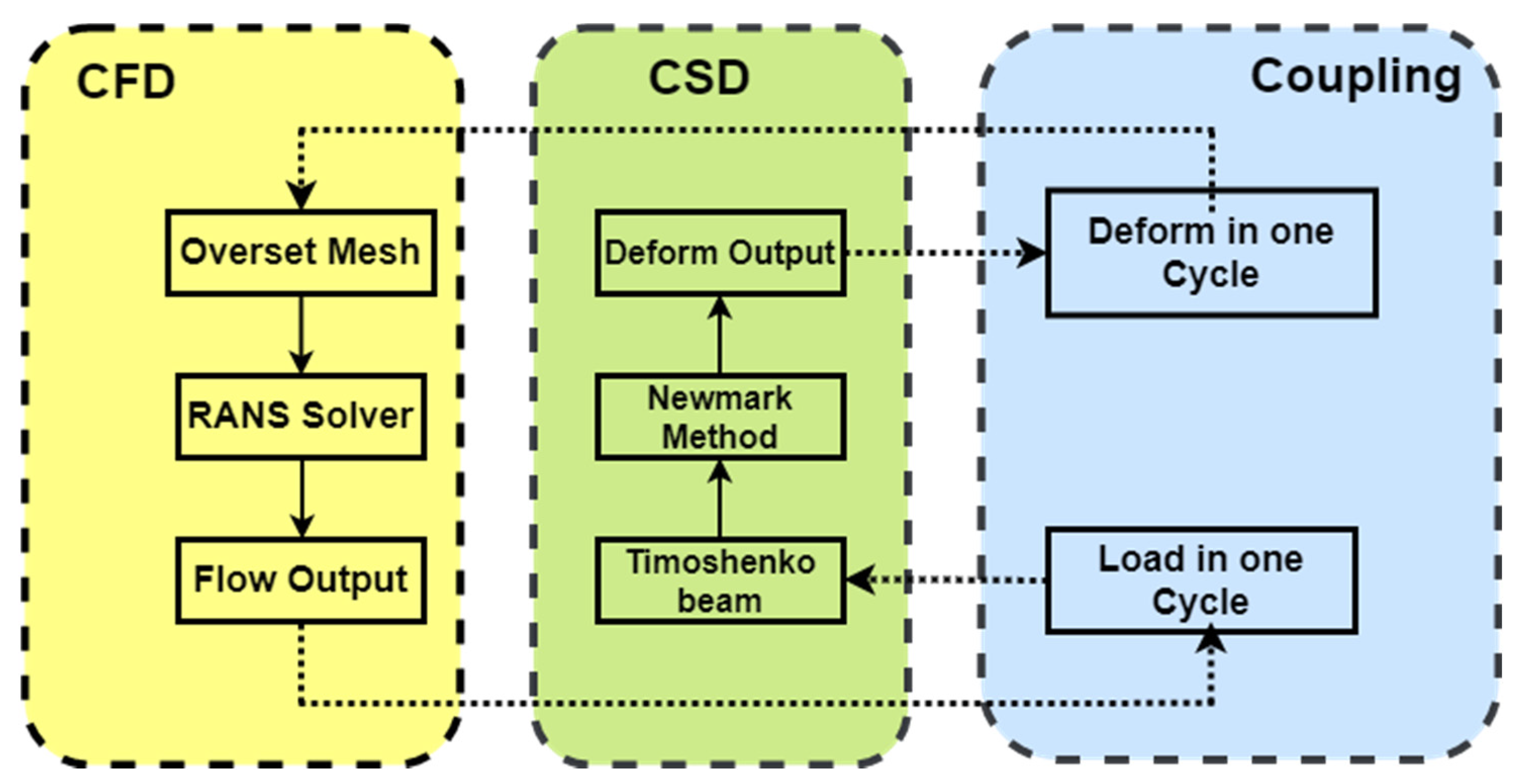
2.2. CFD-CSD Coupling

A loose coupling strategy is used to integrate the CFD and CSD methods [19,27,28] (Figure 4). It consists of three steps: (1) after the initial calculations via CFD, the blade surface pressure of the last revolution is read by the coupling program. The sectional load, such as the sectional tension and torque, is calculated, and the result is input into the CSD program. (2) The CSD program calculates the displacement and torsion angle of the sections according to the sectional load, then the coupling program imports them into the CFD solver. The CFD solver determines the mesh deformation and calculates the blade air-load of a new revolution, according to the imported data. (3) Steps (1) to (2) are repeated until convergence occurs.

3. Verification

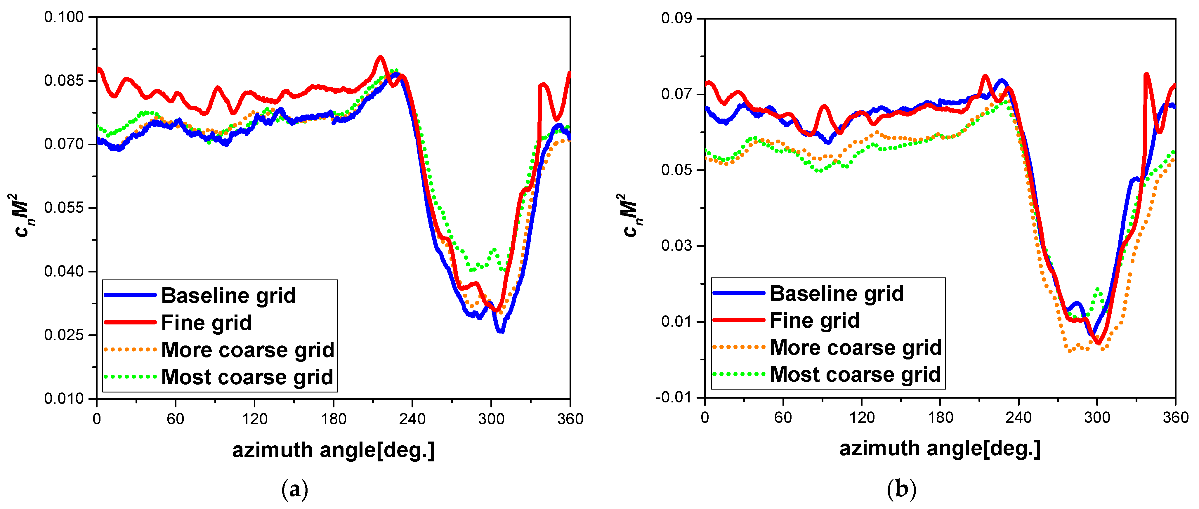
3.1. Grid Independence Verification

The advanced technology blades (ATB) system of the XV-15 tiltrotor [27] is used here. The ATB system consists of three blades with a diameter of 7.62 m and solidity of 0.103. The blade has nonlinear torsion of −47°, an average chord length of 0.411 m, and a square blade tip. The blade shape and airfoil [29] are depicted in Figure 5.

Figure 6 compares the predicted normal force coefficient from four grid systems. The numbers of grid elements are listed in

Table 1. The number of grid elements in the various grid systems for hovering height 1R.

Grid	Blade Mesh	Refined Background	Big Background	Wing	Total Number
Baseline	2,120,398 × 6	4,453,908	1,931,776	1,676,408	10,182,490
Fine	3,865,984 × 6	9,681,424	3,771,264	1,676,408	18,995,080
Coarser	1,716,870 × 6	3,592,092	1,569,152	1,676,408	8,554,521
Coarsest	1,273,016 × 6	1,802,304	805,504	1,676,408	5,557,231

. The hovering height of the rotors is 1R, and the blade tip Mach number M_tip = 0.65. The results from the baseline grid and fine grid compare well with each other. For the 0.85R section, the data of the baseline grid are smaller than that of the fine grid at the interval where the curve varies slightly. However, the valley values of the baseline grid are similar to the fine grid, while the values from the coarse grid systems are largely different from that of the fine grid system. For the purpose of the present work, the primary impact (the range of azimuth angle where the normal force varies sharply) is adequately captured by the baseline grid. Thus, the baseline grid system is used in all simulations.

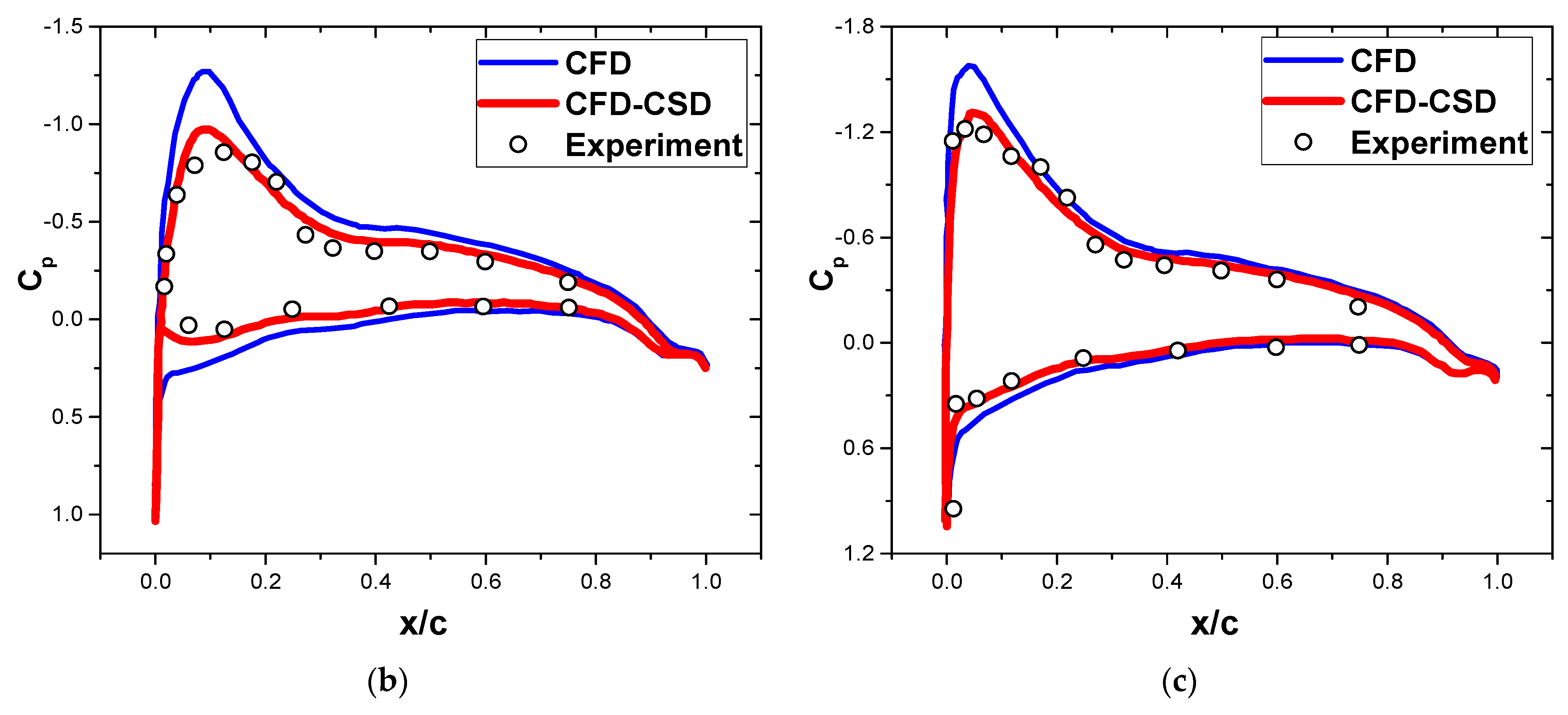
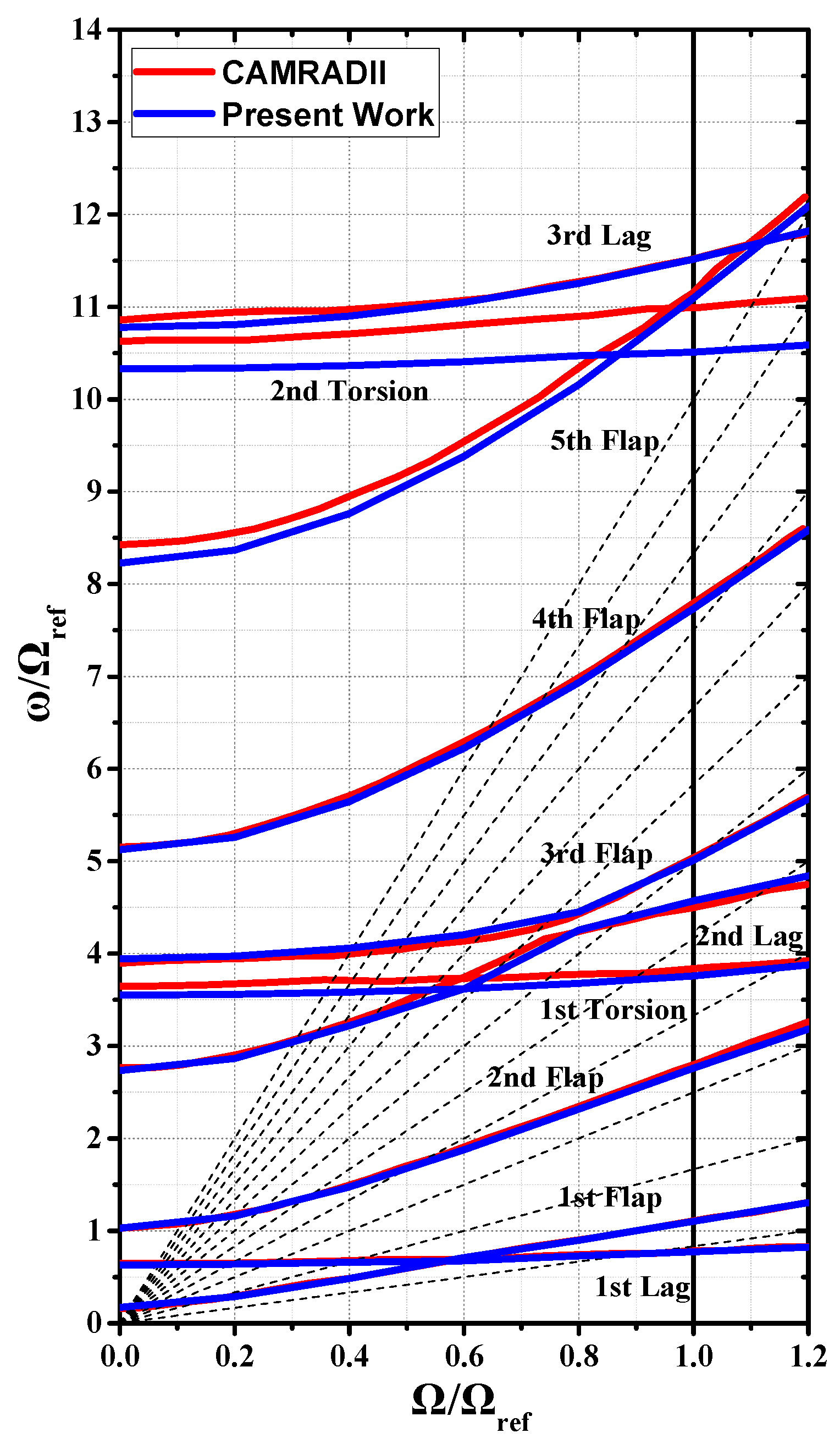
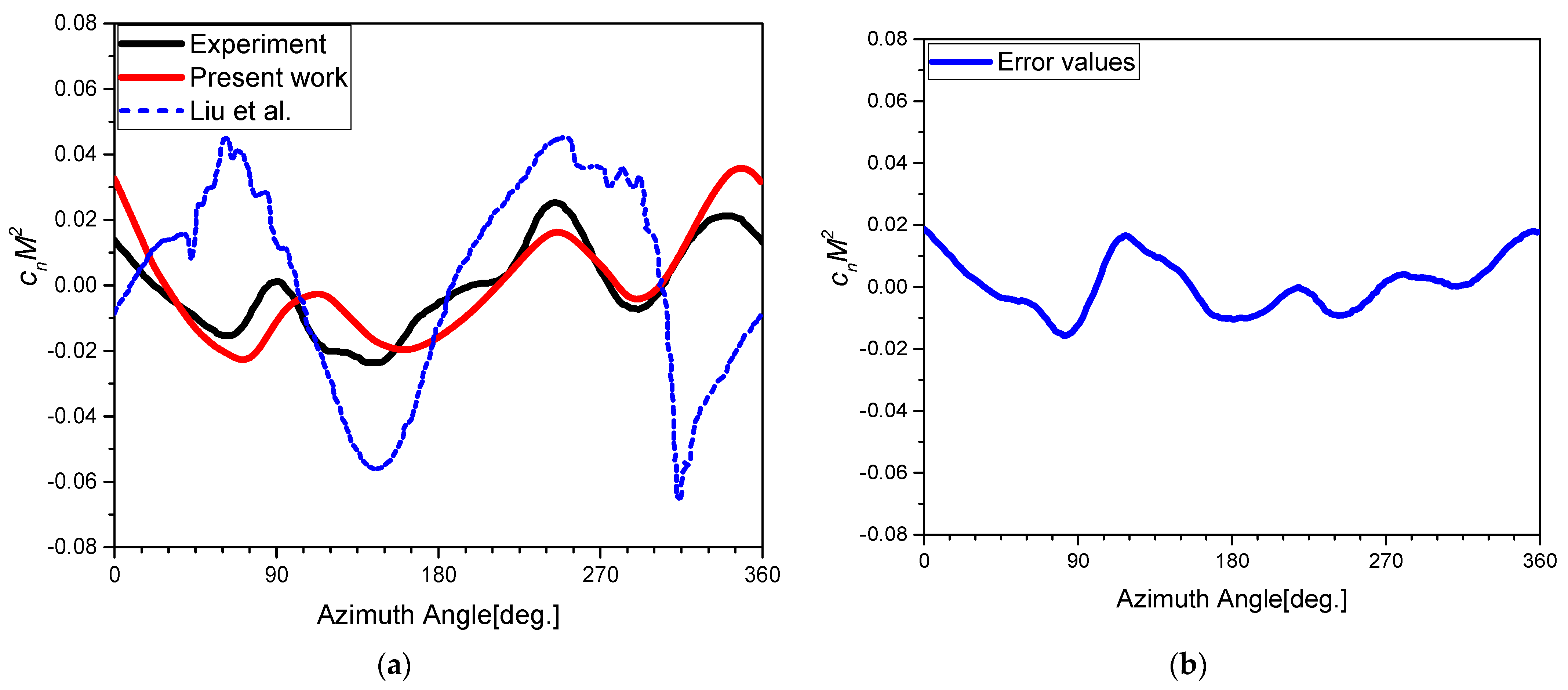
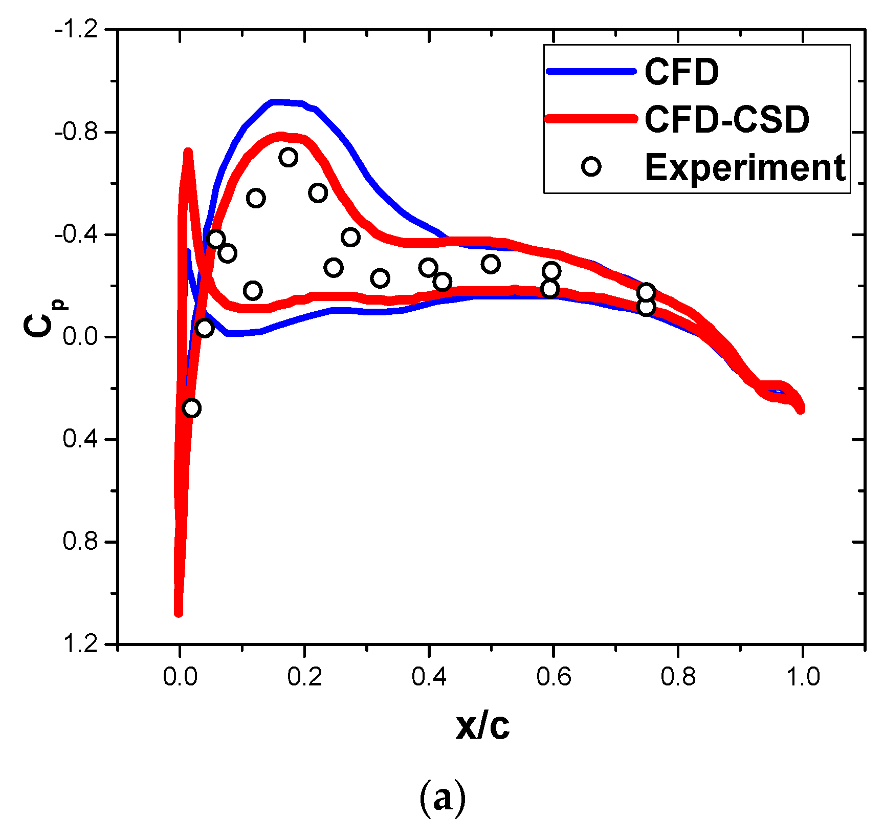
3.2. Verification of the CFD-CSD Coupling Method

The forward flight [30] of the Hart-II rotor is used as an example to verify the effectiveness of the proposed CFD-CSD coupling method. The model rotor has 4 hinged Bo-105 blades with a radius of 2 m and a chord length of 0.121 m. The NACA13012 airfoil, with a linear twist of −8° and a hub pre-cone angle of 2.5°, is used.

Figure 7 provides the calculation results of the blade’s structural characteristics obtained from the proposed method and CAMRAD II [31]. CAMRAD II is a famous rotor structural dynamic software developed by Dr. Wayne Johnson. It has been proved many times to be accurate in calculating the rotor frequency diagram. The results of the present work are in good agreement with the CAMRAD II results, which illustrates the validity of the CSD solver used in this study. Figure 8a shows a comparison of the calculations in the present work, the CFD/CSD/PVTM results by Liu et al. [32], and the experimental results [30] of the normal force coefficient in the 0.87R section. An advance ratio μ of 0.151 and M_tip of 0.639 are considered. The calculated data were obtained after 10 revolutions; the mean was removed, and the high-frequency content was filtered out. The experimental data do not reflect the blade vortex interaction. The vortex effect on the blade might cause unstable high-frequency values, while the experiment filtered the high-frequency content. For the validation used in this study, the same measure is introduced. The results of the coupling method are consistent with the experimental data, and the error is smaller than that of Liu et al. From Figure 8a and the error values between experiment and calculation (Figure 8b), it can be seen that the calculated values are slightly larger on the retreating side. On the retreating side, where a serious stall exists, the CFD solver considers the reverse flow and the low dynamic pressure, resulting in a difference between the calculated and the experimental values. Figure 9 shows the iso-surface of the Q-criterion, calculated by the CFD-CSD coupling method, to visualize the rotor wake. It can be seen from the figure that the CFD-CSD solver in this study can capture the wake of the rotor well. Although numerical diffusion exists, the solver can give the wake structure for at least 5 revolutions.

The pressure coefficient of the Helishape 7A rotor is calculated with the CFD-CSD coupling method to illustrate the utility of this method. The parameter values are M_tip = 0.656 and μ = 0.4. Figure 10 shows the pressure coefficients obtained from the CFD and CFD-CSD methods and the experimental data [16,33] of the 0.975R section on the rotor’s front and side. The azimuth angle of 0° is defined at the rear of the rotor, and it increases with the direction of the rotor. The data of $\psi =180°$ concerns the front and the others concern the side of the rotor. Since the proposed method considers the effect of deformation on the aerodynamic characteristics of the blade, its results are closer to the experimental data than that of the CFD method, and the calculation accuracy is high. In this scenario, the rotor operates at high speed and with an advance ratio close to the general working state of the tiltrotor. Due to a lack of sufficient experimental data on the XV-15 tiltrotor, the coupling method is necessary to study the aerodynamic characteristics of the rotor at high rotation speeds.

4. Results

4.1. Rotor Flow Field When the Ship Is Not Moving

Three cases are evaluated to investigate the influence of the height above the ship’s deck on the aerodynamic characteristics of the rotor: two in-ground effect (IGE) cases with hovering heights of 1R and 2R and one out-of-ground effect (OGE) case which equals to infinite height. The two rotors are symmetrical; thus, only the right rotor is analyzed. The azimuth angle close to the vertical tail is $\psi =0°$, and that above the wing is approximately $\psi =270°$.

Figure 11 shows the distribution of the rotor thrust at 1R height. The symmetrical centerline of the aircraft is on the left side of the figure, and right below the figure is $\psi =0°$. In Figure 11b (1R height without a wing), the thrust is symmetrical at $\psi =270°\sim 90°$ and $\psi =90°\sim 270°$. However, due to the interaction of the two rotors, a significant change occurs close to the centerline of the fuselage; this phenomenon is observed in other hovering states. In addition, a negative thrust zone occurs at the tip of the rotor. The streamline diagram (Figure 12, the flow travelling along the reverse direction of the x axis) indicates that the upward airflow generated by the fountain flow effect results in unfavorable conditions at the rotor tip. The influence of the fountain flow decreases from the rotor tip to the root and disappears near 0.5R, resulting in a sharp change in the thrust from the middle to the rotor tip at $\psi =270°$.

In addition to a decrease in the thrust near $\psi =270°$, the thrust diagram indicates a low thrust zone on the retreating side. The reason is that the airflow on the advance side is affected by the ship’s deck and cannot disperse downward symmetrically due to the wings. Thus, the airflow merges with the fountain flow, resulting in an expansion of the low thrust area.

The tiltrotor wing increases the rotor thrust above the wing during hovering in the OGE, which has been confirmed by many studies [8,9]. For a tiltrotor, the wing has an equivalent ground effect as rotors. However, the thrust distribution in Figure 11a shows that the influence of the wing is reduced when the height above the ship’s deck is low. The thrust distribution is close to symmetrical distribution, as is the case without wings.

Figure 13 shows the normal force coefficient versus the azimuth angle of the 0.5R, 0.7R, 0.8R, and 0.95R sections at different heights. In the 0.5R section, the normal force coefficient is the largest near the azimuth angle of the wing ($\psi =270°$), but the increase at 1R height is significantly smaller than that of the OGE case. At 1R height, the increase in the thrust resulting from the equivalent ground effect of the wing surpasses the influence of the fountain flow in this section. In the sections close to the blade tip, a drop in the normal force occurs near $\psi =270°$, and the minimum value is observed at about $\psi =300°$. But in the section 0.5R, the normal force increases rather than drops near $\psi =270°$, and the azimuth angle of minimum value in blade tip section is that of maximum value at 0.5R section. It can be concluded that, for sections close to blade tip, the fountain flow is the dominant factor affecting the normal force at azimuth angle of around 270°. The wing’s equivalent ground effect is less pronounced in these areas. For the sections closer to blade root, as mentioned before, the fountain flow effect is less than the blade tip, and the wing’s equivalent ground effect make the normal force increase up to the maximum of the whole revolution.

The impact of blade elasticity is more pronounced on the unstable side, i.e., the zone near the fuselage axis. Figure 14 compares the normal force coefficients obtained from the CFD and coupled CFD-CSD methods. At the minimal thrust position (around $\psi =300°$), the CFD calculation results are substantially different from the coupled CFD-CSD results. The IGE results in greater elastic deformation than the OGE in positions with high thrust fluctuations. It can be seen from the figure that the blade torsion, flap and other elastic deformation will change its aerodynamic performance after being subjected to aerodynamic external force. In general, it will reduce the fluctuation of aerodynamic force, which is more obvious in the 1R height hovering state. At the hovering height of 1R, the blade elasticity effect is the most obvious near $\psi =300°$ of the most unstable aerodynamic environment. The CFD-CSD results after the convergence of multi-revolution coupling iteration show that the elastic deformation will flatten the fluctuation at some angles in this state, so that the aerodynamic variation tends to be flat.

4.2. Rotor Flow Field When the Ship Is Moving

When the tiltrotor is taking off and landing on the ship, it needs to fly with a low tilt angle to overcome the forward/backward incoming flow due to the ship’s movement. Here, the incoming flow speed is set to 15 knots, and take-offs and landings with small forward/backward tilt angles are simulated. The tilt angle is denoted as τ, and a forward tilt angle is considered positive. Figure 15 shows the iso-surface of the Q-criterion and the corresponding streamlines at 0.5R for different scenarios (side view). In the backward tilt scenario, the incoming flow is from the trailing edge of the wing to the leading edge. A wing vortex is generated at the leading edge and develops against the wind toward the trailing edge; then, it contacts with the vortex from the trailing edge and merges with the wake generated by the rotor. However, the vortex generated by the wing’s trailing edge in the forward tilt scenario develops downwind and does not merge with the rotor wake. The nucleus of the position where the vortex rolls up on the ship’s deck is at the equal height of the wing in the backward tilt scenario. When interference occurs due to the shedding vortex from the trailing edge of the wing, the rolling vortex nucleus is not close to the ship’s deck but instead at a height of about 0.25R.

The backward and forward tilt scenarios have different blade air-loads due to the different vorticities. Figure 16 compares the thrust for the different scenarios; the black arrow indicates the direction of the incoming flow. Regardless of whether the rotor is tilted forward or backward, the thrust is always higher downstream, and the center of the incremental zone is vertically above the wing. Combined with the results of the vorticity contours, it is concluded that the equivalent ground effect of the wing and the interference by the wing vortex on the rotor wake have caused this thrust distribution. The wing has a significant impact on the rotor when the tiltrotor takes off and lands with a small tilt angle as the ship is moving.

Figure 17 shows the normal force coefficient versus the azimuth angle in different sections. The variation trends of the normal force are opposite in the forward and backward scenarios, i.e., the peaks in the forward tilt scenarios are the valleys in the backward scenarios and vice versa. Regardless of whether the rotor is tilted forward or backward, the normal force of a smaller tilt angle is higher than that of a larger angle in the 0.5R and 0.7R sections. As the tilt angle increases, the windward area of the rotor increases, resulting in a rise in resistance. However, close to the tip, the trend of the force of the backward tilt differs from the other scenarios. When the rotor is tilted backward, a small period of fluctuations in the normal force occurs around $\psi =360°$. As shown in Figure 15, this is the position where the rotor wake and the wing vortex merge, i.e., the unstable flow field that leads to the fluctuation. Figure 18 shows the difference in the normal force coefficients versus the azimuth angle for the 5° and 10° forward/backward tilt angles in sections 0.5R and 0.8R. In section 0.5R, the curves of the forward and backward tilt scenarios cross, and the amplitude of the fluctuation is much smaller than that at 0.8R. It is only about 1/7 for the backward tilt and about 1/4 for the forward tilt. In section 0.8R, the difference in the coefficients is similar for the backward and forward tilt scenarios, but there is a large peak at around $\psi =308°$.

Figure 19 shows the comparison of the normal force coefficient between the CFD results and coupled CFD-CSD results for a tilt angle of τ = −5°. The results of the range $\psi =300°~360°$ are enlarged. The fluctuations are smaller in the CFD-CSD than in the CFD results. Similar to the scenarios when the ship is not moving, it is easier to observe the influence of the blade elasticity on the aerodynamic calculation in the region where the blade air-load fluctuation frequency is larger. The elastic deformation decreases the amplitude of the normal force coefficient fluctuations at the rotor tip. The aerodynamic forces are external forces for structural dynamic equations and the deformation solutions in the equations vary at the same frequency as the external forces. Where the aerodynamic forces fluctuate with high frequency, the elastic deformation also generates high-frequency fluctuation, which results in a sensitivity to elasticity in these positions. Therefore, the difference is larger in the CFD-CSD results than the CFD results because the latter assumes a rigid blade.

5. Conclusions

The coupled CFD-CSD method and the ROAT were used to simulate the flow field of a tiltrotor during shipboard tiltrotor take-off and landing. The effect of the ship’s deck and the wing and tilt angles of the tiltrotor on the flow field were investigated. The vorticity, force, and flow field were analyzed at different heights and tilt angles. The following conclusions were obtained:

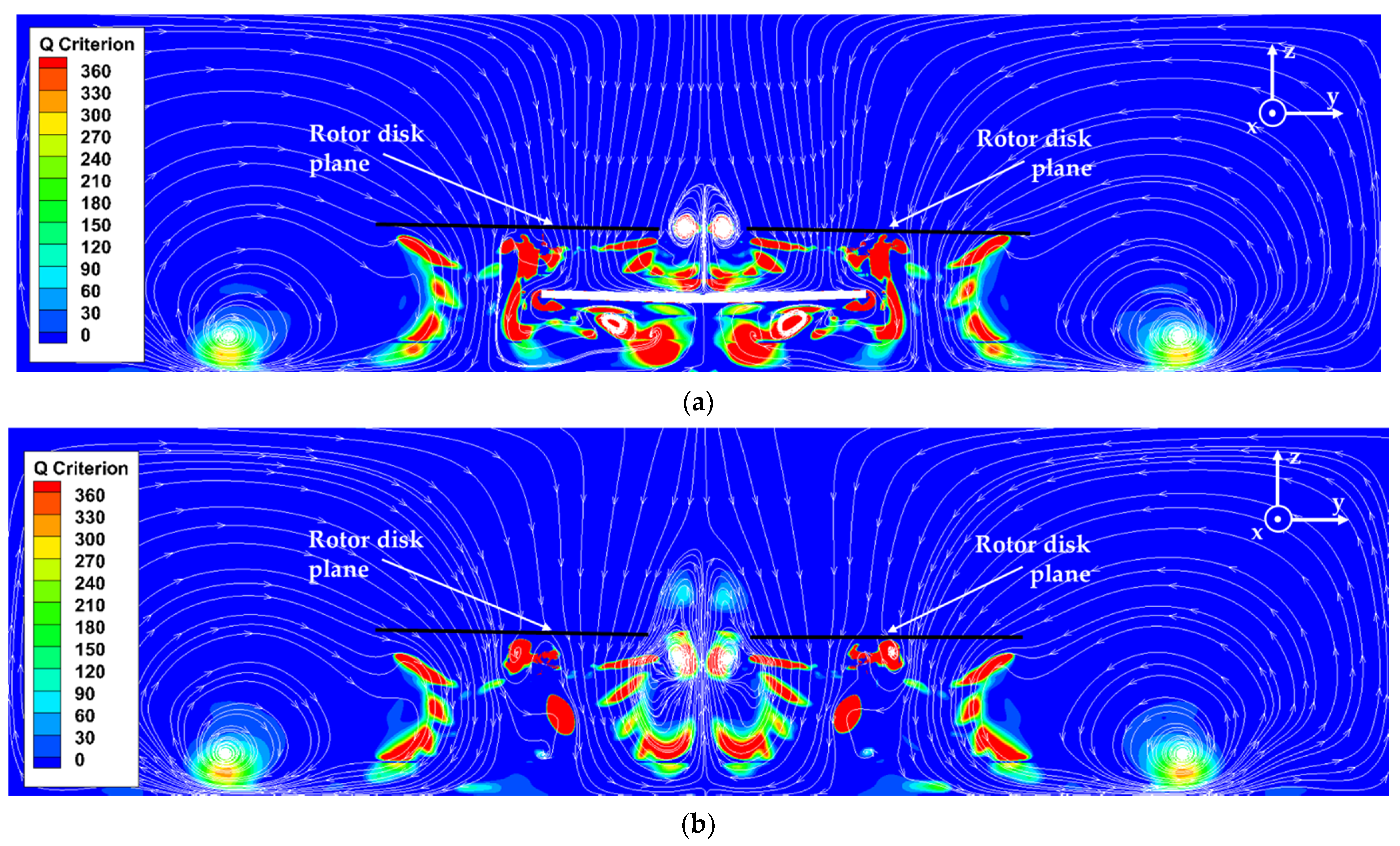
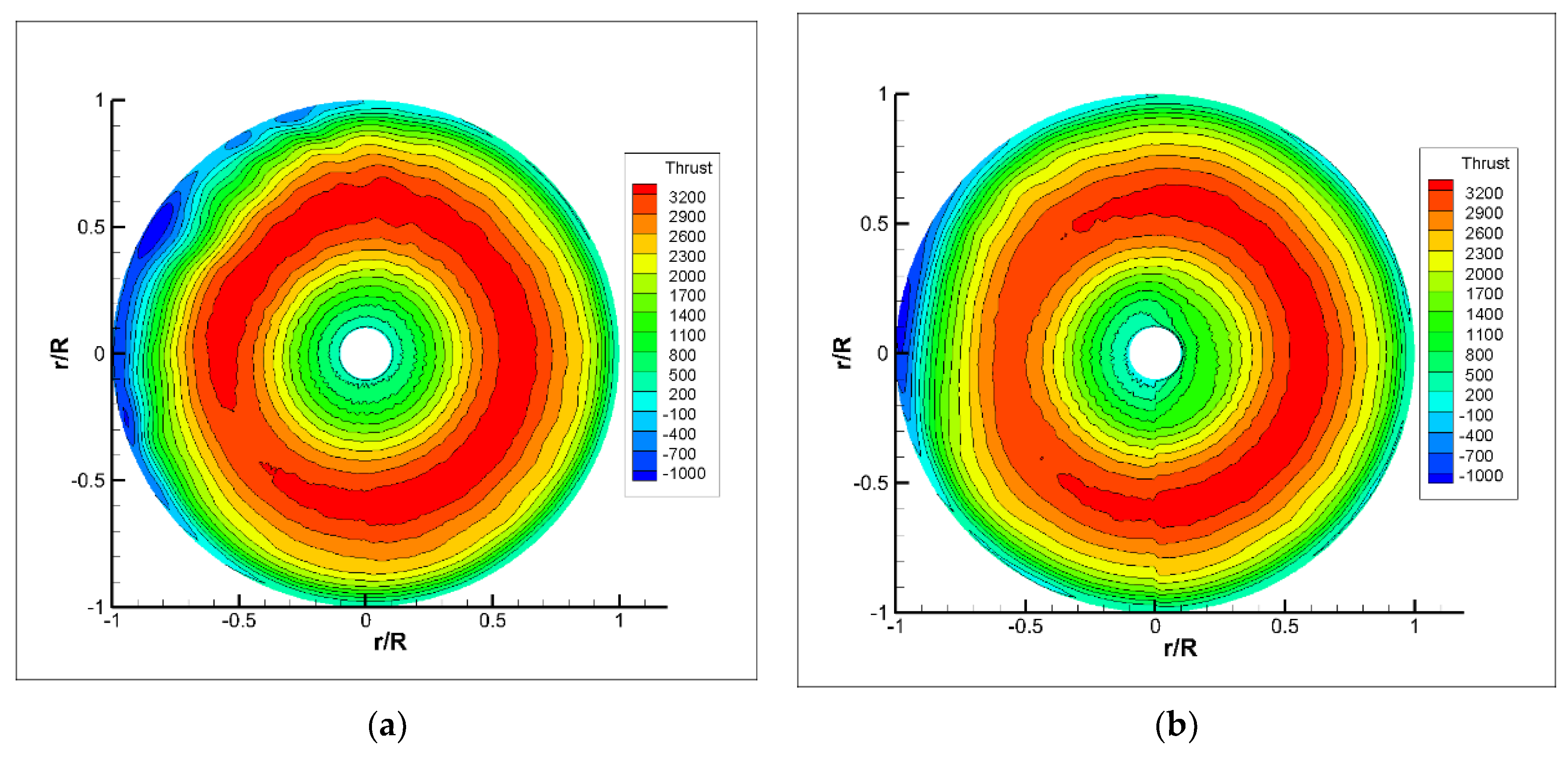
• When the ship was not moving, the fountain flow generated by the two rotors near the centerline of the fuselage caused a significant change in the spanwise thrust of the blade. The thrust weakened with the distance moving closer to the location of the fountain flow effect. The equivalent ground effect of the wing on the rotor was relatively weak, but the wing affected the fountain flow; thus, a low-thrust zone occurred on the retreating side.
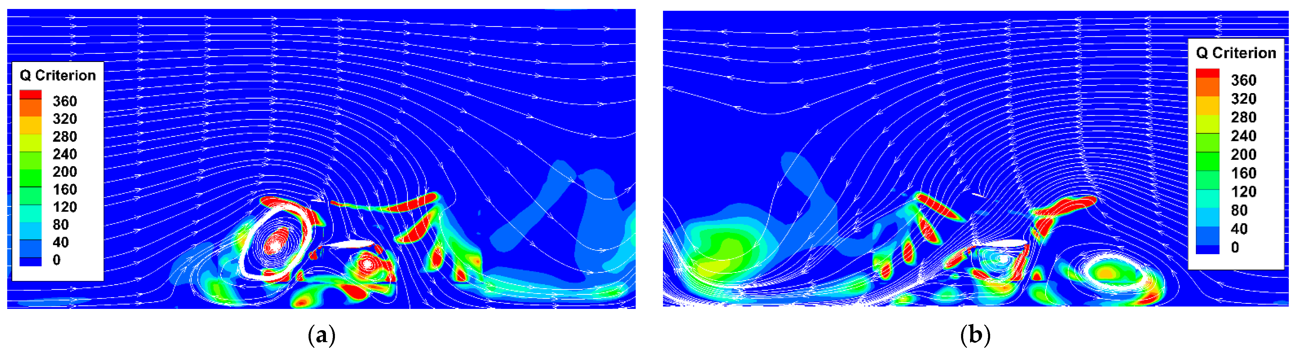
• When the ship was moving and the rotor was tilted backward, the wake rolled upward before it reached the ship’s deck, due to the interference of the wing vortex. The unstable flow caused large frequency fluctuations in the load at ψ = 360° because of the equivalent ground effect of the wing and the interference of the wing vortex.
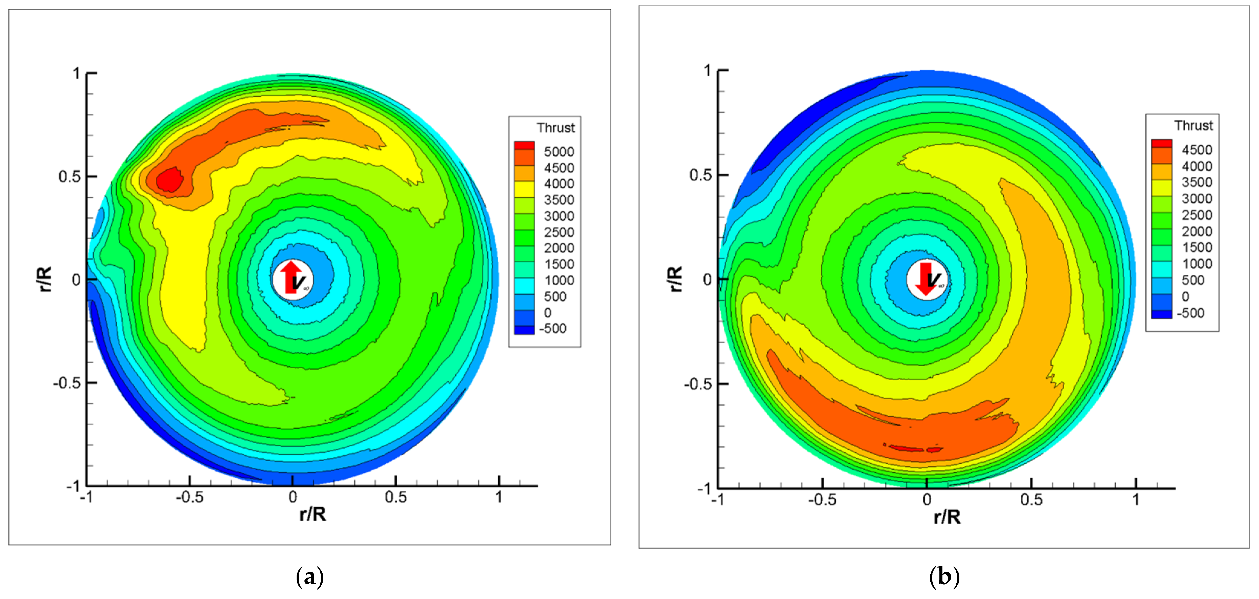
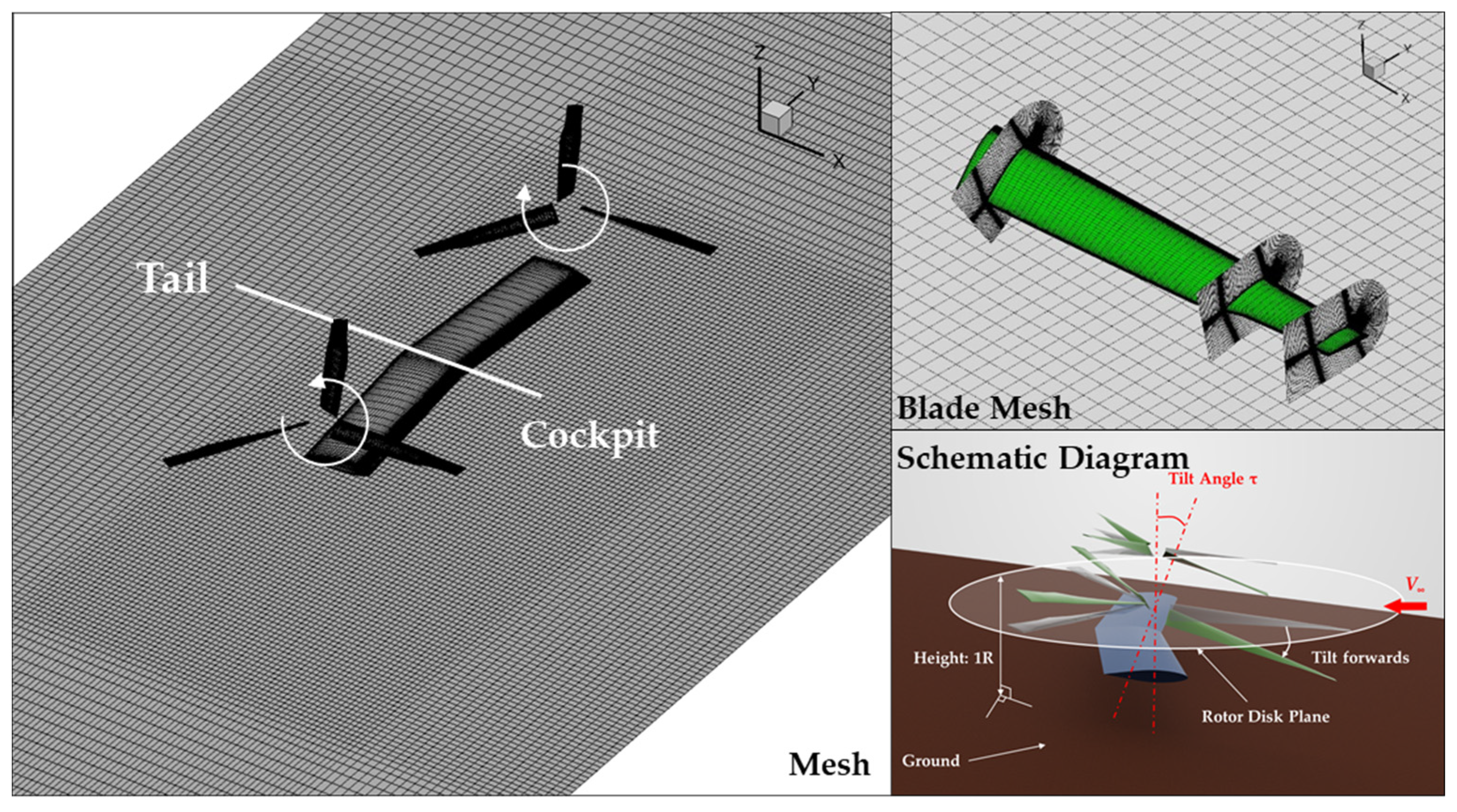
• When the tilt angle was zero, the chord line of the wing, the ship’s deck, and the rotor’s plane were almost parallel, and the equivalent ground effect of the wing on the rotor was less pronounced. In contrast, when the ship was moving and the rotor shaft was tilted, the three surfaces were not parallel. Thus, the equivalent ground effect of the wing increased the thrust of the rotor in the downstream direction of the sea wind. The wing significantly affected the rotor’s aerodynamic characteristics when the tiltrotor took off or landed with a small tilt angle.
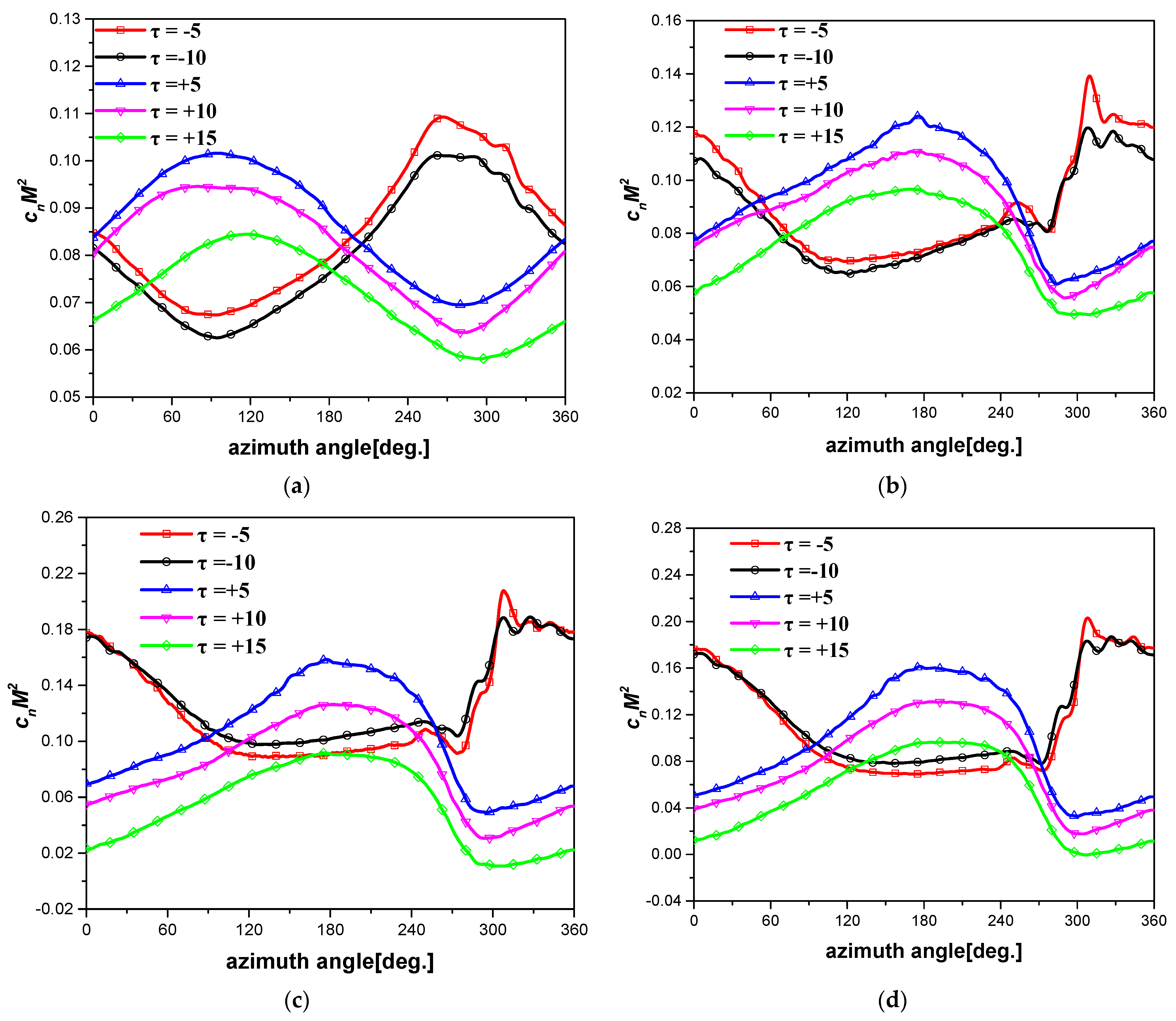
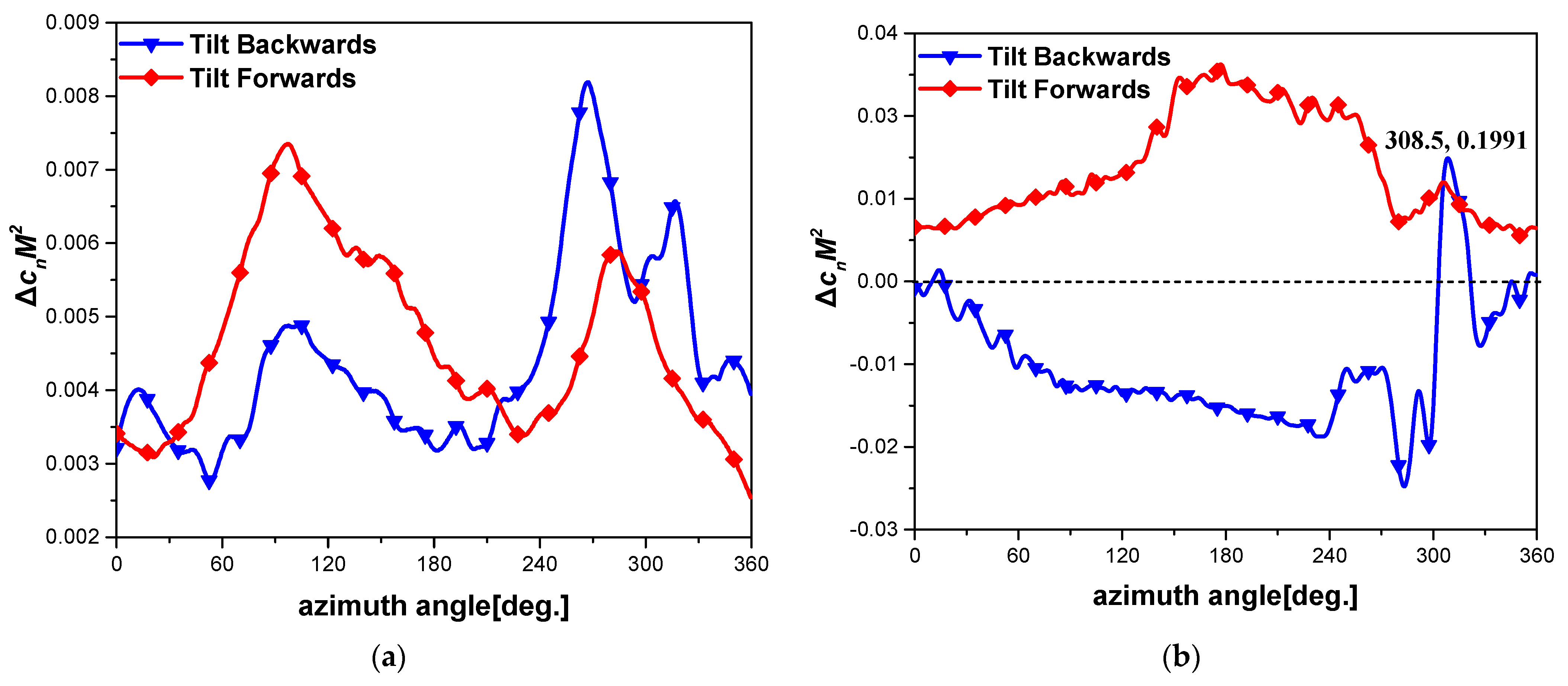
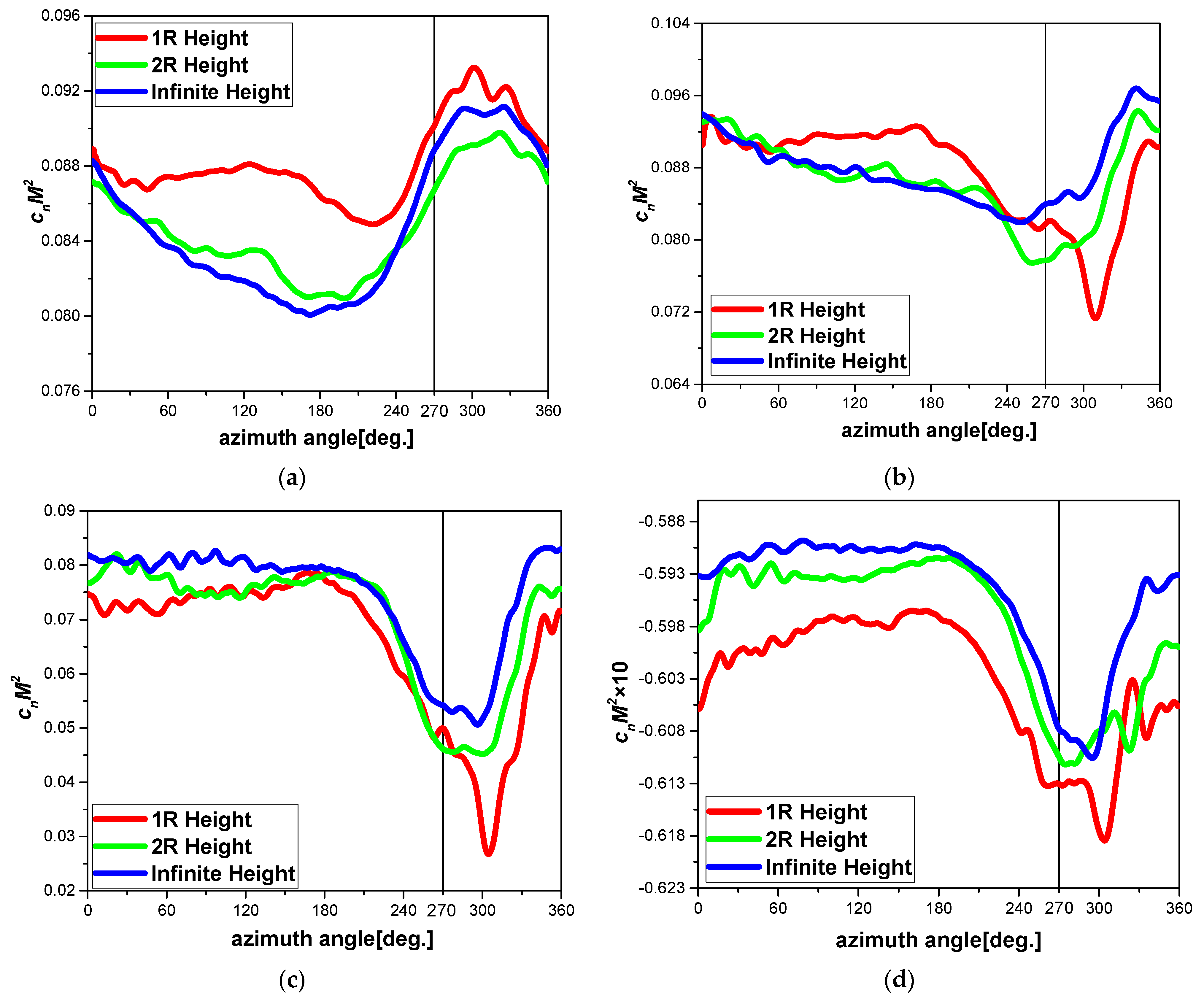
• During the take-off and landing of the tiltrotor with a small tilt angle, the normal forces of the 0.5R and 0.7R sections were higher for a smaller tilt angle than for a larger angle, regardless of whether the rotor was tilted forward or backward. In contrast, in the 0.8R section close to the blade tip, the normal force coefficients were not larger for a smaller tilt angle when the rotor was tilted backward except for the small range around ψ = 308°. In addition, the difference in the normal force coefficient between the 5° and 10° tilt angle sections was much smaller in section 0.8R than in section 0.5R.
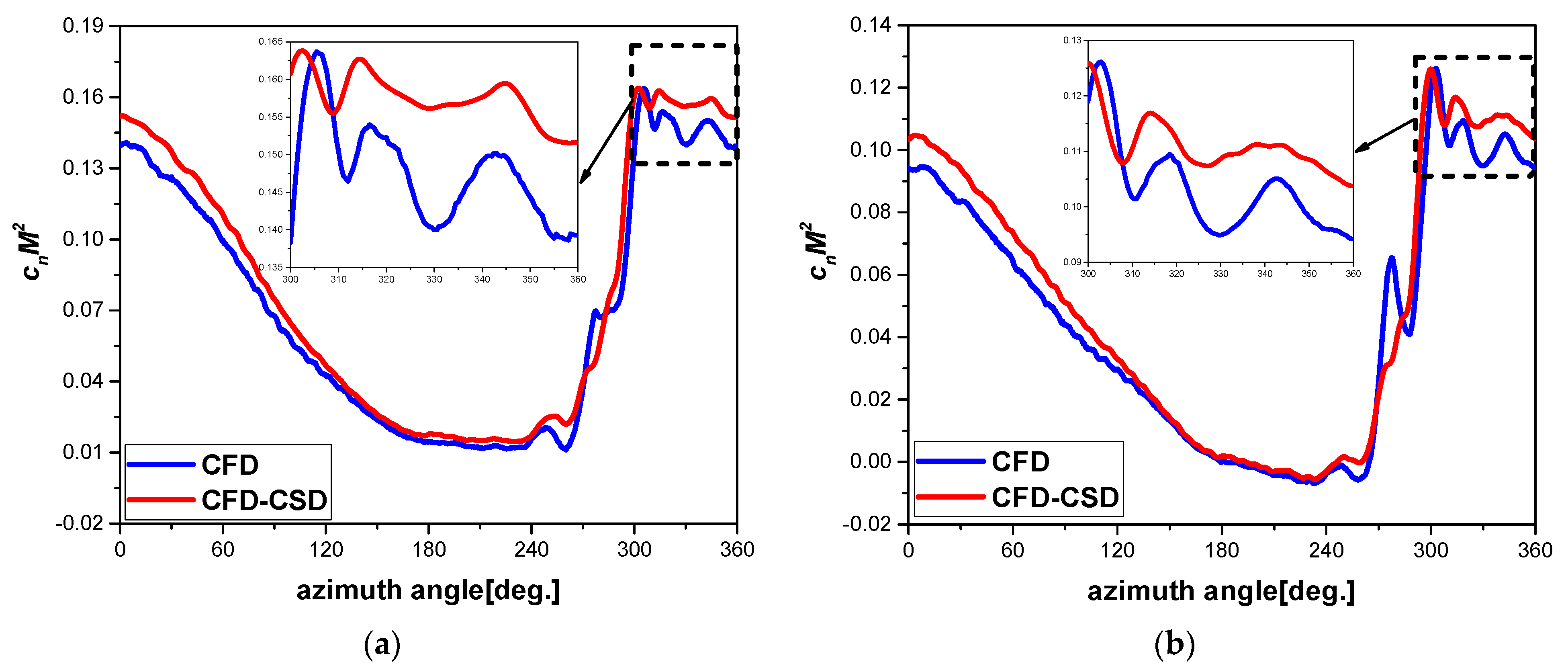
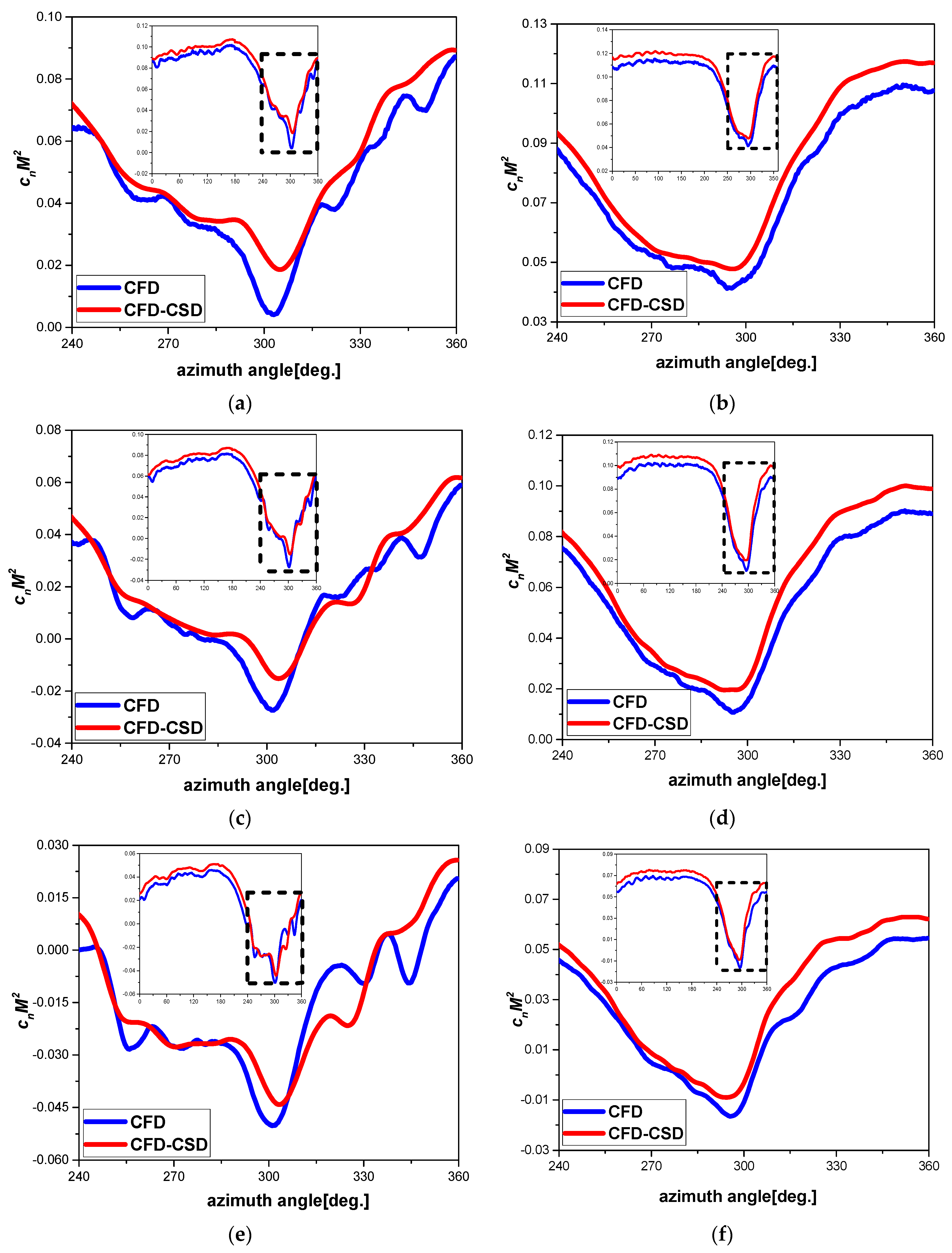
• The elastic deformation of the tiltrotor’s blade during shipboard take-off and landing decreases the fluctuations in the amplitude of the normal force at the rotor’s tip in one revolution. A comparison of the results obtained from the CFD and coupled CFD-CSD methods for a 5° backward tilt angle indicates that the elastic deformation reduces the amplitude of the thrust fluctuations caused by the interference of the wing vortex. The aerodynamic characteristics of the blade are more sensitive to elastic deformation in regions of higher aerodynamic force fluctuations.

In the future, a new CSD solver based on the finite element method will be implemented to obtain more precise deformation data, including blade warping and displacement.

References

1. Han, D.; Barakos, G.N. Transient Aeroelastic Response of a Rotor during Rotor Speed Transition in Forward Flight. J. Aircr. 2022, 1–7. [Google Scholar] [CrossRef]
2. Kucab, J.; Moulton, M.; Fan, M.; Steinhoff, J. The Prediction of Rotor Flows in Ground-Effect with a New Hybrid Method. In Proceedings of the 17th Applied Aerodynamics Conference, Norfolk, VA, USA, 28 June–1 July 1999; American Institute of Aeronautics and Astronautics: Norfolk, VA, USA, 1999. [Google Scholar]
3. Bhattacharyya, S.; Conlisk, A. The Structure of the Rotor Wake in Ground Effect. In Proceedings of the 41st Aerospace Sciences Meeting and Exhibit, Reno, NV, USA, 6–9 January 2003; American Institute of Aeronautics and Astronautics: Reno, NV, USA, 2003. [Google Scholar]
4. Kang, N.; Sun, M. Technical Note: Prediction of the Flow Field of a Rotor in Ground Effect. J. Am. Helicopter Soc. 1997, 42, 195–198. [Google Scholar] [CrossRef]
5. Hwang, J.Y.; Kwon, O.J. Assessment of S-76 Rotor Hover Performance in Ground Effect Using an Unstructured Mixed Mesh Method. Aerosp. Sci. Technol. 2019, 84, 223–236. [Google Scholar] [CrossRef]
6. Lakshminarayan, V.K.; Kalra, T.S.; Baeder, J.D. Detailed Computational Investigation of a Hovering Microscale Rotor in Ground Effect. AIAA J. 2013, 51, 893–909. [Google Scholar] [CrossRef]
7. Young, L.A. Simulated Tiltrotor Aircraft Operation in Close Proximity to a Building in Wind and Ground-Effect Conditions. In Proceedings of the 15th AIAA Aviation Technology, Integration, and Operations Conference, Dallas, TX, USA, 22–26 June 2015; American Institute of Aeronautics and Astronautics: Dallas, TX, USA, 2015. [Google Scholar]
8. Potsdam, M.A.; Strawn, R.C. CFD Simulations of Tiltrotor Configurations in Hover. J. Am. Helicopter Soc. 2005, 50, 82–94. [Google Scholar] [CrossRef] [Green Version]
9. Ye, L.; Zhang, Y.; Yang, S.; Zhu, X.; Dong, J. Numerical Simulation of Aerodynamic Interaction for a Tilt Rotor Aircraft in Helicopter Mode. Chin. J. Aeronaut. 2016, 29, 843–854. [Google Scholar] [CrossRef] [Green Version]
10. Xiao, Y.; Xu, G.-H.; Shi, Y.-J. Aeroelastic Analysis of Helicopter Rotors Using Computational Fluid Dynamics/Comprehensive Analysis Loose Coupling Model. Proc. Inst. Mech. Eng. Part G J. Aerosp. Eng. 2015, 229, 621–630. [Google Scholar] [CrossRef]
11. Hu, Z.; Xu, G.; Shi, Y. A Robust Overset Assembly Method for Multiple Overlapping Bodies. Int. J. Numer. Methods Fluids 2021, 93, 653–682. [Google Scholar] [CrossRef]
12. Hu, Z.; Xu, G.; Shi, Y. A New Study on the Gap Effect of an Airfoil with Active Flap Control Based on the Overset Grid Method. Int. J. Aeronaut. Space Sci. 2021, 22, 779–801. [Google Scholar] [CrossRef]
13. Sun, Y.; Xu, G.; Shi, Y. Numerical Investigation on Noise Reduction of Rotor Blade-Vortex Interaction Using Blade Surface Jet Blowing. Aerosp. Sci. Technol. 2021, 116, 106868. [Google Scholar] [CrossRef]
14. Ye, Z.; Zhan, F.; Xu, G. Numerical Research on the Unsteady Evolution Characteristics of Blade Tip Vortex for Helicopter Rotor in Forward Flight. Int. J. Aeronaut. Space Sci. 2020, 21, 865–878. [Google Scholar] [CrossRef]
15. Bauchau, O.; Ahmad, J. Advanced CFD and CSD Methods for Multidisciplinary Applications in Rotorcraft Problems. In Proceedings of the 6th Symposium on Multidisciplinary Analysis and Optimization, Bellevue, WA, USA, 4–6 September 1996; American Institute of Aeronautics and Astronautics: Bellevue, WA, USA, 1996. [Google Scholar]
16. Pomin, H.; Wagner, S. Aeroelastic Analysis of Helicopter Rotor Blades on Deformable Chimera Grids. J. Aircr. 2004, 41, 577–584. [Google Scholar] [CrossRef]
17. Romani, G.; Casalino, D. Rotorcraft Blade-Vortex Interaction Noise Prediction Using the Lattice-Boltzmann Method. Aerosp. Sci. Technol. 2019, 88, 147–157. [Google Scholar] [CrossRef]
18. Min, B.-Y.; Sankar, L.N.; Bauchau, O.A. A CFD–CSD Coupled-Analysis of HART-II Rotor Vibration Reduction Using Gurney Flaps. Aerosp. Sci. Technol. 2016, 48, 308–321. [Google Scholar] [CrossRef]
19. Lim, J.W. Consideration of Structural Constraints in Passive Rotor Blade Design for Improved Performance. Aeronaut. J. 2015, 119, 1513–1539. [Google Scholar] [CrossRef]
20. Khawar, J.; Ghafoor, A.; Chao, Y. Validation of CFD-CSD Coupling Interface Methodology Using Commercial Codes. Int. J. Numer. Methods Fluids 2011, 65, 475–495. [Google Scholar] [CrossRef]
21. Jung, Y.S.; Yu, D.O.; Kwon, O.J. Aeroelastic Analysis of High-Aspect-Ratio Wings Using a Coupled CFD-CSD Method. Trans. Jpn. Soc. Aeronaut. Space Sci. 2016, 59, 123–133. [Google Scholar] [CrossRef] [Green Version]
22. Goulos, I. Modelling the Aeroelastic Response and Flight Dynamics of a Hingeless Rotor Helicopter Including the Effects of Rotor-Fuselage Aerodynamic Interaction. Aeronaut. J. 2015, 119, 433–478. [Google Scholar] [CrossRef]
23. Wang, S.; Han, J.; Yun, H.; Chen, X. CFD-CSD Method for Coupled Rotor-Fuselage Vibration Analysis with Free Wake-Panel Coupled Model. Proc. Inst. Mech. Eng. Part G J. Aerosp. Eng. 2021, 235, 1343–1354. [Google Scholar] [CrossRef]
24. Löhner, R. Robust, Vectorized Search Algorithms for Interpolation on Unstructured Grids. J. Comput. Phys. 1995, 118, 380–387. [Google Scholar] [CrossRef]
25. Friedmann, P.P.; Glaz, B.; Palacios, R. A Moderate Deflection Composite Helicopter Rotor Blade Model with an Improved Cross-Sectional Analysis. Int. J. Solids Struct. 2009, 46, 2186–2200. [Google Scholar] [CrossRef] [Green Version]
26. Xing, Y.; Zhang, H.; Wang, Z. Highly Precise Time Integration Method for Linear Structural Dynamic Analysis. Int. J. Numer. Methods Eng. 2018, 116, 505–529. [Google Scholar] [CrossRef]
27. Tung, C.; Caradonna, F.X.; Johnson, W.R. The Prediction of Transonic Flows on an Advancing Rotor. J. Am. Helicopter Soc. 1986, 31, 4–9. [Google Scholar] [CrossRef]
28. Yeo, H.; Potsdam, M. Rotor Structural Loads Analysis Using Coupled Computational Fluid Dynamics/Computational Structural Dynamics. J. Aircr. 2016, 53, 87–105. [Google Scholar] [CrossRef] [Green Version]
29. Felker, F.F.; Young, L.A.; Signor, D.B. Performance and Loads Data from a Hover Test of a Full-Scale Advanced Technology XV-15 Rotor; NASA TM-86854; NASA: Washington, DC, USA, 1986; 359p. [Google Scholar]
30. Van der Wall, B.G.; Burley, C.L.; Yu, Y.; Richard, H.; Pengel, K.; Beaumier, P. The HART II Test—Measurement of Helicopter Rotor Wakes. Aerosp. Sci. Technol. 2004, 8, 273–284. [Google Scholar] [CrossRef]
31. Smith, M.J.; Lim, J.W. An Assessment of CFD/CSD Prediction State-of-the-Art Using the HART II International Workshop Data. In Proceedings of the 68th Annual Forum of the American Helicopter Society, Fort Worth, TX, USA, 1–3 May 2012. [Google Scholar]
32. Liu, Y.; Anusonti-Inthra, P.; Diskin, B. Development and Validation of a Multidisciplinary Tool for Accurate and Efficient Rotorcraft Noise Prediction (MUTE); NASA: Washington, DC, USA, 2011; 74p. [Google Scholar]
33. Servera, G.; Beaumier, P.; Costes, M. A Weak Coupling Method between the Dynamics Code HOST and the 3D Unsteady Euler Code WAVES. Aerosp. Sci. Technol. 2001, 5, 397–408. [Google Scholar] [CrossRef]
Figure 1. Pre-classification results of the original criterion and ROAT: (a) result of the Löhner criterion; (b) result of the ROAT.
Aerospace 09 00261 g001
Figure 2. Grid system to simulate the flow field of a tiltrotor during shipboard take-off and landing.
Aerospace 09 00261 g002
Figure 3. Degrees of freedom of the Timoshenko beam.
Aerospace 09 00261 g003
Figure 4. Flowchart of the CFD-CSD coupling.
Aerospace 09 00261 g004
Figure 5. Advanced technology blade of the XV-15 tiltrotor.
Aerospace 09 00261 g005
Figure 6. Normal force coefficient comparison of the four grid systems. (a) r/R = 0.85. (b) r/R = 0.9.
Aerospace 09 00261 g006
Figure 7. Frequency diagram of the Hart-II model rotor, predicted by the CSD model.
Aerospace 09 00261 g007
Figure 8. Sectional normal force at 87%R (mean removed and high-frequency content filtered): (a) original results; (b) error values of the results between the calculations in the present work and the experiment.
Aerospace 09 00261 g008
Figure 9. Iso-surface of the Q-criterion, colored according to velocity magnitude.
Aerospace 09 00261 g009
Figure 10. Pressure coefficient of the 7A blade with a high advance ratio (r/R = 0.975). (a) ψ = 150°. (b) ψ = 180°. (c) ψ = 210°.
Aerospace 09 00261 g010aAerospace 09 00261 g010b
Figure 11. Thrust distribution of the rotor at different heights: (a) 1R height, rotor with a wing; (b) 1R height, rotor without a wing.
Aerospace 09 00261 g011
Figure 12. Streamlines and contours of the Q criterion at 1R height (front view): (a) 1R height, rotors with a wing; (b) 1R height, rotors without a wing.
Aerospace 09 00261 g012
Figure 13. Normal force coefficient at different heights. (a) r/R = 0.5. (b) r/R = 0.7. (c) r/R = 0.8. (d) r/R = 0.95.
Aerospace 09 00261 g013
Figure 14. Comparison of the normal force in the last third of the period, obtained from the CFD and coupled CFD-CSD methods. (a) 1R Height r/R = 0.85. (b) Infinite height r/R = 0.85. (c) 1R Height r/R = 0.90. (d) Infinite height r/R = 0.90. (e) 1R Height r/R = 0.95. (f) Infinite height r/R = 0.95.
Aerospace 09 00261 g014
Figure 15. Side-view slices of the iso-surface of the Q-criterion at 0.5R: (a) τ = −5°; (b) τ = +5°.
Aerospace 09 00261 g015
Figure 16. Thrust distribution of the rotor in different states at 1R height: (a) τ = −5°; (b) τ = +5°.
Aerospace 09 00261 g016
Figure 17. Normal force coefficient versus azimuth angle. (a) r/R = 0.5. (b) r/R = 0.7. (c) r/R = 0.75. (d) r/R = 0.8.
Aerospace 09 00261 g017
Figure 18. Difference in the normal force coefficient from an absolute tilt angle of 5° to 10°. (a) r/R = 0.5. (b) r/R = 0.8.
Aerospace 09 00261 g018
Figure 19. Comparison of normal force coefficient for τ = −5° obtained from the CFD and coupled CFD-CSD methods. (a) r/R = 0.9. (b) r/R = 0.95.
Aerospace 09 00261 g019