SpaceDrones 2.0—Hardware-in-the-Loop Simulation and Validation for Orbital and Deep Space Computer Vision and Machine Learning Tasking Using Free-Flying Drone Platforms

Abstract

The proliferation of reusable space vehicles has fundamentally changed how assets are injected into the low earth orbit and beyond, increasing both the reliability and frequency of launches. Consequently, it has led to the rapid development and adoption of new technologies in the aerospace sector, including computer vision (CV), machine learning (ML)/artificial intelligence (AI), and distributed networking. All these technologies are necessary to enable truly autonomous “Human-out-of-the-loop” mission tasking for spaceborne applications as spacecrafts travel further into the solar system and our missions become more ambitious. This paper proposes a novel approach for space-based computer vision sensing and machine learning simulation and validation using synthetically trained models to generate the large amounts of space-based imagery needed to train computer vision models. We also introduce a method of image data augmentation known as domain randomization to enhance machine learning performance in the dynamic domain of spaceborne computer vision to tackle unique space-based challenges such as orientation and lighting variations. These synthetically trained computer vision models then apply that capability for hardware-in-the-loop testing and evaluation via free-flying robotic platforms, thus enabling sensor-based orbital vehicle control, onboard decision making, and mobile manipulation similar to air-bearing table methods. Given the current energy constraints of space vehicles using solar-based power plants, cameras provide an energy-efficient means of situational awareness when compared to active sensing instruments. When coupled with computationally efficient machine learning algorithms and methods, it can enable space systems proficient in classifying, tracking, capturing, and ultimately manipulating objects for orbital/planetary assembly and maintenance (tasks commonly referred to as In-Space Assembly and On-Orbit Servicing). Given the inherent dangers of manned spaceflight/extravehicular activities (EVAs) currently employed to perform spacecraft maintenance and the current limitation of long-duration human spaceflight outside the low earth orbit, space robotics armed with generalized sensing and control and machine learning architecture have a unique automation potential. However, the tools and methodologies required for hardware-in-the-loop simulation, testing, and validation at a large scale and at an affordable price point are in developmental stages. By leveraging a drone’s free-flight maneuvering capability, theater projection technology, synthetically generated orbital and celestial environments, and machine learning, this work strives to build a robust hardware-in-the-loop testing suite. While the focus of the specific computer vision models in this paper is narrowed down to solving visual sensing problems in orbit, this work can very well be extended to solve any problem set that requires a robust onboard computer vision, robotic manipulation, and free-flight capabilities.

1. Introduction

Over the past 65 years, humanity has had a constant presence in space, 21 of which have been a continuous human presence. The various orbital and deep space assets deployed during this time have, on occasion, required maintenance. The ability to successfully conduct space-based servicing has been a function of two constraints—cost and availability of maintenance assets. Thus, on-orbit servicing was confined to the most expensive space assets such as the International Space Station and Hubble Space Telescope. Over the last decade, the aerospace industry has reduced the launch cost, thus facilitating access to space significantly. This paper focuses on the latter of these constraints, which is space-based maintenance capability. Spaceborne maintenance tasking has traditionally been completed by astronauts performing Extravehicular Activities ((EVAs) more commonly known as spacewalks) outside the spacecraft or station to carry out maintenance, assembly, or upgrades of the existing infrastructure. Offloading these tasks to robotic platforms will be the next milestone for true deep space exploration, especially as new missions venture further away from the Earth. Deep space missions will also pose a constraint on the manned crews to operate or survive in a hostile environment for longer period. However, methods to test and validate autonomous space robotics systems is still a relatively new field of study. Figure 1 illustrates the transition from past methods of orbital maintenance to future robotic operations.

The aerospace industry has developed clever ways to simulate the physical and visual environments of space. Facilities such as the zero-gravity simulation of NASA’S Neutral Buoyancy Lab [2], Zero Gravity Facility [3], spacecraft vacuum testing carried out at NASA’s Thermal Vacuum Chambers [4], and several others summarized here [5] are world-class facilities. Most of these house capabilities are unique to that institution or are found only in a few other facilities around the world. The inability to easily recreate these facilities presents the first challenge to researchers aiming to tackle large fundamental scientific and engineering questions in the domain of space. Requesting lab time in these large high-demand multi-million dollar facilities is either impossible or prohibitively difficult to most organizations, including universities. Thus, several institutions have endeavored to recreate some of these capabilities at a smaller and cost-effective scale [6,7,8,9] with impressive results, all of which have been summarized in Figure 2.

These methods or facilities replicate dynamic or visual space domain parameters at scales large enough to answer the posed questions but small enough to be operated by teams of students with operating costs that are orders of magnitude less. This paper narrows down the following four problem sets related to optical sensing, domain randomization, and visual simulation for robotic manipulation to combine the capabilities of maneuver testing with onboard computer vision: (1) demonstrate the feasibility of simulated visual environments to supplement or completely replace real-world orbital or deep space imagery for the purposes of training neural networks to perform automated tasks; (2) evaluate the impact of domain randomized data sets on neural network performance for space applications; (3) deploy such a system onboard a free-flying drone platform performing onboard computer vision to provide real-time sensing for real-world robotic manipulation; (4) lastly, deploy the previously mentioned integrated system within a theater projection facility capable of projecting high fidelity environment to provide hardware-in-the-loop visual simulation and flight testing to further expand Validation and Verification (V&V) capabilities.

This project is divided into two major sections. The first section, detailed in Figure 3, focuses on the development, testing, and evaluation of the computer vision neural network architecture, synthetic imagery, and domain randomization methods when applied to space-based applications.

The second section, detailed in Figure 4, then employs the resulting neural network models onboard free-flying platform to perform localization and object capture within a projected simulation space, enabling hardware-in-the-loop testing. The authors are aware of the differences in dynamics between atmospheric propeller powered drone systems and floating orbital platforms. However, the current drone platform offers four uncoupled and unrestricted degrees of freedom for motion simulation, which is one more than a traditional air bearing table used in the past by organizations such as NASA for the SPHERES program [10] or IEEE’s Formation Control Testbed (FCT) [8]. Future work will incorporate full uncoupled 6DOF (six degree of freedom) motion via an omni-directional drone with via a relative-motion PID (Proportional–Integral–Derivative) controller, detailed in the future works section.

2. Motivation

One of the most common automated/semi-automated orbital tasks within the aerospace industry is position estimation for rendezvous and docking operations (RPOs) [11,12]. These docking procedures are most often performed with cooperative spacecraft methods. These methods are by far the safest and most effective means of docking two or more spacecrafts. However, given the current push to solve the growing space debris problem [13] and future missions to damaged or non-functional spacecraft/stations, uncooperative RPO is another key enabling technology. The uncooperative spacecraft problem set can also be extended to In-Space Assembly operations. It is unlikely that every material necessary for orbital construction, such as truss beams, panels, electrical harnesses, etc., will have their own dedicated onboard cooperative ranging equipment, especially if those components are built using the proposed methods of orbital- and planetary-based additive manufacturing. Thus, identifying, classifying, and tracking objects of interest will need to be conducted via onboard sensing of the manipulating spacecraft or robotic system in a delicate zero-G pick-and-place operation.

Several computer vision and deep learning architectures have been recently applied to space-based applications in an attempt to solve a number of tasks, including orbital determination [14], navigation [15,16], mission planning and optimization [17,18], and control [19,20]. However, past and current uncooperative autonomous and semi-autonomous RPOs rely on time-consuming and ungeneralized hand-engineered features or prior knowledge of the satellite/station orientation. We have demonstrated a highly generalized process by leveraging new, efficient Convolution Neural Networks (CNNs), such as YOLOv5 [21], coupled with domain randomization.

In order to apply machine learning and computer vision architectures, thousands of images are needed to adequately train a model capable of reliably classifying any given object of interest. Obtaining such data sets is usually easy to do for most Earth-based computer vision problems. Obtaining usable image data from all possible angles and orientations relative to any given camera frame within the space domain is either prohibitively expensive or impossible in most use cases. In the case of In-space Assembly, most, if not all, construction materials will only exist in a CAD model before fabrication on orbit. If such materials are manufactured on Earth, orbital optical imagery cannot be simulated on Earth without the use of special synthetically generated backgrounds and lighting.

Perhaps the most pressing real-world example of this problem would be that of the newly launched James Webb Telescope (JWST), synthetically rendered in Figure 5. Unlike its predecessor, the Hubble Telescope, the James Webb’s parking orbit at L2 is substantially further away than Hubble’s low earth orbit, thus making repair operations a far more challenging task. In order to service the JWST and other deep space assets like it, the autonomous and semi-autonomous capabilities described earlier will need to be solved. JWST has just enough fuel reserve to maintain its orbit for 20 years. This constraint establishes a real-world timeline to develop, test, and deploy these systems to save a 10 billion dollar asset and other deep space infrastructures.

3. Research Questions

The objective of this paper is to better understand how we can leverage synthetic world-building to train computer vision models and how augmentations to those data affect performance in an effort to develop and ultimately deploy autonomous robotic platforms for generalized assembly and maintenance tasks within the challenging dynamic environment inherent to the space domain. This paper aims to construct the necessary testbed needed to answer the questions posed below.

• Can synthetic data be used for reliable real-world object tracking?
• Can domain randomization and data augmentation be used to increase cross-domain computer vision performance?
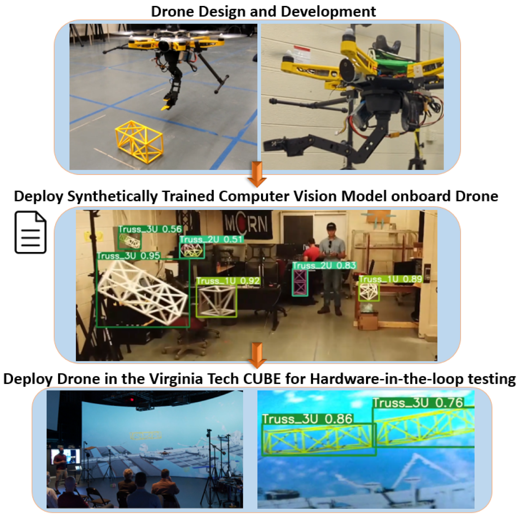
• Can synthetically trained computer vision models be used for Hardware-in-the-loop testing, sensing, and localization for real-world applications?

4. State of the Art

4.1. Domain Randomization

Domain randomization [22] is built upon the theory that with enough variability in a simulation, the real world will eventually appear to the model as just another variation. This would enable the model to perform in a wide range of optical perturbations when attempting to classify a given object. A simple and perhaps unintuitive concept dependent on training a neural network on a wide variety of variations for a given object such as lighting, color, texture patterns, position, and size, effectively minimizing the source vs. target domain problem when attempting to port trained neural network models from one domain to another is a process called “cross-domain”. The concept was pioneered to solve disparities between the real world and physics simulations for robotic control applications instead of relying on time-consuming traditional system identification methods. This concept has since been adopted for computer vision applications in an effort to close the reality gap between synthetic data and real-world object classification. Domain randomization is used to improve the mean average precision of object detection algorithms, such as YOLO [21], Faster RNN [23], and R-FCN [24], by evaluating combinations of synthetic training data that yield the highest average precision when validated against the real-world test images. This can be accomplished in two ways: (1) altering the source simulation environment using animation and rasterization tools/software generally used for game development to change parameters such as color, lighting, and object size, which produces a vast range of variation but it is time-consuming and requires detailed knowledge of a given software; (2) imagery from an environment, synthetic or real-world, can apply any number of filters to change desired parameters. However, applying domain randomization at the post-processing level limits the amount of control when changing environmental parameters. This method is defined as an auxiliary domain [22]. Creating an auxiliary domain is often easier to implement, but it often employs other machine learning architectures to intelligently change images’ properties such as color and lighting automatically, which is prone to some error. The number of parameters that can be changed in an already rendered image is limited compared to pre-rendered images. Domain randomization can be further expanded with the addition of “distractor objects”, which are defined as objects of more random shapes, sizes, and colors designed to generate random information for the feature map to extract, preventing the model from over-fitting.

4.2. Physical Simulation

Physical reality space simulation methods often require a physical object such as a robot that can be used in lieu of the celestial body that is being simulated. These simulations often go as far as using light fixtures and testbeds to recreate the lighting and degrees of freedom that can only be found in space.

For example, Johns Hopkins University leverages physical simulations to visually recreate night sky celestial bodies [25] using an all-black 4 ft diameter acrylic hemispherical dome via 100 light-emitting diodes (LEDs), thus enabling the simulation and testing of celestial navigation systems. Other organizations interested in physical free-floating 6DOF motion simulations tackle this problem by using robotic apparatuses combined with an air-bearing testbed. The formation control testbed developed by NASA was used to simulate the relative motion of a spacecraft. This testbed, at the time of its development, was comprised of three robots, each equipped with sensors, actuators, and processors to mimic multi-spacecraft formation flying without the need to be in microgravity [8].

4.3. Synthetic/Virtual Reality Space Simulation

Synthetic visual simulation can be just as advantageous as a physical simulation, as previously mentioned. Organizations such as the United States Naval Academy have conducted studies aimed at performing spacecraft attitude initialization by using Blender (a game engine and rasterization software) to render a Dragon X model at varying angles relative to a global light source to emulate the sun [7]. After systematically labeling the resultant images defined by Euler angle rotations at intervals of 10 degrees relative to the camera frame and using the AlexNet [26] CNN Framework, this methodology yielded a spacecraft angle accuracy of 95%.

Similarly, Airbus’s SurRender [27] image-rendering software is specifically designed to provide detailed realistic lighting for celestial surface imagery (e.g., Mars, asteroids, and orbital debris) to test and improve vision-based navigation (VBN) algorithms. It addresses some of the most problematic synthetic imagery challenges such as realistic light propagation, secondary illumination, and subpixel limb by using ray tracing, a new lighting technology recently made practical by newer and faster computing hardware. Having gone through a formal qualification process with the European Space Agency (ESA), the SuRender Software is perhaps the most robust purpose-built API aimed at countering the lack of validation solutions for spaceborne systems. Our method to recreate a derivative of these environments are detailed in the following section.

5. Materials and Methods

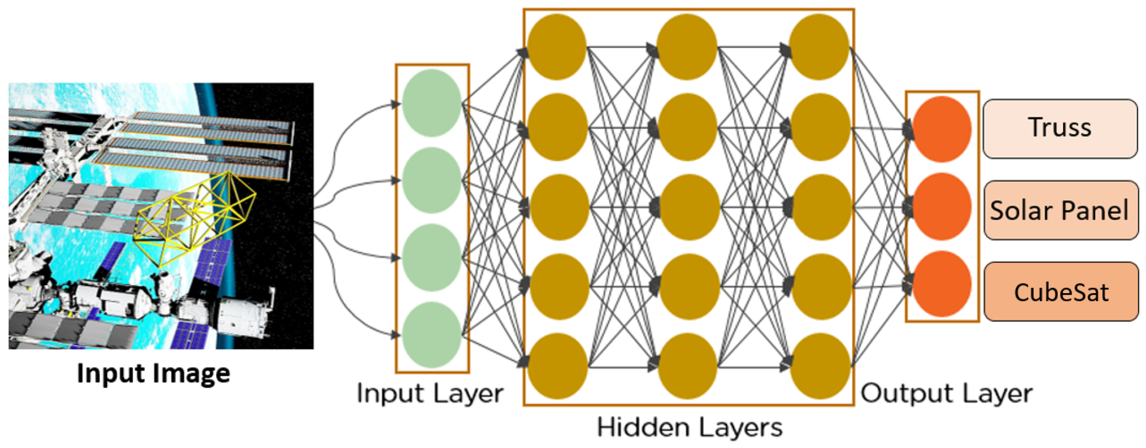
5.1. CNN Architecture Selection

Given the extremely rapid pace of machine learning algorithms, techniques, and methodologies, we will focus on those most relevant for this application. A dizzying array of convolution network architectures (CNNs) such as Faster R-CNN [28], RetinaNet [29], and Cross Stage Partial ResNet (CSPR) [30], each altering various parameters such as the size and number of neural network layers, nonlinear activation functions, pooling functions, image input, and many more are in constant evolution to increase a model’s performance. Additionally, the entire architecture can be changed, spawning subset architectures such as generative adversarial networks (GANSs) [31], DropConnect networks [32], and Deconvolutional networks [33]. The advantages and disadvantages of each can be narrowed down based on the power, time, or performance constraints for a given problem set.

We ultimately selected the “You Only Look Once” (YOLO) [34] architecture and a modified Pytorch framework (commonly known as YOLOv5). Today, the YOLO CNN architecture is widely accepted as one of the premier image classification algorithms due to its single-sweep approach of localizing and classifying objects. Whereas many modern models require several GPUs and batch sizes for training, the YOLO architecture can be trained and deployed on a single GPU, enabling us to deploy onboard edge compute devices comparable to those found on a small satellite payload.

Figure 6 illustrates a simplified example of using synthetic imagery as input to a given neural network for training in order to classify objects of interest, in this case, trusses, solar panels, and spacecraft.

5.2. Synthetic Reality Creation and Collection

Environmental factors can significantly influence the training of CNNs for the classification of images. It was therefore also imperative that the visual environmental conditions were captured as much as possible when using synthetic data. To generate a robust detection model that is capable of recognizing the relatively complex construction problem set consisting of several geometrically similar objects such as truss sections in a complex orbital regime, synthetic images were generated and stored. This was accomplished using a hyper-realistic Earth/Moon System environment with ray tracing where dynamic lighting was created at a resolution of 15,360 by 8640 pixels (16 K), as detailed in Figure 7. Factors such as asset distancing, perspective projection, dynamic lighting, model detail, color accuracy, etc., were considered to ensure that the synthetic data was representative of the desired environment.

The world-building process will differ between particular environments, but the overall development process is generally the same. Starting with a central landscape asset such as planet Earth or textured Mars landscape to serve as a foundation for the environment and world central point. Second, the lighting assets were created and placed in order to see real-time lighting effects on other assets as they are placed into the synthetic environment. Additional lighting parameters such as ray tracing or orbital glare effects are also generated in this step. Once lighting is established, any desired effects such as Earth albedo, cloud distortion, and sky box assets are added. Assets such as sun and moon models, star formations, or martian rock formations are either created or loaded from open source repositories to complete the overall environment. After all environmental assets are generated appropriately, objects of interest to the computer vision algorithm such as truss sections, solar panels, and ISS models are loaded to complete the synthetic scene. This completes the synthetic visual environment setup. The next step is to create the dynamic conditions governing how objects move and interact with each other in the synthetic world. These parameters include creating object motion via predefined animation sequences or dependent upon other object or world states such as object relative location or collision detection. Many of these parameters are controlled and modified via the unreal engine blue printing system. Finally, after the world has been created, object motion defined, and interaction parameters set, imagery is collected either through purpose built visual camera sequences designed to create pre-rendered scenes or, in the case of the domain randomization data sets, through direct game play interaction were a player is physically manipulating assets in the game world.

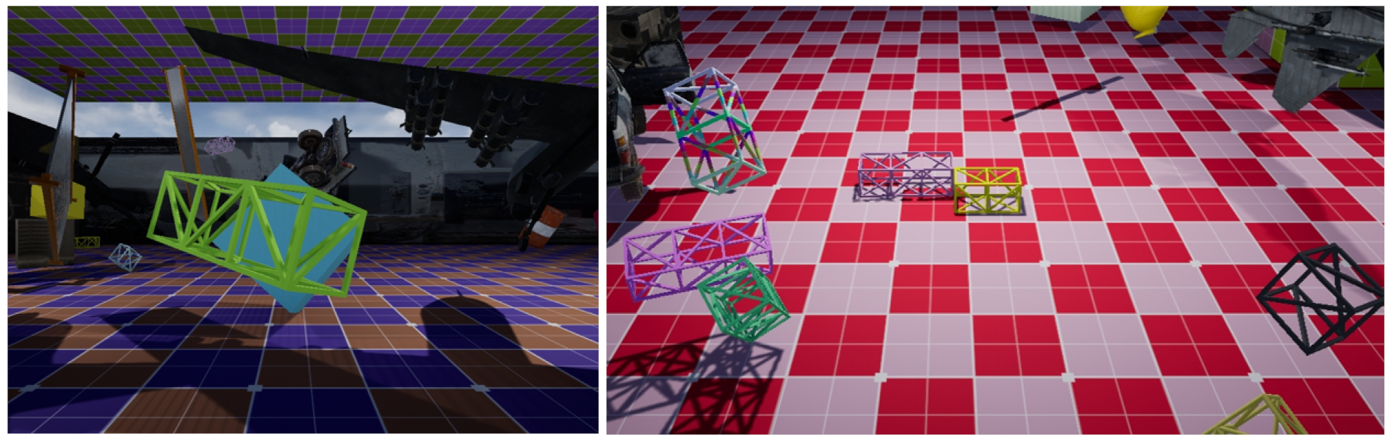
5.3. Synthetic Domain Randomization

To test the effects of domain randomization on a neural network’s ability to classify an object of interest, in this case, 3D printed truss sections for construction tasking, a highly randomized zero-gravity environment was developed within the Unreal Engine. All elements including the skybox, distractors, and objects of interest were programmed to randomize color and lighting effects over a given time frame or the same defined world state is met (illustrated in Figure 8). This method allowed us to generate thousands of highly randomized images across several object angles relatively quickly and allows us to perform domain randomization at the preprocessing level. Performing randomization operations before image rendering obviously allows for greater control, as opposed to applying filter effects on an image at the post-processing level, otherwise known as the “photo-shop” method. All Unreal Engine levels mentioned above can be found at [35] for open source use. Domain randomized synthetic environments are illustrated in Figure 8 and via video link (https://www.youtube.com/watch?v=bVemye0JU10&feature=youtu.be, accessed on 20 April 2022).

Once all assets in the environment have been rendered and motion modeled, a built-in camera tool captured the scene at 1080p. These media were then saved to a local hard drive and then labeled. Once all images were labeled, they were then organized and uploaded to a SQL Database for ease of use when training a CNN.

5.4. Porting CAD Models and Hardware into Synthetic Environments

To introduce CAD Models into the synthetic environment, 3D-printed STL files were injected into the Unreal Engine upon converting them to OBX files. To accomplish this, Blender was employed to convert the appropriate file types and adjust environment scaling. For example, most CAD files define the origin at (0,0) and build the object in quadrant one, thus keeping all values positive and effectively placing the origin in the corner. Attempting to accurately model dynamics creates a conflict due to UE4 (Unreal Engine 4) colocating an object’s center of gravity with the origin point, resulting in off-center dynamics when introducing object motion. To solve this, Blender is used to move object origin points to the geometric center of objects and set units of measurement to meters before porting. This workflow file conversion workflow is detailed in Figure 9.

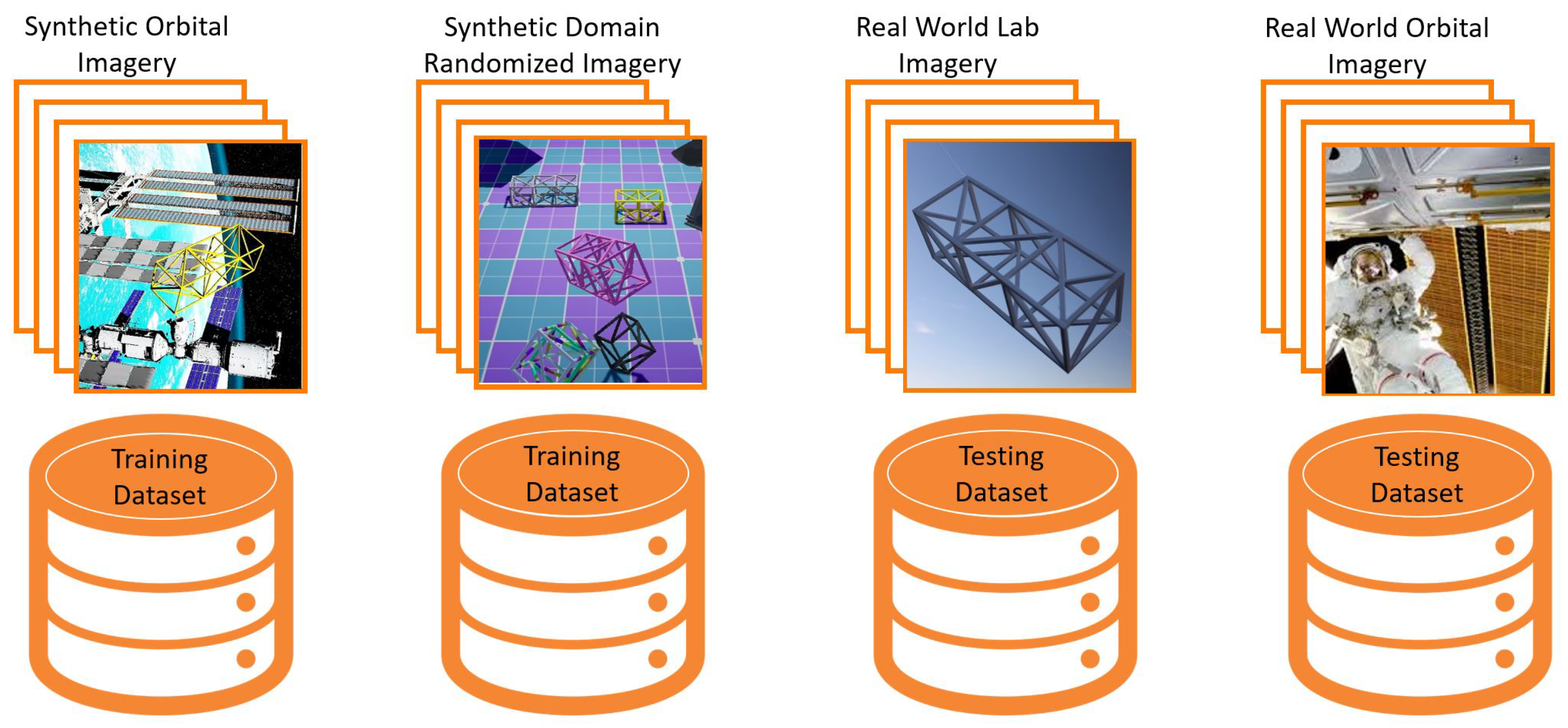
5.5. Division of Data Sets

Once labeled, all images were compiled and organized through experiments. Synthetic training images, real-world images, and synthetic testing images totaling over 15,000 unique images were separated into four primary data sets, as illustrated in Figure 10. Synthetic data sets serve as training data for the neural network, while real-world data sets are evaluated against synthetically trained CNN models to determine the feasibility of artificially trained neural networks for real-world inferencing applications. To further increase the amount of training data, some synthetic images were duplicated and a rotational transformation (90 degrees < $\theta$ < 180 degrees) was applied. This augmentation is acceptable and even necessary for orbital applications due to the free flying orbital rotation dynamics in space, while the “bottom” of an image is not always considered to be the “ground” as it is in typical terrestrial imagery. All data sets were then compiled to a database where they could be queried as needed by the CNN to run applicable experiments and evaluations.

5.6. Evaluation Metric

Average precision (AP) is one of the industry standards for the evaluation of a single class label in object classification and localization. Mean Average Precision (mAP) is the standard for the evaluation of an entire network of n class labels. Both of these metrics are functions of precision and recall (accuracy metrics that consider misclassification and classification accuracy rates. Precision and recall are defined below in Equations (1) and (2), respectively, where $TP=$ True Positive, $TN=$ True Negative, $FP=$ False Positive, and $FN=$ False Negative. The F1 score in Equation (3) combines both precision and recall via harmonic mean, later used in the results section.

$$\mathrm{Precision}=\frac{TP}{TP+FP}$$

(1)

$$\mathrm{Recall}=\frac{TP}{TP+FN}$$

(2)

$$F1=2·\frac{\mathrm{Precision}·\mathrm{Recall}}{\mathrm{Precision}+\mathrm{Recall}}$$

(3)

Average Precision is a measure of the area under the Precision–Recall Curve (PR Curve) [or p(r)] and is often defined as in Equation (4). The Mean Average Precision is simply defined in Equation (5).

$$AP={\int }_0^{1}p\left(r\right)dr$$

(4)

$$\mathrm{mAP}=\frac{1}{N}\sum _{i=1}^N{\mathrm{AP}}_i$$

(5)

Note that the subscripts on Mean Average Precision scores (often 50 or 75) generally denote the IoU threshold at which the score was taken. mAP(0.5) donates a 50% IoU, while mAP(0.5:0.95) donates IoU thresholds, from 50% to 95%.

6. Flight Hardware

Flight computer hardware and communication protocol are built using the companion computer infrastructure utilizing a commercial PID flight controller paired with a high-performance edge computer capable of executing complex workloads, including path planning, machine learning, and sensor integration. The first iteration of the SpaceDrones architecture [36] leveraged an onboard computer selected due to its lightweight and low-cost. At only 5 volts, the power requirements could be satisfied via GPO pins, simplifying the drone’s power distribution system while preserving limited power resources provided by an onboard battery. The hardware solution is cost-effective, costing under USD 100, and sufficient for many drone use cases. However, the demanding computational requirements of most neural networking applications are beyond the capabilities of nearly all such single board computers. In the past, drone sensor data such as imagery and point clouds could be sent “off drone” and interpolated using higher-end compute hardware not subject to the weight and power constraints of drone hardware. Instructions interpolated by a neural network architecture derived from drone sensor data could then be beamed back to the drone for execution. This off-drone compute capability is useful for a wide range of use cases but unrealistic for truly autonomous applications such as deep space exploration and tasking and situations requiring fast reaction times.

The recent introduction of a new line of Nvidia single-board edge computers capable of neural network tasking meets mass constraints for flight as a companion computer within the SpaceDrones architecture with a supplementary power distribution system capable of providing the required 19 volts of power required, as outlined in Figure 11.

7. SpaceDrones 2.0 Architecture

The SpaceDrones architecture is primarily built on top of the Robotic Operating System (ROS) [37]. The ROS framework allows the controllers to send and receive sensor data, neural network solutions, position data, and drone diagnostic data over a local area network via the publishing/subscribe functions. This local and/or distributed networking solution allows monitoring the neural network performance running onboard in real-time and associated drone performance instead of relying on locally stored data. Drone position data and any other object equipped with a tracker are interpolated by the Steam VR system and then sent to the drone or any other ROS node via the local network. These position data are then used by the onboard flight hardware to command or test vehicle motion. The full system architecture is shown in [38], consisting of a ground station used for command operations and downloading experimental data and the drone companion computer system.

The SpaceDrones API is capable of integrating two-position tracking systems (Opti-Track and Steam VR) for drone control, testing, and safety. Both systems utilize the MAVROS Package library for companion computer control over an onboard PID flight controller.

7.1. Lighthouse Tracking

The LIDAR lighthouse tracking suite is the solution utilized for this paper. Initially designed for VR asset tracking, it is an “inside-out” tracking solution that uses a proprietary tracking sensor with onboard IMU and photodiode tracking bay stations. This method is more limited in its ability to track nonrigid objects when compared to “outside-in” solutions, e.g., motion capture cameras such as Opti-Track. However, due to the rigid materials required to support drone flight, this constraint is not a factor. This system has the added benefit of being far cheaper to acquire and operate than turn-key camera positioning systems, and it easier to deploy in the field due to fewer hardware requirements and the tendency for sunlight in other IR-based camera tracking in outdoor environments. The lighthouse tracking system consists of at least one base station and one tracker, expandable to up to 16 base stations. The anchored base stations sweeps the room with laser pulses, while the trackers can detect and decode the laser pulses to solve their position and orientation relative to the base stations utilizing a model-based pose estimation method. Each base station has a motor that reflects, disperse, and rotates a thin laser fan at a fixed rate of 60 Hz. The laser signal was modulated so data can be transmitted from the base stations to the trackers. The system proved capable of resolving the position and orientation of the UAV at a rate of 120 Hz to sub-millimeter accuracy (as Figure 12 shows).

7.2. Target Localization

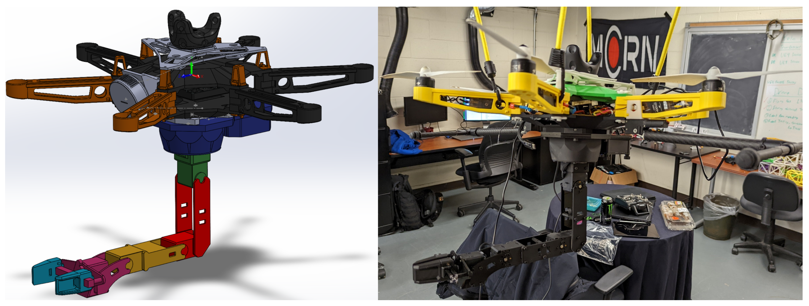
While YOLO can detect and output the 2D target position in the screen frame, any robotic operations involving object manipulation will require a localized 3D position of the target relative to either the camera body frame or local inertial frame. Here, we used an additional all-in-one sensor that included an RGB camera, a solid-state LiDAR module, and an onboard Inertial Measurement Unit (IMU). The RGB image stream can be fed directly to the YOLO detection algorithm for object detection, while the depth image stream can provide point cloud data for object localization shown in Figure 13.

The default Python script originally used to run the YOLO v5 neural network (detect.py) flying onboard the drone was modified to publish string message streams to the ROS network. The message stream contains basic detection results from each frame, which includes the name of the object, the confidence, and the relative 3D location of the object from the perspective of the camera. The LiDAR camera API has a built-in re-projection function that takes the 2D location of the object in the image provided by the YOLO detection program, as well as the distance from the camera to the specific depth pixels corresponding to the object location, and outputs the 3D location of the target voxel (volumetric pixel) from the point cloud.

The string message can then be interpreted further based on the location of the camera relative to the local inertial frame and completes the target localization process for each object detected. Software dependencies and data interlinks for neural network inferring, object localization, and capture are described in Figure 14.

Other than being geometrically similar and being difficult to distinguish, truss sections presented another problem. Given the porous structure of truss segments, a LiDAR scan can pass through the center point of a given voxel returned from a bounding box position, resulting in a depth measurement that is past the object we are trying to capture. To solve this problem, an internal box consisting of 70% of the original bounding box is scanned with a LiDAR sensor. To reduce computational time, every other pixel is skipped. The LiDAR return that is located closest to the center point of the original bounding box limits is taken as the depth measurement, which is then used for capture operations. The sensor integration order of operations is illustrated in Figure 15.

8. Drone Design

8.1. Drone Body

The SpaceDrones physical chassis has gone through many iterations of quad and hex copters, including off-the-shelf (OTS) solutions; however, no OTS bodies provided the internal volume needed to accommodate both the COTS controller and the new onboard computer. This shortfall necessitated the development of the in-house solution illustrated in Figure 16. The mass requirement for larger computers, two onboard sensors (camera/LiDAR and VR tracker), as well as an under-slung robotic arm, required a six rotor body to provide sufficient payload capacity.

8.2. Drone Power Distribution

The increased power consumption of the new onboard computer coupled with the need to power six motors, the radio controller, and camera systems simultaneously pulled more voltage than most off-the-shelf batteries could provide. Thus, two batteries connected in series delivered a combined 18 volts to the drone for flight operations. Additionally, a third independent 12-volt battery was added to power the under-slung robotic arm.

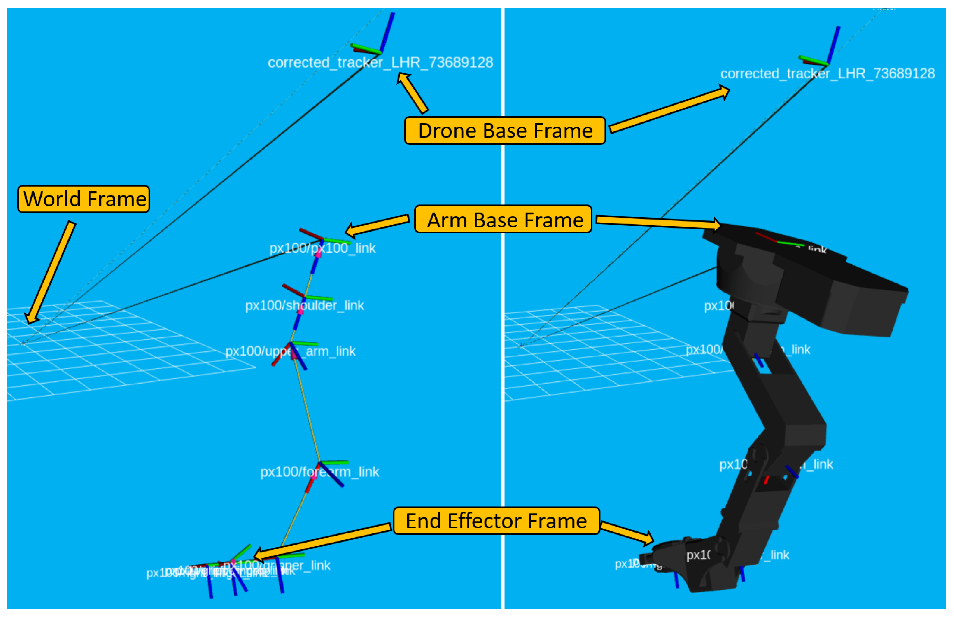
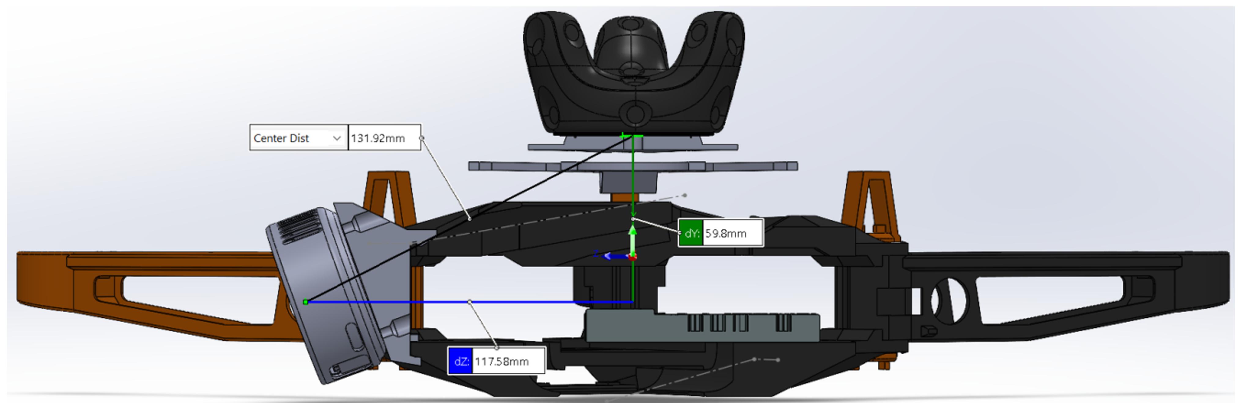
8.3. Drone Reference Frames

8.3.1. Drone Body Frames

The overall world reference frame is defined by the VR tracking system, and subsequent “world zero” can be defined to be anywhere by the user. Drone zero is defined by the VR Tracker located on the top of the drone. All drone transforms are derived from this zero. To locate objects in space relative to the drone frame, a known camera offset of 59.8 mm in the Y direction, 117.58 mm in the Z direction, as well as a 20-degree rotation along the X-axis defines the camera frame relative to the drone frame, as illustrated in Figure 17.

The camera being used onboard the drone is an Intel RealSense L515 sensor, so all rotations and translations relative to the camera will be referred to with “C” subscript. All rotations and translations relative to the steam VR Tracker located atop the drone will be denoted with the “T” subscript. The object of interest being localized is denoted as the “Target”. All rotations are defined in Figure 18, Figure 19 and Figure 20, where

$$\mathrm{subscript}\mathrm{T}=\mathrm{Tracker}\mathrm{Frame},\mathrm{subscript}\mathrm{C}=\mathrm{Camera}\mathrm{Frame},\mathrm{Target}=\mathrm{Target}\mathrm{Frame}$$

$$R=roll, P=pitch, Y=yaw$$

$$S=Sine, C=Cosine$$

Figure 18 illustrates the frame transformation to obtain the position of the L515 camera in the world inertial frame (Bottom), and the rotation matrix used from the steam tracker body frame to the inertial world frame (top).

Figure 19 illustrates the rotation of the L515 camera with respect to the world inertial frame.

Finally, Figure 20 illustrates the inertial frame of the object of interest or target detected by the drone-mounted camera using the computer relative to the world frame (bottom), via the rotation matrix from the camera to the inertial world frame (top). Effectively enabling object tracking in 3D space.

8.3.2. Robotic Arm Frames

The robotic arm mounted under the drone illustrated in Figure 21 is a 4DOF (four degree of freedom) PincherX 100 model powered by four Dynamixel smart servos. This robotic arm has a reach of 300 mm and a total rotating span of 600 mm, giving the robotic arm a total workspace that covers 112 percent of the drone’s 533.4 mm wingspan. Drone motion and the end effector position is governed by imagery and LiDAR sensor input data that have been interpolated by the onboard neural network detailed in the Target Localization section. Once an object of interest has been identified, its 3D location is used to drive the applicable inverse kinematics (IK) required to execute a successful object capture.

8.3.3. Robotic Arm Airborne Inverse Kinematics

The robotic arm’s base frame is maneuvered into place for object capture by the drone. The base frame of the arm is governed by the motion of the drone base frame, which in turn is governed by the overall world frame tracked by the VR world space diagrammed in Figure 22. Once an object is identified via computer vision, the drone controller maneuvers to the object, placing the arm within reach of the robot arm’s workspace, any error between the drone’s position and the object’s position will be corrected within the reach of the robotic arm. Once in position, an inverse kinematic (IK) controller calculates the distance between the object and the current end-effector position, then maneuvers the end effector to execute capture.

The robotic arm is equipped with three revolute motor joints that drive the end effector position and additional motor controlling gripper open and close functions. Desired robotic arm motion is calculated using the Jacobian iterative inverse kinematics method defined in Equations (6) through (10).

$p_i=$ the vector from the origin of the world coordinate system to the origin of the i-th link coordinate system;

$p=$ the vector from the origin to the end effector end; $z=$ the i-th joint axis;

$J=$ Jacobian Matrix;

$\Delta p=$ End Effector Position;

$\theta ={\theta }_1,{\theta }_2,\cdots ,{\theta }_n$.

$$\begin{array}{cc}\hfill & J\left(\theta \right)=\left(\begin{array}{ccc}{j}_{P1}\hfill & \hfill & j_{P_n}\hfill \\ \hfill & \dots \hfill & \\ j_{o1}\hfill & \hfill & j_{o_n}\hfill \end{array}\right)\hfill \end{array}$$

(6)

$$\begin{array}{cc}\hfill & \left[\begin{array}{c}{j}_{Pi}\hfill \\ j_{oi}\hfill \end{array}\right]=\left\{\begin{array}{c}\left[\begin{array}{c}{z}_{i-1}\\ 0\end{array}\right]\mathrm{for}\mathrm{a}\mathrm{prismatic}\mathrm{joint}\\ \left[\begin{array}{c}{z}_{i-1}\times \left(p-p_{i-1}\right)\\ z_{i-1}\end{array}\right]\mathrm{for}\mathrm{a}\mathrm{revolute}\mathrm{joint}\end{array}\right.\hfill \end{array}$$

(7)

$$\begin{array}{cc}\hfill & \Delta \theta ={\theta }_{\mathrm{goal}}-{\theta }_{\mathrm{current}}\hfill \end{array}$$

(8)

$$\begin{array}{cc}\hfill & \Delta p=\mathrm{Goal}-p_{\mathrm{current}}\hfill \end{array}$$

(9)

Equation (10) defines the necessary joint angles needed to achieve a desired end effector position $\Delta p$ for a given starting position.

$$\Delta \theta =\mathbf{J}{\left({\theta }_{\mathrm{current}}\right)}^{-1}·\Delta p$$

(10)

The Jacobian matrix may not always be invertible, in which case calculating a pseudo inverse via singular value decomposition is necessary.

8.3.4. Drone Limitations

The complete integrated system is illustrated in Figure 23. The platform is stable even when the robotic arm is at full extension due to the under-slung configuration. However, the robotic arm does have a working payload limit of 50 g. This limitation can be increased with more numerous or more powerful motors, but this will reduce the current-carrying capacity of the overall drone of 1 kg and reduce the current battery flight time of about 3.5 min. When all three batteries are attached, the total drone weight is 3.4 kg. Naturally, all these limitations will gradually reduce with larger drone platforms with eight or more motors and ever-larger lifting surfaces.

8.4. Spaceborne Sensor Limitations

It should be noted that applying computer vision to space-based applications will be incredibly useful, but such capabilities will be highly dependent on the sensors used when applied to a specific use case. For example, using RGB camera sensors for in-space assembly tasks may not function during high saturation events such as those depicted in Figure 24, resulting in sensor “washout”. This can be solved using dynamic sensors capable of adjusting parameters such as aperture and shutter speeds or using sensors less susceptible to such fluctuations.

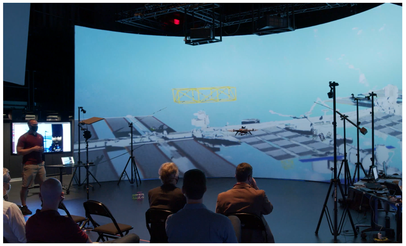
9. CUBE Theater Complex

The Virginia Tech CUBE [39] enables nearly 360 surround projection of pre-rendered or live synthetic environments on nine-foot high screens with very low shadow projection distances at a resolution of 1920 × 1200 at 13,000 lumens, effectively allowing for optical computer vision testing and development. Standing four stories high and consisting of 21,000 cubic meters of indoor space illustrated in Figure 25, this facility also allows large-scale system testing. By projecting the desired synthetic environment, we were able to repeatably and reliably test machine learning architectures in a physical space and then use that computer vision sensor data to manipulate real-world hardware within the same room—in our case, testing drone controls relative to an object of interest.

A wide range of rapidly augmentable synthetic worlds were designed to mimic optical sensor environments. We have endeavored to create a full end-to-end hardware-in-the-loop (HiL) testing facility for space application control, sensor, machine learning, and many other applications using free-flying robotics systems, allowing us to close the feedback loop between sensor perception, software interpolation, and hardware action and manipulation (as Figure 26 shows).

10. Results

10.1. Synthetic Data vs. Real World Results

To answer Research Question #1, “Can synthetic data be used for reliable real-world object tracking?”, synthetic ISS Imagery with associated truss sections was generated and compiled from the unreal engine into a training data set used to train the neural network, as described in the data set division section. The neural network will never see a real-world image during the training phase, only during testing. Real-world objects of interest are broken out into two different testing data sets. The first testing data set consists of imagery collected from real-world 3D-printed trusses, the identical trusses synthetically rendered and captured in the unreal engine. The second testing data set consists of solar panels collected and compiled in an orbital environment from several open-source databases, including NASA images and google images.

The ultimate goal of this method is to eliminate the need for real-world training imagery, solely or mostly relying on synthetic images. Thus, to form the basis of control, both synthetic imagery and real-world imagery data sets were evaluated against themselves in order to find the mean average precision performance within their own perspective domains.

Thus, evaluating a synthetic orbital environment data set against itself via the YOLO v5 Neural Network architecture results in an mAP(0.5) of 0.94 and mAP(0.5:0.95) of 0.77, respectively (Figure 27), which is extremely high performance. However, this performance is to be expected as there is a certain level of neural network memorization or overfitting that occurs when training within the confines of a very specific single-domain environment.

10.2. Real-World Data Base Tests

Evaluating the real-world truss data set against itself yielded an mAP(0.50) of 0.98 and mAP(0.5:0.95) of 0.90 (Figure 28), which is nearly perfect across all metrics, including precision, recall, and confidence. Ideally, all of the future CNNs will achieve this level of precision when evaluating the synthetic datasets and domain randomization methods below.

The resulting “F1” curve of the real-world a truss data set is displayed in Figure 29. The depiction on the left side is derived by combining both precision/confidence and recall/confidence curves into a single chart, as described in Equation (3). A greater area under the curve demonstrates better neural network performance. The resulting confusion matrix (shown on the right side) further breaks down the percentage of true positives (TPs), false positives (FPs), true negatives (TNs), and false negatives (FNs) for each class/object of interest. Numbers along the matrix diagonal indicate that an object is being identified correctly. Numbers outside the diagonal indicate a misclassification and subsequent loss in performance, either as another object or background. The bottom row represents background false negatives, while the last column represents background false positives. These metrics aid both researchers and observers to see where the CNN model is performing well and what areas are bringing down the overall network performance.

Due to the relatively large amount of imagery publicly available of solar panel systems currently deployed in orbit, real-world imagery was also evaluated against itself, yielding similar results of mAP(0.50) of 0.96 and mAP(0.5:0.95) of 0.78. This provides us with a real-world baseline when evaluating the use of synthetic imagery with real-world objects already in orbit.

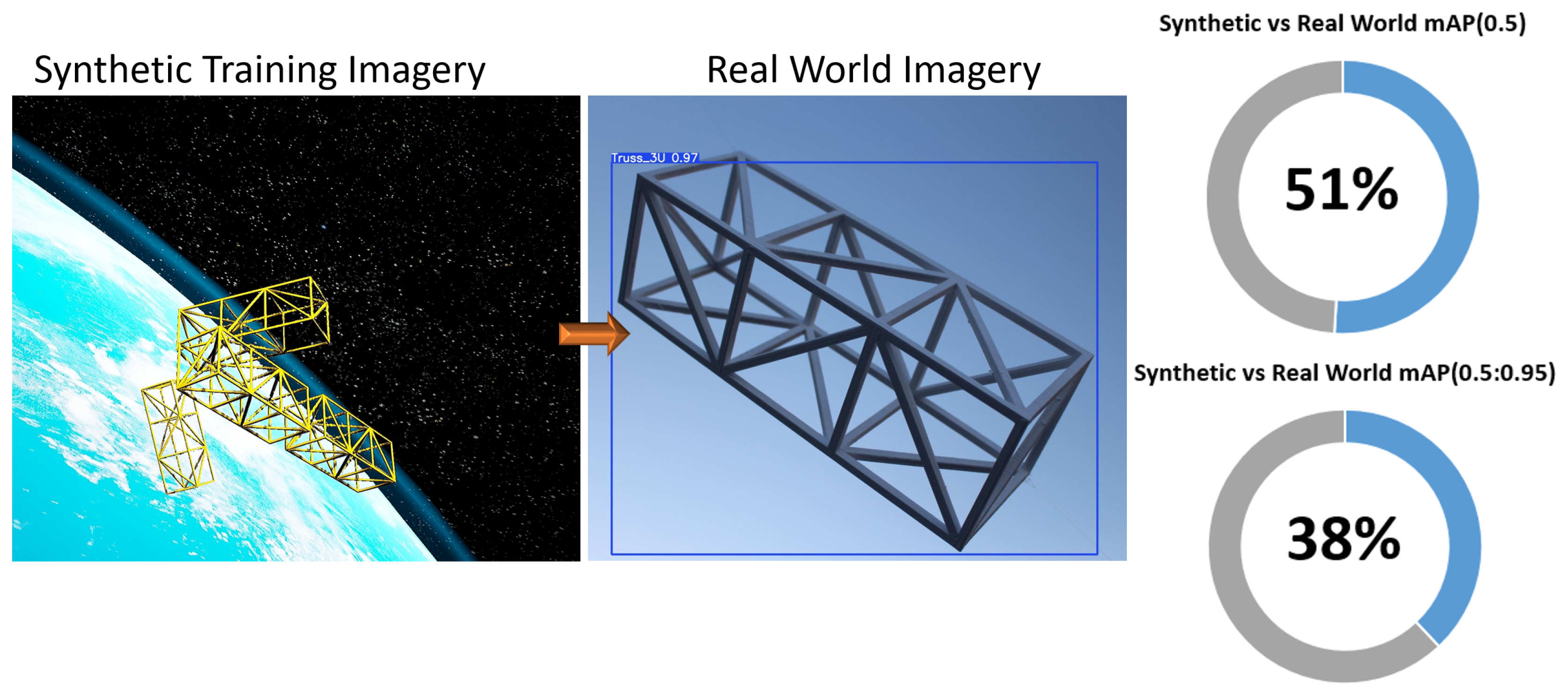
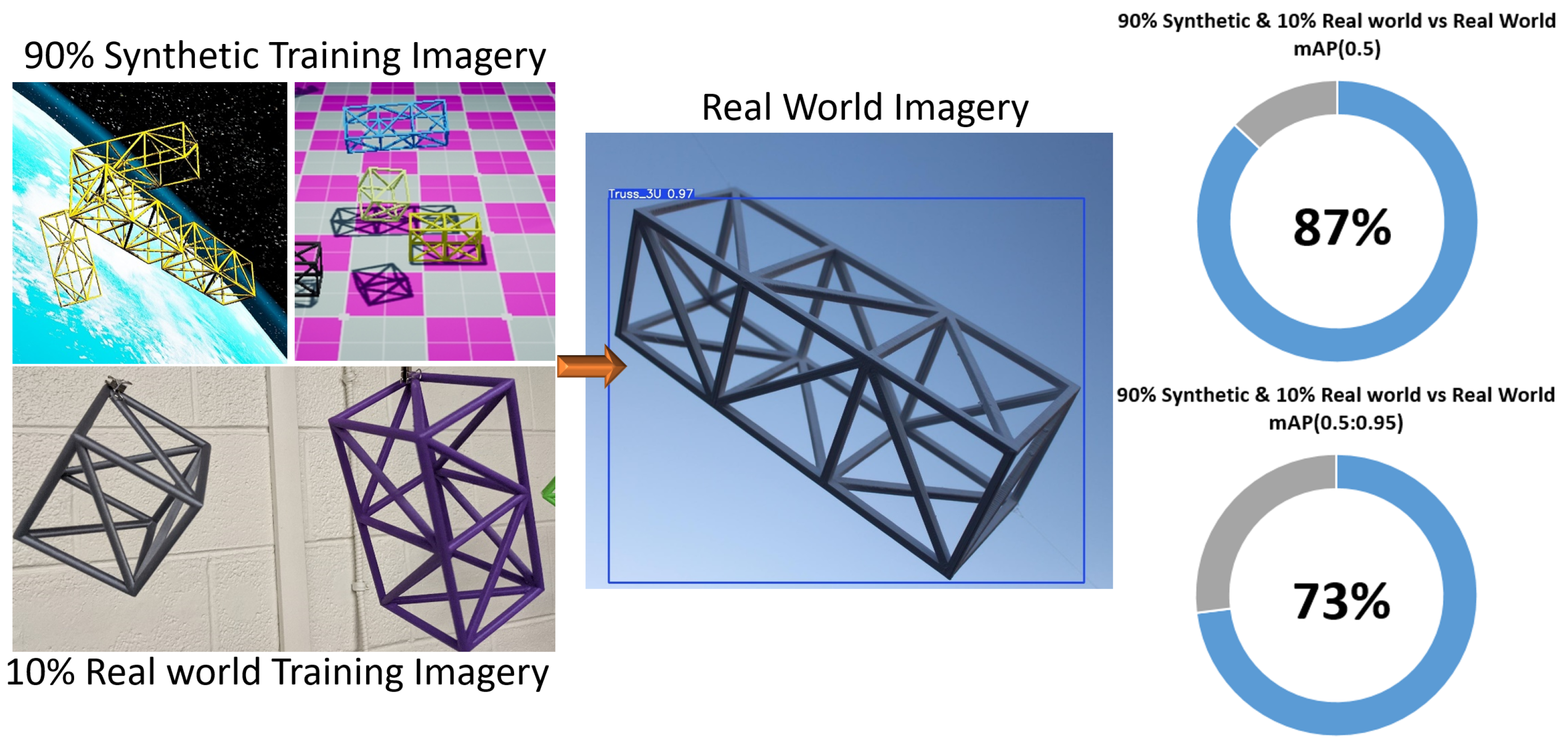
10.3. Synthetic Training vs. Real-World Results

With base case performance established within the synthetic and real-world domains, the next step is to determine if imagery from a synthetic domain can be used to train a network that can be applied to a real-world domain. Evaluating synthetically generated imagery of truss sections against real-world truss sections resulted in mAP(0.5) of 0.51 and mAP(0.5:0.95) of 0.38 (Figure 30). When compared to other results in computer science literature [40,41], these performance metrics may be deemed usable for other computer vision applications; however, given the high-risk operational environment, space agencies such as NASA, ESA, and SpaceX will more than likely require more robust and accurate models before entrusting major mission tasks to such an autonomous system. However, model performance can be improved further using the methods below. In order to reach an acceptable technology readiness level (TLR) and validation standards for the space industry, it is safe to assume that computer vision performance metrics will need to achieve higher precision. However, this is strictly an assumption. Given the relatively new nature of these applications in the aerospace industry, standards have not yet been established when compared to more mature technologies. This paper and others like it will start to develop these standards.

The same experiment was conducted evaluating a neural network trained on synthetic solar panels against real-world orbital solar panel imagery collected from open source repositories such as Google images. The experiment was far more favorable, yielding mAP(0.5) of 0.76 and mAP(0.5:0.95) of 0.69. Given the nonporous, uniform, and often similar color texture inherent to solar panel design, neural network transfer between the synthetic and real-world domains is much easier for this particular object of interest when compared to porous structures such as trusses or other types of construction scaffolding material. These results provide a real-world proof on concept for applying synthetically trained computer vision models directly to space applications with relatively high results.

The metric of mean average precision can be a little misleading by itself because it does not explain the capabilities of the model trained, only the confidence in a particular model when attempting to identify classes within a given frame (in this case, truss sections and solar panels). For example, mean average precision alone does not define if a model will perform well when alterations are made to the environment or object. These differences in model capability are often eliminated by evaluating models on standardized data sets, enabling a one-to-one comparison with other models. However, since standardized data sets for this space problem do not exist, direct comparisons are not possible. For example, non-standard objects of interest such as damaged, discolored, distorted, or an object not meeting manufacturing standards a computer vision model is trained to recognize will degrade any system’s ability to perform autonomous tasking. Introducing nonstandard structures, such as Figure 31, are often segmented or misclassified by traditionally trained computer vision models, especially if those models are transitioning across domains. Leveraging the domain randomization methods detailed below will also enable models that are more capable of correctly identifying these objects.

10.4. Domain Randomization Results

To make a more robust model to address some of the previously mentioned issues, we introduced domain randomized data sets into the CNN training. Using pre-rendered synthetic worlds, we introduce distractors, such as non-uniform truss sections, backgrounds, and lighting conditions, in a zero-gravity simulation environment at the preprocessing level. Introducing these domain randomized data sets into the YOLO v5 neural network architecture yielded an mAP(0.50) of 0.56 and an mAP(0.50:0.95) of 0.43, an increase of 5% for both perspective mAP metrics (Figure 32 and Figure 33). This performance increase shows that domain randomization can help bridge the reality gap when attempting to use synthetic optical imagery for real-world computer vision applications.

Domain randomized computer vision models are far more generalizable and capable of complex inferencing tasks, as shown in Figure 34, demonstrating reliable object detection regardless of color, light saturation, foreground, or background. This ability will be essential when a satellite or robotic platform repairing space infrastructure or exploring celestial bodies encounters a situation that it has not encountered before but can generalize and infer similar objects based on what it has been trained to see or do.

Finally, the foundation of this research assumes that a user has no imagery of the environment for which they are trying to train a computer vision architecture. However, to synthetically recreate an environment optically, at least some visual data must be gathered to form a starting block for a synthetic generation. Thus, what if a user has limited data of a particular environment? Can synthetic imagery fill in the gaps? To answer this question, we supplemented the purely synthetic training data set with real-world imagery at a ratio of 10% and then evaluated that new merged data set while ensuring that no real-world images were shared between the training and testing data sets. This small addition dramatically increased performance to mAP(0.50) of 0.87 and an mAP(0.50:0.95) of 0.73 (Figure 35), providing yet another data input solution to improve computer vision performance.

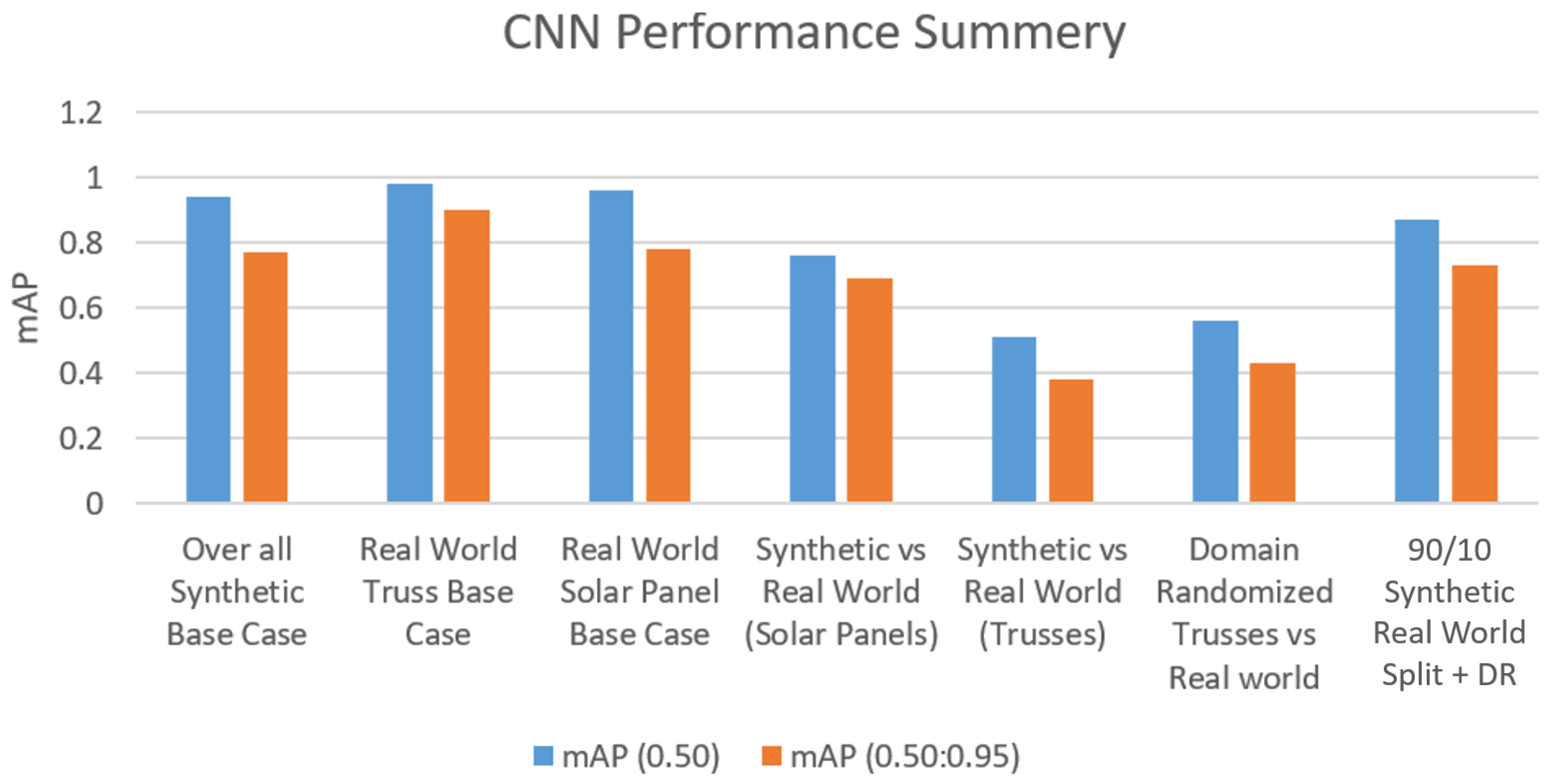
10.5. Computer Vision Results Summery

With results within 11% mAP(0.50) of a traditionally trained neural network utilizing 100% real-world imagery and within 4% mAP(0.50:0.95) of the synthetic baseline, summarized in

Table 1. Overall summery of all major neural network (YOLOv5) performance evaluations across data sets.

YOLO Neural Network Performance
Data Set (s)	mAP${}_{\mathbf{50}}$	mAP${}_{\mathbf{50}:\mathbf{95}}$
Overall Synthetic Base Case	94%	77%
Real world Truss Base Case	98%	90%
Real world Solar Panel Base Case	96%	78%
Synthetic vs. Real World (Solar Panel)	76%	69%
Synthetic vs. Real World (Trusses)	51%	38%
DR vs. Real World (Trusses)	56%	43%
90/10 Synthetic Real World split + DR	87%	73%

, domain randomized synthetic visual data are a viable solution for training a conventional neural network for real-world deployment if limited imagery data are available. Figure 36 summarizes computer vision performance starting with the three baseline performance metrics on the far left moving to the right, establishing cross-domain performance metrics for both solar panels and trusses, applying domain randomization and then applying both domain randomization (DR) and a 10% real-world data set to the training model.

Other works [40,41] have also employed mixed real-world/synthetic, as well as strictly synthetic, data sets to improve neural network performance by as much as 13% when applying domain randomization to the self-driving car computer vision problem. However, both of these studies had the advantage of evaluating against hundreds of thousands of images within the COCO [42] and VKITTI [43] data sets. As of today, a purpose-built data set of autonomous orbital tasking for computer vision training and testing does not exist other than perhaps Stanford’s SPEED data set [44] used for Spacecraft Pose Estimation. This paper provides an existing domain randomized orbital data set as well as the methodologies to generate and test new data sets for future applications.

Additionally, identifying geometrically similar objects across different sizes of SKUs (i.e., 1U, 2U, 3U trusses) is a significantly harder problem to solve when compared to simply identifying cars on a road surface. It is likely that construction elements for orbital assets and celestial habitats such as Mars will be made up of modular designs to simplify the process; thus, a computer vision architecture will need to be able to routinely tell the difference between similar parts during the assembly process.

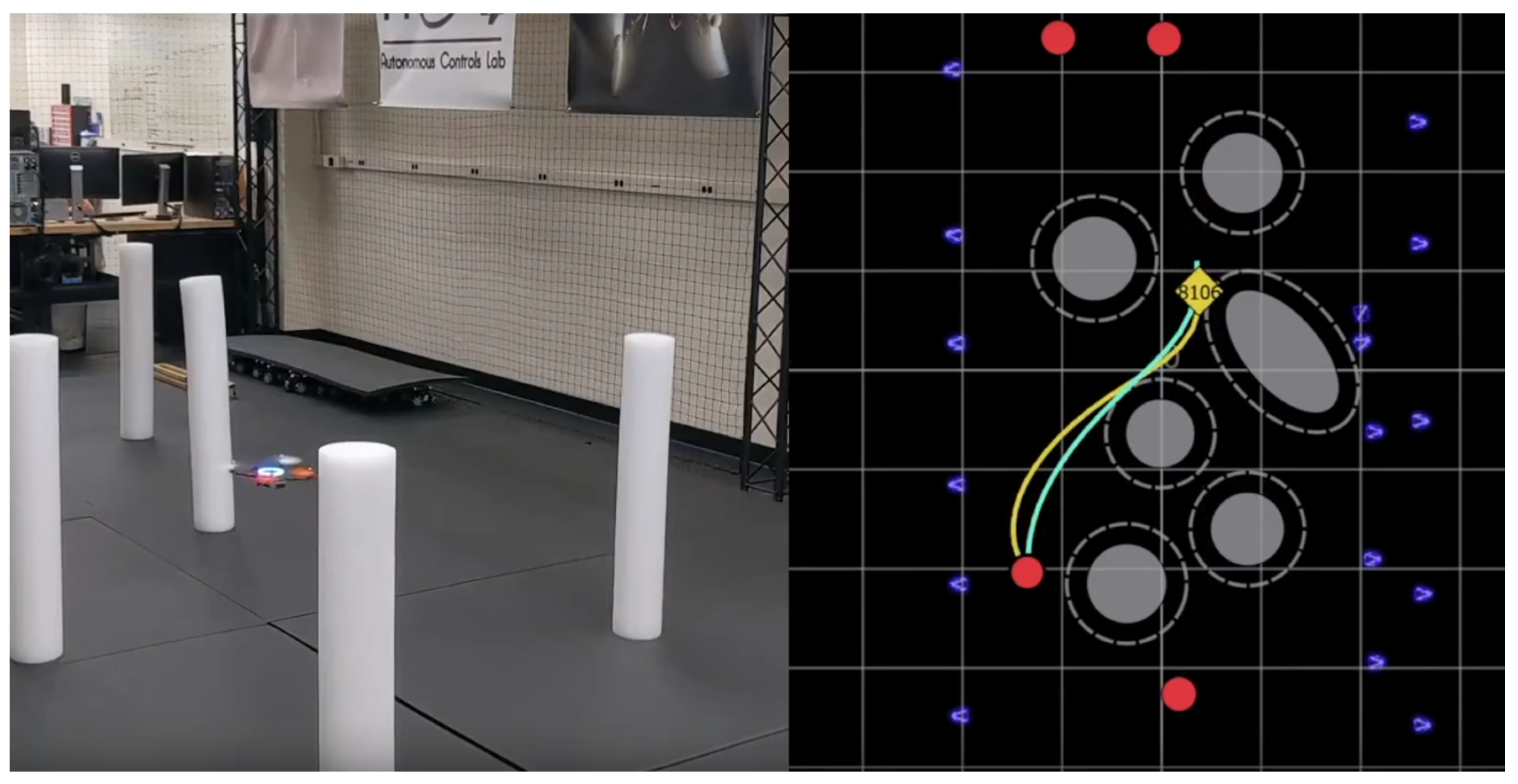
10.6. Localization and Robotic Arm Capture Results

Our localization method was tested in flight by scanning volume in the lab and returning the 3D localized positions of objects identified by the CNN. The results of this localization method are detailed in Figure 37. Identifying truss sections at 5 m results in an average 3D position error of 0.17 m in the direction of drone movement and 0.76 m in the perpendicular direction. Stationary error when both the camera/drone reference frame and object of interest are stationary is reduced to 0.26 m in the perpendicular axis.

Finally, by integrating the domain randomized solutions, we applied synthetically trained computer vision models for HIL application and testing. Using a sequence of dynamic and precise steps, we ultimately leverage neural networking, synthetic space domain environments, sensor integration, and robotics to lay the foundation for space-based HIL testing in the simulation at a price point that can be mass-produced and widely deployed. Using a synthetic environment of the user’s choice in the case of orbital truss sections in and around an existing space station, a SpaceDrone was deployed to perform autonomous pick-and-place operations solely using synthetically trained onboard RGB and LiDAR sensor data to perform real-time neural network inferencing to identify objects of interest. The capture sequence is initiated by maneuvering the drone to the proximity of the object, where the robotic arm is released from the stow position and inverse kinematics (IK) solutions drive the arm to the desired capture position at which point the end effector gripper is closed, completing the capture sequence. The object capture sequence is systematically accomplished via the following four steps illustrated in Figure 38 and detailed in Algorithm 1 below: (1) perform object classification and localization; (2) move closer to the object and deploy robotic arm for capture; (3) stow captured object for transport; (4) transport object to the desired location for release or placement. This capture sequence is better illustrated in video format below. (Video Link)

After the capture is complete, the object can be autonomously moved through space by any number of path planning optimization algorithms or other parameters set by the user.

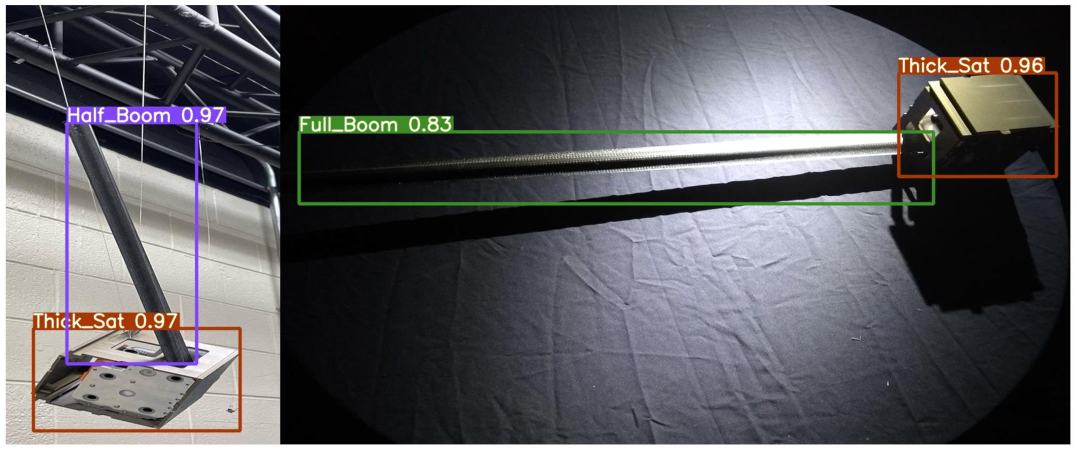
10.7. CUBE Computer Vision Results

All previous results and capabilities were integrated into a single hardware-in-the-loop simulation for optical/visual machine learning decision making, validation, and testing within the CUBE environment, as illustrated in Figure 26. The real-world mock-up models and objects were placed in the center, and the synthetic environment projected on the surrounding screens resulted in a unique optical visual simulation space. In regards to neural network performance, this simulation space resulted in a performance drop in the hybrid 90/10 CNN Model (synthetic/real-world) stack of only 4% and 5%, respectively, yielding an mAP(0.50) of 0.83 and an mAP(0.50:0.95) of 0.68 (

Table 2. Table of CUBE computer vision results.

YOLO Neural Network Performance
Data Set (s)	mAP${}_{\mathbf{50}}$	mAP${}_{\mathbf{50}:\mathbf{95}}$
CUBE Computer Vision Results	83%	68%

) at approximately 20 frames per second (FPS) in flight running on the Jetson Xavier board at a resolution of 640 × 360. The loss in performance is due to the inherent curvature of the screens not retaining true geometric proportions. However, training models within the CUBE that are robust to this simulation anomaly should render this a non-issue. The drone camera point of view (POV) during flight operations in the CUBE is shown in Figure 39. Drone flight video with onboard computer vision can be found at the following link (SpaceDrones CUBE Flight Video Link).

Algorithm 1 Sensor detection and Robotic Arm capture.

Require: Input for desired object

Conduct CNN object search

if CNN $confidence$ > 0.60 then

(x,y) object location = bounding box center

(z) object location = LiDAR point cloud of bounding box center

end if

if drone location ≠ Object location then

Maneuver drone to object of interest

end if

if drone location = Object location then

initiate robotic arm IK for object capture

if capture = True then

Stow captured object for transport

end if

end if

if capture = False then

Conduct CNN object search

re-initiate robotic arm IK for object capture

end if

The SpaceDrones visual simulation is also capable of simulating other deep space environments such as Mars to test vision-based autonomous habitat design, assembly, and inspection. Synthetically generated environments projected in the Virginia Tech Cube are illustrated in Figure 40. The bottom picture illustrates a real-world drone being mirrored as a virtual reality drone within the Unreal Engine. Porting position data of real-world and virtual objects to and from synthetic environments allow researchers to attempt testing on relatively dangerous operations using real-world hardware without risking damage to a vehicle when motion is projected in synthetic space. A video of this process is illustrated in the following video link (SpaceDrones VR Projection video link).

11. Discussion

This research has demonstrated the ability to use infinitely adjustable synthetic world creation tools to generate synthetic training data for a computer vision architecture. These trained CV models were then deployed onboard mobile manipulation drone platforms complete with sensor integration APIs for the purpose of autonomous tasking and object capture using mostly COTS compute hardware. This free-flying drone capability was then successfully deployed in a uniquely capable synthetic environment projected within a real-world space using large-scale theater technologies, demonstrating a hardware-in-the-loop testing methodology to evaluate onboard computer vision and drone control for a wide range of environments, including dynamic orbital environments. Further domain randomization of these synthetic worlds was used to bridge the reality gap between synthetically trained computer vision models and real-world target domains that these systems will ultimately be deployed to. To my knowledge, this is the first study to integrate computer vision, domain randomization, environmental projection, and free-flying mobile manipulation platforms into a complete end-to-end solution. At the time of this publication, the current computer vision simulation capability meets the NASA Technology Readiness Level 5 (TRL5) specifications, with the Virginia Tech Cube providing component validation within a relevant environment. HIL simulation and testing to include both the drone platform and robotic arm are TLR4, capable of verification in a laboratory environment. For spaceborne applications, a full 6DOF motion must be achieved before it can be considered a “relevant environment”. The readiness level will only increase as the future work capabilities detailed in the following section are implemented. As one can imagine, this capability is not limited to space applications but to any project in need of real-time onboard detection of large numbers of heterogeneous objects or in need of a flying sensor platform for system testing and autonomous tasking.

12. Contributions

This body of work is unique and holistic in its design to test and ultimately implement machine learning architectures into a complex space domain. The contributions of this work are listed below:

• The introduction of several thousand labeled synthetic and real-world orbital data sets available here [45];
• Ready made synthetic worlds and domain randomization tools for orbital/deep space environments available here [35];
• To our knowledge, it is the world’s first application of pre-processed domain randomized imagery for space-based machine learning tasks;
• Real-time hardware-in-the-loop optical testing environment for computer vision systems inside a projection space such as the Virginia Tech CUBE [39];
• Real-time machine learning, computer vision, and robotics integration of all the above-mentioned contributions on-board a flying drone testbed platform to further implement and test such capabilities.

13. Conclusions

This capability requires a working knowledge of several different disciplines, including software engineering, robotics, computer vision, machine learning, fabrication, animation, theater projection, and visual design—all culminating in a successful deployment of automated robotic tasking and object capture/manipulation via onboard computer vision and sensor localization. This dissertation has demonstrated the applicability of Convolutional Neural Networks, synthetic data generation, and domain randomization to detect various orbital objects of interest for In-Space Assembly (ISA) On-Orbit servicing (OOS) operations in simulated environments, achieving a mean average precision within 11% of non-synthetically trained models for a rather difficult array of geometrically similar objects. The simulated environment was then pulled out of a relatively small computer screen and projected onto a large 21,000-cubic-meter space for large-scale visual simulation, thus enabling researchers to interact with real-world hardware within a virtual environment. This solution has opened the door for hardware-in-the-loop computer vision testing onboard a real-world free flying hardware in environments that are difficult to capture or recreate or safely operating hardware in a controlled testing regime. This system will only continue to improve as more capabilities (detailed below in the future work section) are brought online. However, the problem of hardware-in-the-loop testing for any number of parameters or environmental factors is not specific to the aerospace community. This simulation solution can be applied to any number of research areas, including search and rescue, defense, and general automation applications. A short video detailing this projects methodologies in chronological order can be found at (SpaceDrones 2.0 Video Summary).

14. Future Work

This project was not developed in a vacuum, but it was designed to be integrated into a larger space domain awareness simulation and testing suite. The system can achieve 4DOF virtual simulation with a constant downward gravity vector, which effectively couples pitch and roll motion with translation. In an effort to simulate uncoupled 6DOF motion, a sister lab is developing an omni-directional drone platform [46,47] known as the “Omnicopter”, as illustrated in Figure 41. This 6DOF platform emulating orbital motion will provide a highly capable HIL simulation platform. Additionally, we aim to simulate frictionless motion similar to an air-bearing table via drone PID controllers. Such capabilities will enable true 6DOF HIL testing for space application when paired with a facility, such as the Virginia Tech CUBE.

Additionally, path planning is an essential part of autonomous tasks. Organizations such as the University of Washington’s Autonomous Control Laboratory have achieved high fidelity drone control and path planning architecture [48,49]. An example of such a system is illustrated in Figure 42. Implementing these capabilities into the existing SpaceDrones architecture is currently in development and is a high priority for future operations.

Lastly, this experiment was also expanded to a real-world small satellite, currently in the process of being deployed by the Virginia Tech satellite team (See Figure 43). This particular satellite has a spring-loaded boom that is designed to extend once it reaches orbit. If this particular boom does not extend to its full length, it is classified as a failed state. Determining whether or not the boom has failed and other satellite related failures purely using Computer Vision is another experimental result that can be further expanded upon in the future work.

References

1. Hoyt, R.P. SpiderFab: An architecture for self-fabricating space systems. In Proceedings of the AIAA SPACE 2013 Conference and Exposition, San Diego, CA, USA, 10–12 September 2013; p. 5509. [Google Scholar]
2. Jairala, J.C.; Durkin, R.; Marak, R.J.; Sipila, S.A.; Ney, Z.A.; Parazynski, S.E.; Thomason, A.H. EVA Development and Verification Testing at NASA’s Neutral Buoyancy Laboratory. In Proceedings of the 42nd International Conference on Environmental Systems (ICES), San Diego, CA, USA, 15–19 July 2012; No. JSC-CN-26179. [Google Scholar]
3. Zero Gravity Research Facility—Glenn Research Center. NASA. Available online: https://www1.grc.nasa.gov/facilities/zero-g/ (accessed on 17 March 2020).
4. Daryabeigi, K. Thermal Vacuum Facility for Testing Thermal Protection Systems; National Aeronautics and Space Administration, Langley Research Center: Hampton, VA, USA, 2002. [Google Scholar]
5. Christensen, B.J.; Gargioni, G.; Doyle, D.; Schroeder, K.; Black, J. Space Simulation Overview: Leading Developments towards using Multi-Rotors to Simulate Space Vehicle Dynamics. In Proceedings of the AIAA Scitech 2020 Forum, Orlando, FL, USA, 6–10 January 2020; p. 1134. [Google Scholar]
6. D’Amico, S.; Eddy, D.; Makhadmi, I. TRON—The Testbed for Rendezvous and Optical Navigation—Enters the Grid; Space Rendezvous Laboratory: Stanford, CA, USA, 2016. [Google Scholar]
7. Oestreich, C.; Lim, T.W.; Broussard, R. On-Orbit Relative Pose Initialization via Convolutional Neural Networks. In Proceedings of the AIAA Scitech 2020 Forum, Orlando, FL, USA, 6–10 January 2020. [Google Scholar]
8. Scharf, D.P.; Hadaegh, F.Y.; Keim, J.A.; Benowitz, E.G.; Lawson, P.R. Flight-like ground demonstration of precision formation flying spacecraft. Proc. SPIE 2007, 6693, 669307. [Google Scholar] [CrossRef]
9. Trigo, G.F.; Maass, B.; Krüger, H.; Theil, S. Hybrid optical navigation by crater detection for lunar pin-point landing: Trajectories from helicopter flight tests. CEAS Space J. 2018, 10, 567–581. [Google Scholar] [CrossRef] [Green Version]
10. Enright, J.; Hilstad, M.; Saenz-Otero, A.; Miller, D. The SPHERES guest scientist program: Collaborative science on the ISS. In Proceedings of the 2004 IEEE Aerospace Conference Proceedings (IEEE Cat. No. 04TH8720), Big Sky, MT, USA, 6–13 March 2004; Volume 1. [Google Scholar]
11. Sharma, S.; Ventura, J.; D’Amico, S. Robust model-based monocular pose initialization for noncooperative spacecraft rendezvous. J. Spacecr. Rockets 2018, 55, 1414–1429. [Google Scholar] [CrossRef] [Green Version]
12. Thomas, D.; Kelly, S.; Black, J. A monocular SLAM method for satellite proximity operations. In Proceedings of the 2016 American Control Conference (ACC), Boston, MA, USA, 6–8 July 2016; pp. 4035–4040. [Google Scholar] [CrossRef]
13. Mark, C.P.; Kamath, S. Review of active space debris removal methods. Space Policy 2019, 47, 194–206. [Google Scholar] [CrossRef]
14. Peng, H.; Bai, X. Improving orbit prediction accuracy through supervised machine learning. Adv. Space Res. 2018, 61, 2628–2646. [Google Scholar] [CrossRef] [Green Version]
15. Li, S.; Lu, R.; Zhang, L.; Peng, Y. Image Processing Algorithms For Deep-Space Autonomous Optical Navigation. J. Navig. 2013, 66, 605–623. [Google Scholar] [CrossRef] [Green Version]
16. Petkovic, M.; Lucas, L.; Kocev, D.; Džeroski, S.; Boumghar, R.; Simidjievski, N. Quantifying the effects of gyroless flying of the mars express spacecraft with machine learning. In Proceedings of the 2019 IEEE International Conference on Space Mission Challenges for Information Technology (SMC-IT), Pasadena, CA, USA, 30 July–1 August 2019; pp. 9–16. [Google Scholar]
17. Fang, H.; Shi, H.; Dong, Y.; Fan, H.; Ren, S. Spacecraft power system fault diagnosis based on DNN. In Proceedings of the 2017 Prognostics and System Health Management Conference (PHM-Harbin), Harbin, China, 9–12 July 2017; pp. 1–5. [Google Scholar] [CrossRef]
18. Rubinsztejn, A.; Sood, R.; Laipert, F.E. Neural network optimal control in astrodynamics: Application to the missed thrust problem. Acta Astronaut. 2020, 176, 192–203. [Google Scholar] [CrossRef]
19. Shirobokov, M.; Trofimov, S.; Ovchinnikov, M. Survey of machine learning techniques in spacecraft control design. Acta Astronaut. 2021, 186, 87–97. [Google Scholar] [CrossRef]
20. Izzo, D.; Märtens, M.; Pan, B. A survey on artificial intelligence trends in spacecraft guidance dynamics and control. Astrodynamics 2019, 3, 287–299. [Google Scholar] [CrossRef]
21. Jocher, G. ultralytics/yolov5: v3.1—Bug Fixes and Performance Improvements. 2020. Available online: https://github.com/ultralytics/yolov5 (accessed on 5 April 2022). [CrossRef]
22. Tobin, J.; Fong, R.; Ray, A.; Schneider, J.; Zaremba, W.; Abbeel, P. Domain randomization for transferring deep neural networks from simulation to the real world. In Proceedings of the 2017 IEEE/RSJ international conference on intelligent robots and systems (IROS), Vancouver, BC, Canada, 24–28 September 2017; pp. 23–30. [Google Scholar]
23. Girshick, R. Fast R-CNN. arXiv 2015, arXiv:cs.CV/1504.08083. [Google Scholar]
24. Dai, J.; Li, Y.; He, K.; Sun, J. R-FCN: Object Detection via Region-based Fully Convolutional Networks. arXiv 2016, arXiv:cs.CV/1605.06409. [Google Scholar]
25. Boone, B.; Bruzzi, J.; Dellinger, W.; Kluga, B.; Strobehn, K. Optical simulator and testbed for spacecraft star tracker development. In Optical Modeling and Performance Predictions II. International Society for Optics and Photonics; SPIE: Bellingham, WA, USA, 2005; Volume 5867, p. 586711. [Google Scholar]
26. Krizhevsky, A.; Sutskever, I.; Hinton, G.E. ImageNet Classification with Deep Convolutional Neural Networks. Commun. ACM 2017, 60, 84–90. [Google Scholar] [CrossRef]
27. Lebreton, J.; Brochard, R.; Baudry, M.; Jonniaux, G.; Salah, A.H.; Kanani, K.; Goff, M.L.; Masson, A.; Ollagnier, N.; Panicucci, P.; et al. Image simulation for space applications with the SurRender software. arXiv 2021, arXiv:2106.11322. [Google Scholar]
28. Ren, S.; He, K.; Girshick, R.; Sun, J. Faster R-CNN: Towards Real-Time Object Detection with Region Proposal Networks. arXiv 2016, arXiv:cs.CV/1506.01497. [Google Scholar] [CrossRef] [Green Version]
29. Lin, T.Y.; Goyal, P.; Girshick, R.; He, K.; Dollár, P. Focal Loss for Dense Object Detection. arXiv 2018, arXiv:cs.CV/1708.02002. [Google Scholar]
30. Wang, J.; Chen, K.; Yang, S.; Loy, C.C.; Lin, D. Region Proposal by Guided Anchoring. arXiv 2019, arXiv:cs.CV/1901.03278. [Google Scholar]
31. Goodfellow, I.J.; Pouget-Abadie, J.; Mirza, M.; Xu, B.; Warde-Farley, D.; Ozair, S.; Courville, A.; Bengio, Y. Generative Adversarial Networks. arXiv 2014, arXiv:stat.ML/1406.2661. [Google Scholar] [CrossRef]
32. Srivastava, N.; Hinton, G.; Krizhevsky, A.; Sutskever, I.; Salakhutdinov, R. Dropout: A simple way to prevent neural networks from overfitting. J. Mach. Learn. Res. 2014, 15, 1929–1958. [Google Scholar]
33. Ye, C.; Evanusa, M.; He, H.; Mitrokhin, A.; Goldstein, T.; Yorke, J.A.; Fermüller, C.; Aloimonos, Y. Network Deconvolution. arXiv 2020, arXiv:cs.LG/1905.11926. [Google Scholar]
34. Bochkovskiy, A.; Wang, C.Y.; Liao, H.Y.M. YOLOv4: Optimal Speed and Accuracy of Object Detection. arXiv 2020, arXiv:2004.10934. [Google Scholar]
35. Peterson, M.; Du, M. SpaceDrones Unreal Engine Projects; Virginia Tech Library: Blacksburg, VA, USA, 2022. [Google Scholar] [CrossRef]
36. Gargioni, G.; Peterson, M.; Persons, J.; Schroeder, K.; Black, J. A full distributed multipurpose autonomous flight system using 3D position tracking and ROS. In Proceedings of the 2019 International Conference on Unmanned Aircraft Systems (ICUAS), Atlanta, GA, USA, 11–14 June 2019; pp. 1458–1466. [Google Scholar]
37. Quigley, M.; Conley, K.; Gerkey, B.; Faust, J.; Foote, T.; Leibs, J.; Wheeler, R.; Ng, A.Y. ROS: An open-source Robot Operating System. In Proceedings of the ICRA Workshop on Open Source Software, Kobe, Japan, 12–17 May 2009; Volume 3, p. 5. [Google Scholar]
38. Du, M.; Gargioni, G.; Peterson, M.A.; Doyle, D.; Black, J. IR based local tracking system Assessment for planetary exploration missions. In Proceedings of the ASCEND 2020, Virtual Event, 16–18 November 2020. [Google Scholar] [CrossRef]
39. Lyon, E.; Caulkins, T.; Blount, D.; Ico Bukvic, I.; Nichols, C.; Roan, M.; Upthegrove, T. Genesis of the cube: The design and deployment of an hdla-based performance and research facility. Comput. Music J. 2016, 40, 62–78. [Google Scholar] [CrossRef]
40. Tremblay, J.; Prakash, A.; Acuna, D.; Brophy, M.; Jampani, V.; Anil, C.; To, T.; Cameracci, E.; Boochoon, S.; Birchfield, S. Training deep networks with synthetic data: Bridging the reality gap by domain randomization. In Proceedings of the IEEE Conference on Computer Vision and Pattern Recognition Workshops, Salt Lake City, UT, USA, 18–22 June 2018; pp. 969–977. [Google Scholar]
41. Yue, X.; Zhang, Y.; Zhao, S.; Sangiovanni-Vincentelli, A.; Keutzer, K.; Gong, B. Domain randomization and pyramid consistency: Simulation-to-real generalization without accessing target domain data. In Proceedings of the IEEE/CVF International Conference on Computer Vision, Seoul, Korea, 27 October–2 November 2019; pp. 2100–2110. [Google Scholar]
42. Lin, T.Y.; Maire, M.; Belongie, S.; Bourdev, L.; Girshick, R.; Hays, J.; Perona, P.; Ramanan, D.; Zitnick, C.L.; Dollár, P. Microsoft COCO: Common Objects in Context. arXiv 2015, arXiv:cs.CV/1405.0312. [Google Scholar]
43. Geiger, A.; Lenz, P.; Stiller, C.; Urtasun, R. Vision meets Robotics: The KITTI Dataset. Int. J. Robot. Res. (IJRR) 2013, 32, 1231–1237. [Google Scholar] [CrossRef] [Green Version]
44. Sharma, S.; D’Amico, S. Pose Estimation for Non-Cooperative Rendezvous Using Neural Networks. arXiv 2019, arXiv:cs.CV/1906.09868. [Google Scholar]
45. Peterson, M. SpaceDrones Labeled Training Images and Results; Virginia Tech Library: Blacksburg, VA, USA, 2022. [Google Scholar] [CrossRef]
46. Deans, C.; Furgiuele, T.; Doyle, D.; Black, J. Simulating Omni-Directional Aerial Vehicle Operations for Modeling Satellite Dynamics. In Proceedings of the ASCEND 2020, Virtual Event, 16–18 November 2020; p. 4023. [Google Scholar] [CrossRef]
47. Blandino, T.; Leonessa, A.; Doyle, D.; Black, J. Position Control of an Omni-Directional Aerial Vehicle for Simulating Free-Flyer In-Space Assembly Operations. In Proceedings of the ASCEND 2021, Las Vegas, NV, USA, 15–17 November 2021; p. 4100. [Google Scholar] [CrossRef]
48. Yu, Y.; Elango, P.; Topcu, U.; Açıkmeşe, B. Proportional-Integral Projected Gradient Method for Conic Optimization. arXiv 2021, arXiv:2108.10260. [Google Scholar]
49. Yu, Y.; Topcu, U. Proportional-Integral Projected Gradient Method for Infeasibility Detection in Conic Optimization. arXiv 2021, arXiv:2109.02756. [Google Scholar]
Figure 1. Manned crew performing maintenance operation on the Hubble Telescope (Left); SpiderFab orbital assembly render concept [1] (Top Right); on-orbit serving render concept (Bottom Right).
Aerospace 09 00254 g001
Figure 2. Stanford TRON testbed - Space Rendezvous Laboratory (SLAB) citeTRON (Top Left); United States Naval Academy attitude initialization study [7] (Top Right); 2D air bearing autonomous spacecraft testing of robotic operations in space [8] (Bottom Left); German Aerospace Center optical navigation via moon crater detection [9] (Bottom Right).
Aerospace 09 00254 g002
Figure 3. Synthetic creation, domain randomization, and evaluation or orbital environments for space-based computer vision applications.
Aerospace 09 00254 g003
Figure 4. Deployment of the previously mentioned synthetically trained computer vision model onboard a free-flying drone, which is then deployed to a theater projection workspace for hardware-in-the-loop development, testing, and evaluation of vision-based autonomous tasking.
Aerospace 09 00254 g004
Figure 5. Synthetic render of the James Webb Telescope (JWST) in Unreal Engine 5 using the same synthetic generation methods described in this paper.
Aerospace 09 00254 g005
Figure 6. Simplified neural network architecture diagram using synthetic images as input, resulting in object classification.
Aerospace 09 00254 g006
Figure 7. Example of synthetic orbital images generated using Unreal Engine 4.
Aerospace 09 00254 g007
Figure 8. Example domain randomization images generated using Unreal Engine 4 (Video Link).
Aerospace 09 00254 g008
Figure 9. Project work flow for CAD and STL Files.
Aerospace 09 00254 g009
Figure 10. Division of imagery data between real-world and synthetic sources.
Aerospace 09 00254 g010
Figure 11. Pixhawk to Xavier NX GPIO Pin out.
Aerospace 09 00254 g011
Figure 12. SpaceDrones VR system tracking and control architecture.
Aerospace 09 00254 g012
Figure 13. RGB Camera and LiDAR Point cloud senor data side-by-side.
Aerospace 09 00254 g013
Figure 14. Drone Localization and Capture Software Diagram.
Aerospace 09 00254 g014
Figure 15. Porous structure LiDAR point cloud problem and solution.
Aerospace 09 00254 g015
Figure 16. Drone chassis and integrated systems render.
Aerospace 09 00254 g016
Figure 17. Drone world frame to camera frame offset.
Aerospace 09 00254 g017
Figure 18. Drone L515 Camera inertial frame position offset.
Aerospace 09 00254 g018
Figure 19. Drone L515 camera inertial frame rotation offset.
Aerospace 09 00254 g019
Figure 20. Target inertial frame rotation with respect to the drone.
Aerospace 09 00254 g020
Figure 21. Drone Arm link measurements (mm).
Aerospace 09 00254 g021
Figure 22. Drone arm base frame relative to other world frames.
Aerospace 09 00254 g022
Figure 23. Depiction of the integrated drone, camera, and robotic arm system.
Aerospace 09 00254 g023
Figure 24. RGB computer vision during sensor saturation events.
Aerospace 09 00254 g024
Figure 25. Physical-virtual hardware-in-the-loop simulation solution at Virginia Tech CUBE.
Aerospace 09 00254 g025
Figure 26. Onboard drone computer vision testing inside a physical/virtual simulation projection at Virginia Tech’s CUBE facility.
Aerospace 09 00254 g026
Figure 27. Synthetic orbital data set self evaluation results showing relatively high mean average precision (mAP) over 250 training epochs, establishing a baseline performance metric.
Aerospace 09 00254 g027
Figure 28. Real-world truss data set self evaluation results showing relatively high mean average precision (mAP) over 250 training epochs, establishing a baseline performance metric.
Aerospace 09 00254 g028
Figure 29. Real-world truss data set self evaluation: F1 curve (left); confusion matrix (right).
Aerospace 09 00254 g029
Figure 30. Mean average precision result when training with synthetic imagery and testing against real-world imagery.
Aerospace 09 00254 g030
Figure 31. Non-standard trusses used to evaluate neural network performance before and after introducing domain randomization: 2U Truss (Left); 3U Trusses (Middle and Right).
Aerospace 09 00254 g031
Figure 32. Domain randomized synthetic data set self evaluation: F1 curve (left); confusion matrix (right).
Aerospace 09 00254 g032
Figure 33. Mean average precision result when training with domain randomized synthetic imagery and testing against real-world imagery.
Aerospace 09 00254 g033
Figure 34. Domain randomized vs. non-domain randomized results.
Aerospace 09 00254 g034
Figure 35. Mean average precision result when trained 90% domain randomized synthetic imagery and 10% real-world imagery evaluated against a real-world data set.
Aerospace 09 00254 g035
Figure 36. Overall summery of all major neural network (YOLOv5) performance evaluations across data sets. Synthetic imagery can achieve results within 11% mAP(0.50) of real-world base lines and within 4% mAP(0.50:0.95) of baseline metrics.
Aerospace 09 00254 g036
Figure 37. Five-meter LiDAR scan localization result when integrating computer vision bounding box data with LiDAR point cloud data.
Aerospace 09 00254 g037
Figure 38. Chronological illustration of drone pick sequence (Video Link).
Aerospace 09 00254 g038
Figure 39. Drone camera POV (point of view) running computer vision on objects of interest against a synthetic orbital background (Video Link).
Aerospace 09 00254 g039
Figure 40. Simulated Mars environment with virtual reality drone bodies performing autonomous tasking (Top). Mars environment projection in the Virginia Tech Cube with real-world drone motioned being mirrored to a virtual drone vehicle (Bottom), (Video Link).
Aerospace 09 00254 g040
Figure 41. Virginia Tech Omni-directional drone (Omnicopter).
Aerospace 09 00254 g041
Figure 42. Vehicle path planning by the University of Washington’s Autonomous Control Laboratory [48].
Aerospace 09 00254 g042
Figure 43. Full vs. half-boom extension using computer vision to determine deployment failures on real-world spaceflight hardware.
Aerospace 09 00254 g043