Abstract
This paper proposes a modified glideslope guidance method that optimizes a hybrid multiobjective of bearing-only navigation error and fuel consumption. The traditional glideslope guidance fixes uniform maneuver intervals and the initial approach velocity as a predetermined value, making this approach inflexible. In this paper, the maneuver intervals and the initial approach velocity were used as optimization variables, and a hybrid cost function was designed. The tradeoff between the two objectives was analyzed with a bearing-only navigation simulation conducted to reveal the navigation performance following different resulting trajectories. The result showed that the optimal scheduled times of maneuvers remained relatively stable under different tradeoff weights, while a strong correlation between the optimal initial approach velocity and the tradeoff weight was revealed. Therefore, when the optimization has to be solved several times online with different tradeoff weights, the initial approach velocity can be the only optimization variable, leaving the scheduled times of maneuvers fixed in the optimal values achieved offline. These findings provide a potential reference for far-approach trajectory design of bearing-only navigation.
1. Introduction
Small celestial body missions are popular with different mission profiles, such as impactors [1], high-speed flybys [2], orbiters [3], landers [4], and sample returns [5,6,7], because they cannot only promote space technology to defend the Earth, but also help us understand the origin and evolution of the solar system [8].
The far-approach phase is necessary for all small celestial body missions [9,10]. It is the key phase where the interplanetary transfer ends and the detection of the asteroid begins [11]. Due to the orbit propagation error and the maneuver execution error during the interplanetary transfer phase, as well as the error of the asteroid ephemeris, far-approach guidance is necessary to arrive at a relative range and accuracy that will allow the start of close-approach autonomous operations.
The far-approach guidance of the spacecraft usually realizes the optimization of some performance indices (such as fuel consumption or rendezvous time) under multiple constraints. This generally requires that the original problem to be constructed as an optimal control problem (OCP), such as linear programming (LP), quadratic programming (QP), quadratically constrained quadratic programming (QCQP), second-order cone programming (SOCP), and mixed integer programming (MIP) [12,13,14]. These problems are generally solved by the active set or interior point method [3]. Due to the high sensitivity of open-loop rendezvous guidance in the face of uncertain conditions, autonomous guidance generally requires such an optimal control problem to be embedded into the closed-loop feedback system, in which the real-time estimation of the state by the navigation system is used as the input of the closed-loop guidance. In the closed-loop feedback guidance architecture, the optimal control problem needs to be solved repeatedly with a receding time horizon and using current navigation filter estimates to set the initial conditions (ICs) for the optimization, which corresponds to model predictive control in spacecraft rendezvous [15]. This puts forward high requirements for computational efficiency when repeatedly solving the optimal control problem. In addition, Hablani proposed a multipulse glideslope guidance method based on the Clohessy–Wiltshire (CW) equation [16], which was used for rendezvous and proximity operations of the Space Shuttle because of its advantages of an arbitrary design of the approximation direction, gradual reduction of the relative distance and relative speed, prevention of collision, and safety. However, these guidance methods usually fix uniform maneuver intervals and do not consider the optimization of the scheduled times of maneuvers. Benedikter discretizes the independent variable over a dense time grid to optimize the scheduled times of maneuvers, which is a viable choice, despite one that makes the problem more complex [17].
In recent years, some researchers have taken navigation performance into consideration in guidance method design [18]. During the far-approach phase to a small celestial body, the spacecraft is far from the body, and the available relative measurement sensor is generally only a narrow field camera. Therefore, the uniqueness of the asteroid far-approach guidance design lies in the fact that the limited available sensors necessitate the observability and navigation accuracy of relative angle-only navigation (AON) [19]. Based on the geometric interpretation of maneuvers in angle-only rendezvous, Woffinden and Geller proposed observability criteria for AON and developed an analytical solution of the maneuver for optimizing observability [19,20]. Subsequently, Grzymisch et al. derived a simpler closed form of the observability criteria from the concept of linear uncorrelation, analytically obtained optimal observability maneuvers and proposed an optimal rendezvous guidance method with enhanced angle-only observability [18,21,22]. Mok et al. defined an observability measurement derived from the Fisher information matrix (FIM) and the Cramér–Rao lower bound (CRLB) and added this measurement to the optimization objective function to obtain a multipulse rendezvous guidance law [23]. Based on an angle-only measurement equation with pseudorange measurement, Hou et al. used the FIM and the CRLB to estimate navigation accuracy, providing another observability criterion. The sum of the CRLB at each observation time during the whole process was taken as the objective function of single maneuver rendezvous optimization [24]. In addition to theoretical research, an angle-only rendezvous on-orbit test was conducted at the end of the PRISMA mission [25]. In this test, the orbit maneuver of the spacecraft was planned offline to maintain the desired formation configuration, and observability was used to select a better strategy from the solved rendezvous strategy set. Generally, the above studies also fix uniform maneuver intervals. They are suitable for missions with short rendezvous times [26].
In our work, navigation accuracy optimization, fuel consumption optimization, and multipulse glideslope guidance are combined to realize a multipulse glideslope guidance method with an enhanced navigation accuracy. The scheduled times of maneuvers and the initial approach velocity are used as optimization variables to reveal their influence on the far approach guidance. The proposed method retains the advantages of the multipulse glideslope guidance method, including on-demand approach direction design and the decreasing approach speed with the distance, and adds the optimization of the mixed index of AON accuracy and fuel consumption. It is an attractive choice for the approach trajectory design of a small celestial body mission.
The structure of this paper is organized as follows. First, the navigation accuracy criteria based on the FIM are given in Section 2. Then, Section 3 introduces traditional multipulse glideslope guidance and analyzes its potential independent variables. In Section 4, an offline multipulse glideslope guidance method with a hybrid optimization of the navigation accuracy and fuel consumption is proposed. Then, simulation results are given in Section 5, and the influence of the weight of navigation accuracy vs. fuel consumption is analyzed. Finally, Section 6 concludes with some interesting findings.
2. Navigation Accuracy Criteria Based on the FIM
2.1. AON System with an Orbit Maneuver
For convenience, researchers usually study AON based on the orbital relative motion equations—the CW equations [27]—under the assumption of a circular orbit and short rendezvous times. However, the orbit of small celestial bodies around the Sun is generally nonnegligibly elliptical, and the far approach to small celestial bodies lasts a long time. In this paper, the Tschauner–Hempel (TH) equation [28] under the assumption of an elliptical orbit is adopted, which also has an analytical homogeneous solution [29], similar to the CW equations. After an impulse maneuver , the relative motion equation can be written as follows:
The equation is defined in the asteroid Hill rotation coordinate system (see Appendix A and Figure A1), where is the state vector at the initial maneuver time and is the state vector at time after the impulse maneuver. See Appendix B for the definitions of state transition matrix and input matrix , which are subsequently abbreviated as and , respectively, and their block matrix form.
The angle-only measurement equation based on the orbital maneuver includes the real measurement of azimuth angle and elevation angle of the spacecraft relative to the target small celestial body and the pseudo measurement of distance of the spacecraft relative to the target, as shown in Figure A2 of Appendix C. The measurement equation can be written in the following form:
where , , and are relative position coordinates as defined in Appendix A, and are angle measurement error noise, the covariance is known as , and is the pseudorange measurement error noise based on the angle measurement noise.
2.2. Pseudorange Measurement and Its Error Noise
The orbit maneuver provides potential range information for AON, and a pseudorange measurement can be built to describe it. However, pseudorange measurements based on the orbit maneuver bring errors. The relationship between the pseudorange measurement error and the angle measurement error has been analyzed [20,24]. Previous studies have proven that the orbit maneuver must change the angle measurement generated by the original trajectory recurrence to render the navigation problem observable [19,21].
Figure 1 shows how the pseudorange measurement is established. Let initial state vector be . Let nominal state vector contain the relative position and velocity when in Equation (1). Let actual state vector contain the relative position and velocity when in Equation (1). In addition, represents the position disturbance due to impulse maneuver :
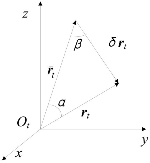
Figure 1.
Geometric interpretation of a pseudorange measurement.
Then, the nominal line of sight and the actual line of sight can be defined in Equations (4) and (5), respectively, as follows:
where and are the subblocks in the block matrix form of and that are defined in Appendix B.
Two angles are defined: observation angle and disturbance angle . Observation angle is the angle between the actual line of sight and the nominal line of sight , and disturbance angle is the angle between the nominal line of sight and position disturbance , that is,
If impulse maneuver is known, position disturbance can be calculated as:
Then, observation angle and disturbance angle can be calculated. Using the sine theorem, under the ideal assumption of no angle measurement noise and no maneuver error, the distance at time can be calculated as:
As shown in Figure 2, it is assumed that the pseudorange measurement error is caused by the angle measurement error and other factors, such as the orbit maneuver error, are not considered. References [20,24] analyzed the relationship between the pseudorange measurement error and the angle measurement error. Assuming that the angle measurement error is , the resulting pseudo distance measurement error can be calculated as:
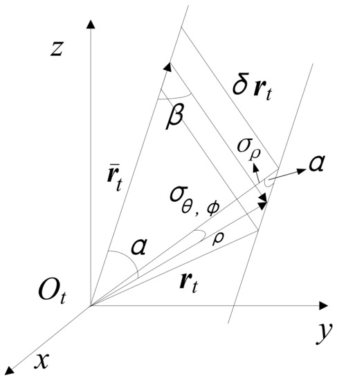
Figure 2.
Pseudorange measurement error caused by the angle measurement error.
In this way, measurement noise matrix of AON based on the orbital maneuver can be obtained as:
2.3. Navigation Accuracy Estimation Based on the FIM and the CRLB
However, for AON, some observability criteria are proposed from the geometric interpretation or linear irrelevant theory, which are essential navigation accuracy criteria. For more extensive-state optimal estimation and filter design analysis, the FIM is a more general tool. The inverse of the FIM is the CRLB, which can be used to calculate the best estimation accuracy that can be obtained in unbiased estimation. Therefore, the CRLB is often used to calculate the best estimation accuracy that can be theoretically achieved. This paper uses the inverse of the FIM, namely, the CRLB, as the estimation criteria of navigation accuracy, which is also a part of the objective function of optimization as discussed in Section 4.
When new observations are obtained at time , the update of the FIM can be described by the following equation:
where represents the FIM at current time , represents the FIM after the new observation is obtained at time , is the state transition matrix from time to time , is the measurement noise with a pseudorange, represents the measurement sensitivity matrix with a pseudorange, and represents the process noise covariance matrix, which is used to describe the unmodeled error of the state transition equation.
The well-known CRLB can be obtained by calculating the inverse matrix of the FIM:
For the traditional angle-only measurement equations, the pseudorange measurement is not included explicitly, and the observation sensitivity matrix of the traditional angle-only measurement equations does not include the pseudorange information. Therefore, the traditional angle-only measurement equations are not directly applicable to the FIM calculation, unless the relative distance has been perfectly determined by the initial orbit determination and the initial state error can be modeled as zero-mean Gaussian white noise. The traditional angle-only observation equation has no observation ability to distinguish distance ambiguity; thus, the estimation of distance of the whole estimation process depends on the initial state with error. When the initial state error is no longer zero-mean Gaussian white noise, such an observation equation and an observation sensitivity matrix can also be calculated by the FIM and the CRLB, which can also converge, but the calculated FIM and CRLB cannot reflect the real estimation accuracy. The CRLB gives the lower bound of the estimation error, but in fact, the estimation error will be much larger than the CRLB, which goes against our original intention of using the CRLB to characterize the accuracy of state estimation. Therefore, this paper introduces the pseudorange measurement to the observation equation, observation sensitivity matrix, and measurement noise matrix to calculate the FIM and the CRLB.
3. Multipulse Glideslope Guidance
A multipulse glideslope approach trajectory is shown in Figure 3. The spacecraft is required to arrive at in a fixed approach time T with a specified velocity from the initial and . Then, a straight line from to denoted by the vector is defined as the approach direction of the multipulse glideslope. At any instant in time, can be expressed as , where and are the magnitude and unit direction of vector , respectively, and can be calculated as:
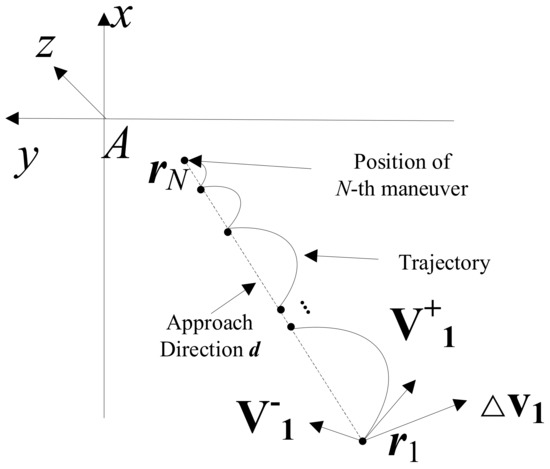
Figure 3.
An example of the multipulse glideslope approach trajectory.
The following linear relationship between and its derivative is adopted to ensure that the approach velocity decreases when the spacecraft approaches the target, shown as following:
where and are constants that can be determined after the boundary conditions for and its derivative at and are substituted as:
The solution to has forms such as:
where , , and are three constants of integration that can be determined after the boundary conditions. Then,
In addition, can be obtained first by numerically solving the following equation:
giving:
Note that if is known, can also be determined.
A total of N pulses are applied during the whole approach process to divide the actual trajectory into segments. Assuming that the time of applying pulses is , where and , the duration of each segment of the trajectory is . After the last pulse is applied, the spacecraft reaches the target point that meets the velocity and position constraints.
Because the approaching trajectory is relatively far from the small body and the gravitational force of a small body is weak, we consider only the gravitational force of the Sun and ignore the gravitational force and other perturbation forces of the small body in the far approach phase. If the initial and terminal position vectors of the spacecraft relative to the asteroid are and , respectively, the i-th maneuver position and time instant of each impulse maneuver in the process of glideslope guidance are written as:
where represents the relative distance of the spacecraft from the terminal position at time instant , which can be calculated using Equation (17).
The relative distance changes exponentially with time. The velocities and , , before and after impulse maneuver at time instant can be expressed as:
where , , and are different blocks in the block form of the state transition matrix defined in Appendix B. According to the initial state and the terminal target state, the following equations can be obtained:
Then, the i-th () maneuver at time instant can be calculated as follows:
5. Numerical Simulation
5.1. Simulation Conditions
Taking 2016HO3 as the object asteroid (see Table 1 for its orbital elements), a simulation study of multipulse glideslope guidance with an enhanced navigation accuracy for the far approach offline was carried out. The start time of the approach rendezvous is shown in Table 2. According to the transfer scheme, it is planned to approach from 100,000 km to 100 km from the asteroid by 6 impulse maneuvers. Table 2 summarizes the simulation parameters used. To verify the effectiveness of the proposed method, different values of the tradeoff weight w between the navigation error objective and the fuel consumption objective were used for Monte Carlo simulation. Each value of the tradeoff weight w was simulated 100 times, and the statistics were analyzed.

Table 1.
Orbit elements of 2016HO3.
Table 2.
Simulation parameters.
5.2. Navigation Accuracy-Enhanced Multipulse Glideslope Guidance Optimum Results
is the tradeoff weight of the fuel consumption objective and the navigation error objective. We conducted a parameter analysis of to show its influence on the resulting optimal maneuvers and the resulting rendezvous trajectory. Different values of the tradeoff weight w were set to solve the optimization problem.
Figure 4 shows the resulting optimal trajectories corresponding to different tradeoff weights w. When w takes a larger value, such as w = 0.5 or 1.0, which means the navigation accuracy is more emphasized, the corresponding trajectories show less deviation from the direction of the approaching straight line after the first maneuver, and the maneuvers are distributed more evenly over relative distances. This result is opposite to the result in [18] in the context of the Vbar approach, because the mission condition in this paper is different with a large initial velocity. At the latter stage of trajectories, all trajectories seem alike, which can be distinguished in the following analysis.

Figure 4.
Resulting optimal trajectories corresponding to different tradeoff weights w.
Figure 5 shows the distributions of the magnitude of s along the optimal trajectories with different w. Overall, the maneuvers show a gradually decreasing trend over time, which verifies the safety benefit of the guidance method. When w takes a larger value, such as 0.5 or 1, the magnitude of the first maneuver is larger, and the magnitude of the second maneuver shows an opposite trend. The small magnitudes of the last two maneuvers with different w are consistent with the relatively small deviation seen at the latter stage of trajectories in Figure 4.
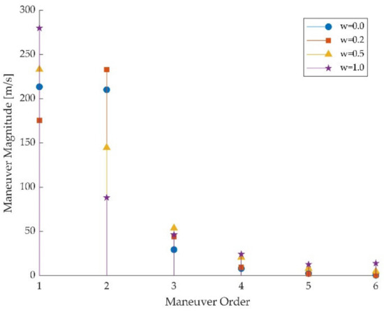
Figure 5.
Distributions of the magnitude of s along the optimal trajectories with different w.
Figure 6 and Figure 7 show how the fuel consumption (total ) and the navigation error objective of the resulting trajectories change with the tradeoff weight w. It is seen that with the increasing w, which means more emphasis is placed on the navigation error objective, the fuel consumption begins to increase and the navigation error objective begins to decrease when w is larger than 0.6, and the navigation error objective starts to play a major role. The tradeoff weight w must be at least 0.7 to bring obvious improvement in navigation accuracy at the cost of extra fuel consumption. A clearer correlation between the fuel consumption and the navigation error objective can be spotted from Figure 8, where these two quantities are plotted. The navigation accuracy continues to improve with the increasing fuel consumption.
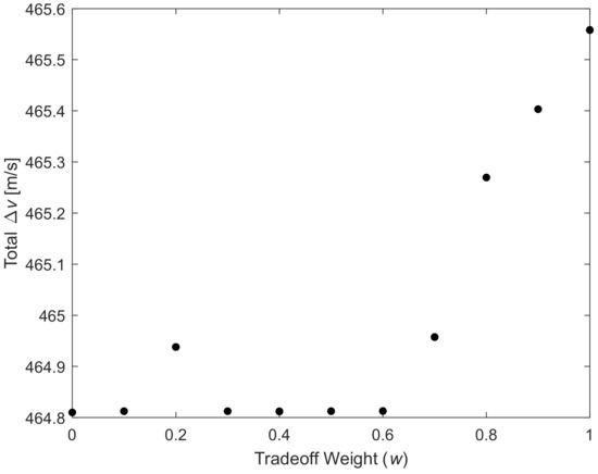
Figure 6.
Fuel consumption vs. tradeoff weight.
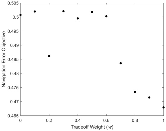
Figure 7.
Navigation error objective vs. tradeoff weight.
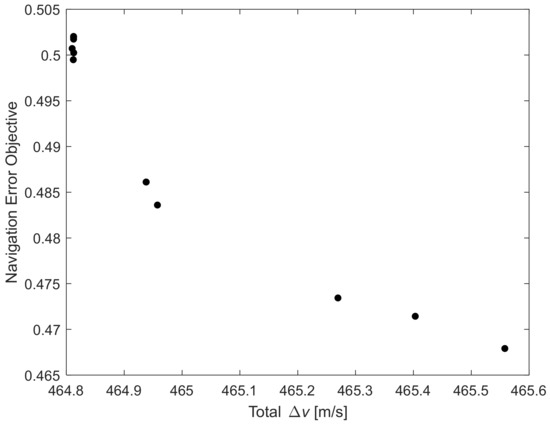
Figure 8.
Navigation error objective vs. fuel cost.
Table 3 shows the distributions of the time instants of s along the optimal trajectories with different w. It can be seen that the distributions are similar, which indicates that the optimal distribution of the time instants of s remains stable and insensitive when w takes different values. However, as shown in Figure 9, the initial relative distance change rate decreases significantly, as w increases. This is attractive, because the optimal distribution of the time instants of s can be solved only once and then fixed when the optimization problem has to be solved multiple times onboard with different w, which will leave initial relative distance change rate as the only optimization variable. Although this will save the time of the optimization computation, it will lead to a satisfactory solution instead of an optimal solution.
Table 3.
Distributions of the time instants of s along the optimal trajectories with different w.
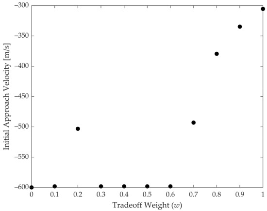
Figure 9.
Initial approaching speed vs. tradeoff weight.
5.3. AON Using Resulting Trajectories
To verify that the proposed guidance strategy can improve the performance of AON, an AON simulation model is constructed, as shown in Figure 10. Navigation filtering [30] is based on the classical Cartesian extended Kalman filter (EKF) and TH equations. The calculated maneuver is directly input into the dynamic model of the spacecraft, regardless of the realization model and the control error of the maneuver.
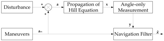
Figure 10.
Simulation model of angle-only navigation using resulting approach maneuvers.
The Monte Carlo simulation for each w includes 100 realizations of truth trajectories and the associated set of angle-only observables generated in each realization. In each realization, the filter model is the EKF, starts with the same nominal reference trajectory and processes the data from the realization. For the case of w = 0.3, the state position errors and the associated uncertainties in each position component and associated RSS (residual sum of squares) are presented in Figure 11. Shown are the 1-sigma and 3-sigma uncertainty bounds as well as the filter solution error obtained by differencing the filter solutions with the truth trajectory. Additionally, listed in the results are statistics of the percentage by which a filter solution exceeds the 1-sigma and the 3-sigma uncertainty bounds. In the present case, the respective percentages are 28.463% and 0.002%, from a population of 13,392,200 samples. Assuming ergodic processes and statistics that conform to a normal distribution, one expects 1-sigma exceedances to be <31.7% of the time and 3-sigma exceedances to be <0.3% of the time, which is true for this case. For the case of w = 0.3, the state velocity errors and the associated uncertainties in each velocity component and the associated RSS (in the lower right) are presented in Figure 12. The statistics of the percentage at which a filter solution exceeds the 1-sigma and 3-sigma bounds show that the filter works normally, which are 28.670% and 0.007%, respectively. Because of the dispersion of initial navigation errors, the dispersion of the navigation errors is still obvious at the early stage of the trajectory, but it then reduces significantly. Another observation with these results is that as the spacecraft is close to the asteroid, the navigation errors fluctuate with the maneuvers, because after each maneuver, it takes some time for the AON filter to converge when the magnitude of the maneuver is relatively small at the latter stage of the trajectory.
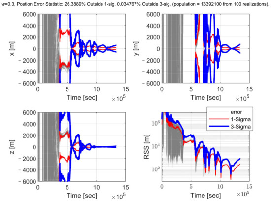
Figure 11.
Angle-only navigation position errors along the resulting trajectory for 100 realizations and uncertainties (1-sigma uncertainty bound in red and 3-sigma uncertainty bound in blue) for the case with w = 0.3.
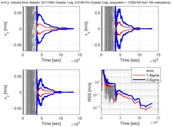
Figure 12.
Angle-only navigation velocity errors along the resulting trajectory for 100 realizations and uncertainties (1-sigma uncertainty bound in red and 3-sigma uncertainty bound in blue) for the case with w = 0.3.
As shown in Figure 13, when the tradeoff weight w increases, the navigation error converges faster first, but the navigation error then increases. In spacecraft rendezvous, there is a quantified minimum navigation accuracy rule, the 1% range rule, which is that the relative navigation accuracy needs to be guaranteed to be at least 1% of the relative distance [23]. Figure 14 shows that along the trajectory, the navigation error converges to less than 1% of the range.
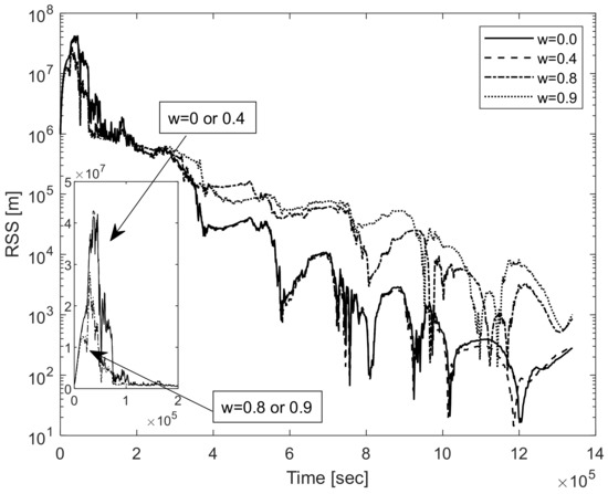
Figure 13.
Sample navigation errors for typical tradeoff weights.
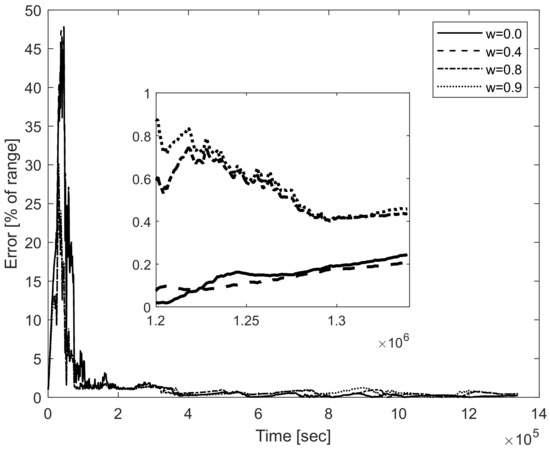
Figure 14.
Sample navigation errors (% of range) for typical tradeoff weights.
As shown in Figure 15, with the increasing tradeoff weight w, the whole navigation error decreases gradually. Tradeoff weight w should be at least 0.7 to see a clear effect. Similarly, Figure 16 shows that the reduction in the whole-range navigation error comes at the cost of increased fuel consumption. As shown in Figure 17 and Figure 18, the arrival navigation error and the whole navigation error show the opposite trend. With the increasing tradeoff weight w and fuel consumption, the arrival navigation error also shows an increasing trend. Therefore, to improve the navigation accuracy at the time of arrival, less fuel can be used; that is, tradeoff weight w can be 0, corresponding to fuel optimal guidance. This shows that the navigation error in the early stage of the approach phase and the navigation error in the later stage or the final arrival navigation error are subject to mutual compromise, which is very important.
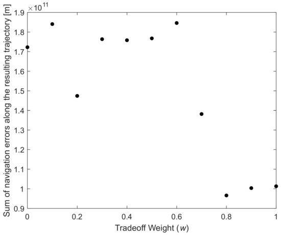
Figure 15.
Sum of navigation errors along the resulting trajectory vs. tradeoff weight w.
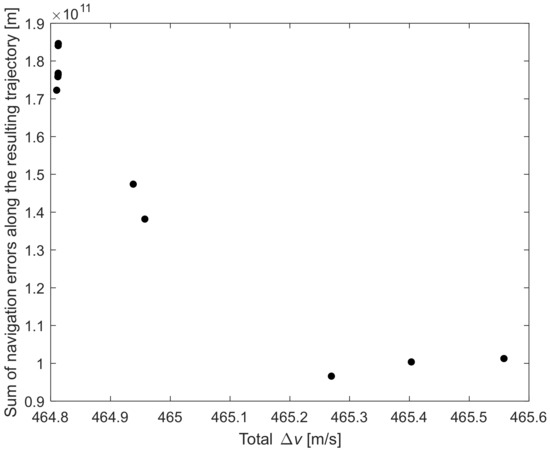
Figure 16.
Sum of navigation errors along the resulting trajectory vs. fuel cost.
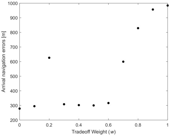
Figure 17.
Arrival navigation error vs. tradeoff weight w.
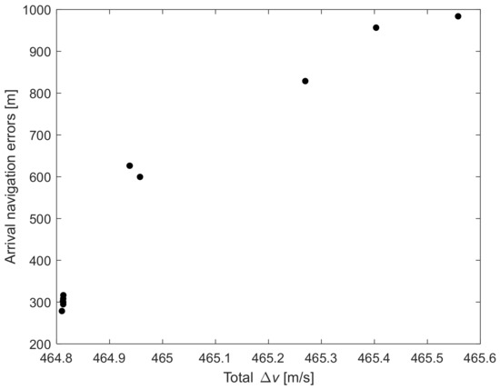
Figure 18.
Arrival navigation error vs. fuel cost.
6. Conclusions
This paper proposes a navigation accuracy-enhanced glideslope guidance method in the context of bearing-only navigation. The tradeoff between the navigation accuracy and the fuel consumption was deeply numerically analyzed. Navigation accuracy can be improved at the cost of extra fuel consumption. The trade-off factor between the navigation accuracy and the fuel consumption has little effect on the pulse maneuver conduction time corresponding to the optimal solution, so the optimal pulse maneuver conduction time can be fixed in engineering implementation. However, the trade-off factor has a very direct impact on the initial relative distance change rate. There is a strong correlation between the navigation accuracy and the fuel consumption trade-off factor, initial relative distance change rate, total fuel consumption, initial maneuver, and navigation accuracy. Therefore, during project implementation, one variable can be changed to change another variable. For example, we can fix the maneuver pulse time and take the change rate of the initial relative distance as the only optimization variable to improve the optimization problem-solving speed. This is attractive for using this method in online closed-loop guidance. The proposed method retains the advantages of a multipulse glideslope guidance method; for example, the approach direction can be designed on demand, and the approach speed decreases with the distance. All these contributions provide a reference for the rendezvous trajectory design of high-precision AON and the design of an autonomous guidance algorithm for the far approach phase of angle-only rendezvous missions.
Author Contributions
Conceptualization, H.Y., D.L. and J.W.; Funding acquisition, J.W.; investigation, H.Y. and J.W.; methodology, H.Y.; validation, H.Y.; writing—original draft, H.Y.; writing—review and editing, D.L. and J.W. All authors have read and agreed to the published version of the manuscript.
Funding
This work is supported by the National Natural Science Foundation of China (No. 11802335) and the National Natural Science Foundation of China (No. 11702321).
Institutional Review Board Statement
Not applicable.
Informed Consent Statement
Not applicable.
Data Availability Statement
Not applicable.
Conflicts of Interest
The authors declare no conflict of interest.
Appendix A. Asteroid Hill Rotation Reference Frame
To describe the relative motion between the spacecraft and the asteroid, the coordinate systems shown in Figure A1 are established, including the asteroid Hill rotation coordinate system and the heliocentric inertial coordinate system . The spacecraft and the asteroid can be regarded as points.
The center is at the barycenter of the asteroid. rotates at the orbital angular velocity relative to . Its basic plane is the asteroid orbital plane, and is defined as follows:
- The axis is inward along the orbit radius;
- The axis follows the angular momentum direction of the asteroid’s orbit;
- The axis completes the right-handed coordinate system and is perpendicular to the axis in the orbital plane.
The unit vector corresponding to the asteroid Hill rotation coordinate system is , and the unit vector corresponding to the heliocentric inertial coordinate system is .
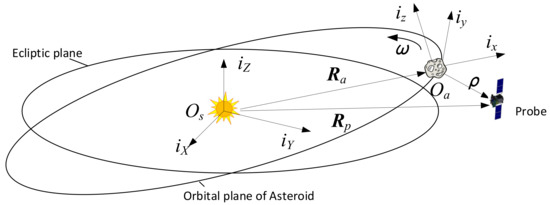
Figure A1.
Definition of asteroid Hill rotation coordinate systems.
Appendix B. Tschauner–Hempel Equation of a Relative Motion
The relative motion between the spacecraft and the asteroid is shown in Figure A1. If the asteroid travels in an elliptical orbit around the Sun, the asteroid orbit in the heliocentric inertial system can be described by classical orbit elements, that is, the semimajor axis, eccentricity, inclination, longitude of the ascending node, perihelion argument angle, and true anomaly .
Therefore, the state transition matrix can be defined as:
For the specific details of , see [28]. The state transition matrix is transferred from the true anomaly frame to the time frame; then,
If , then , , , and can be abbreviated as , , , and , respectively. Then, Φ (t) can be described as:
The input matrix corresponding to the impulse maneuver at time is ; then,
If is a sampling step, then,
Appendix C. Angle Measurement and Pseudodistance Measurement
The angle-only measurement equation based on the orbital maneuver includes the real measurement of the azimuth angle and the elevation angle of the spacecraft relative to the target asteroid and the pseudo measurement of distance of the spacecraft relative to the target. These angles and distances are defined in the asteroid Hill rotation coordinate system, as shown in Figure A2. The azimuth angle is defined from 0° to 180°, and the elevation angle is set to be from –90° to +90°.
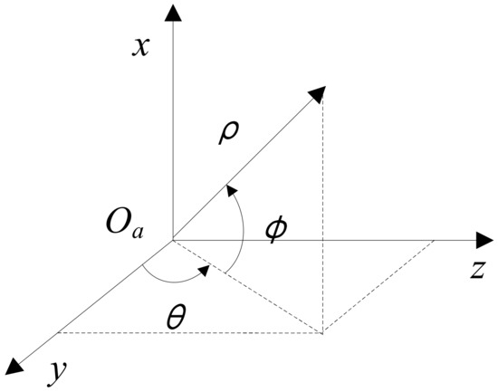
Figure A2.
Measurement angle and relative distance of the asteroid in the asteroid Hill rotating reference frame.
References
- Rivkin, A.S.; Chabot, N.L.; Stickle, A.M.; Thomas, C.A.; Richardson, D.C.; Barnouin, O.; Fahnestock, E.G.; Ernst, C.M.; Cheng, A.F.; Chesley, S.; et al. The Double Asteroid Redirection Test (DART): Planetary Defense Investigations and Requirements. Planet. Sci. J. 2021, 2, 173. [Google Scholar] [CrossRef]
- Vaughan, R.; Riedel, J.; Davis, R.; Owen, J.W.; Synnott, S. Optical navigation for the Galileo Gaspra encounter. In Proceedings of the Astrodynamics Conference, Hilton Head Island, SC, USA, 10–12 August 1992; p. 4522. [Google Scholar]
- Miller, J.K.; Williams, B.G.; Bollman, W.E.; Davis, R.P.; Yeomans, D.K. Navigation analysis for Eros rendezvous and orbital phases. J. Astronaut. Sci. 1995, 43, 453–476. [Google Scholar]
- Broschart, S.; Bhaskaran, S.; Bellerose, J.; Dietrich, A.; Han, D.; Haw, R.; Mastrodemos, N.; Owen, W.M.; Rush, B.; Surovik, D. Shadow navigation support at jpl for the rosetta landing on comet 67p/churyumov-gerasimenko. In Proceedings of the 26th International Symposium on Space Flight Dynamics ISSFD, number ISSFD-2017-096, Matsuyama, Japan, 3–9 June 2017. [Google Scholar]
- Kominato, T.; Matsuoka, M.; Uo, M.; Hashimoto, T.; Kawaguchi, J.I. Optical hybrid navigation and station keeping around Itokawa. In Proceedings of the AIAA/AAS Astrodynamics Specialist Conference and Exhibit, Keystone, Colorado, 21–24 August 2006; p. 6535. [Google Scholar]
- Tsuda, Y.; Takeuchi, H.; Ogawa, N.; Ono, G.; Kikuchi, S.; Oki, Y.; Ishiguro, M.; Kuroda, D.; Urakawa, S.; Okumura, S.-I. Rendezvous to asteroid with highly uncertain ephemeris: Hayabusa2’s Ryugu-approach operation result. Astrodynamics 2020, 4, 137–147. [Google Scholar] [CrossRef]
- Lamey, Q.; Vance, L.D.; Thangavelautham, J. The Impact of the Yarkosvky Effect on Satellite Navigation around Small Bodies. ASCEND 2021 2021, 2021, 4173. [Google Scholar]
- Yu, Z.; Shang, H.; Wei, B. Accessibility assessment and trajectory design for multiple Near-Earth-asteroids exploration using stand-alone CubeSats. Aerosp. Sci. Technol. 2021, 118, 106944. [Google Scholar] [CrossRef]
- Gil-Fernandez, J.; Prieto-Llanos, T.; Cadenas-Gorgojo, R.; Graziano, M.; Drai, R. Autonomous GNC Algorithms for Rendezvous Missions to Near-Earth-Objects. In Proceedings of the AIAA/AAS Astrodynamics Specialist Conference & Exhibit, Honolulu, HI, USA, 18–21 August 2008. [Google Scholar]
- Bhaskaran, S. Autonomous navigation for deep space missions. SpaceOps 2012 2012, 2012, 1267135. [Google Scholar]
- Vetrisano, M.; Yarnoz, D.G.; Branco, J. Effective approach navigation prior to small body deflection. In Proceedings of the Space Generation Congress, Beijing, China, 23–27 September 2013. [Google Scholar]
- Richards, A.; Feron, E.; How, J.P.; Schouwenaars, T. Spacecraft Trajectory Planning with Avoidance Constraints Using Mixed-Integer Linear Programming. J. Guid. Control. Dyn. 2002, 25, 755–764. [Google Scholar] [CrossRef] [Green Version]
- Boyd, S.; Vandenberghe, L. Convex Optimization; Cambridge University Press: Cambridge, UK, 2004. [Google Scholar]
- Weiss, A.; Baldwin, M.; Erwin, R.S.; Kolmanovsky, I. Model Predictive Control for Spacecraft Rendezvous and Docking: Strategies for Handling Constraints and Case Studies. IEEE Trans. Control. Syst. Technol. 2015, 23, 1638–1647. [Google Scholar] [CrossRef]
- Hartley, E. A tutorial on model predictive control for spacecraft rendezvous. In Proceedings of the Control Conference, Osaka, Japan, 15–18 December 2015. [Google Scholar]
- Hablani, H.B.; Tapper, M.L.; Dana-Bashian, D.J. Guidance and Relative Navigation for Autonomous Rendezvous in a Circular Orbit. J. Guid. Control. Dyn. 2002, 25, 553–562. [Google Scholar] [CrossRef]
- Benedikter, B.; Zavoli, A. Convex Optimization of Linear Impulsive Rendezvous. arXiv 2019, arXiv:1912.08038. [Google Scholar]
- Grzymisch, J.; Fichter, W. Optimal Rendezvous Guidance with Enhanced Bearings-Only Observability. J. Guid. Control. Dyn. 2015, 38, 1131–1140. [Google Scholar] [CrossRef]
- Woffinden, D.C.; Geller, D.K. Observability Criteria for Angles-Only Navigation. IEEE Trans. Aerosp. Electron. Syst. 2009, 45, 1194–1208. [Google Scholar] [CrossRef]
- Woffinden, D.C.; Geller, D.K. Optimal Orbital Rendezvous Maneuvering for Angles-Only Navigation. J. Guid. Control Dyn. 2009, 32, 1382–1387. [Google Scholar] [CrossRef]
- Grzymisch, J.; Fichter, W. Observability Criteria and Unobservable Maneuvers for In-Orbit Bearings-Only Navigation. J. Guid. Control Dyn. 2014, 37, 1250–1259. [Google Scholar] [CrossRef]
- Grzymisch, J.; Fichter, W. Analytic Optimal Observability Maneuvers for In-Orbit Bearings-Only Rendezvous. J. Guid. Control Dyn. 2014, 37, 1658–1664. [Google Scholar] [CrossRef]
- Mok, S.-H.; Pi, J.; Bang, H. One-step rendezvous guidance for improving observability in bearings-only navigation. Adv. Space Res. 2020, 66, 2689–2702. [Google Scholar] [CrossRef]
- Hou, B.; Wang, D.; Wang, J.; Ge, D.; Zhou, H.; Zhou, X. Optimal Maneuvering for Autonomous Relative Navigation Using Monocular Camera Sequential Images. J. Guid. Control Dyn. 2021, 44, 1947–1960. [Google Scholar] [CrossRef]
- D’Amico, S.; Ardaens, J.S.; Gaias, G.; Benninghoff, H.; Schlepp, B.; Jorgensen, J.L. Noncooperative Rendezvous Using Angles-Only Optical Navigation: System Design and Flight Results. J. Guid. Control Dyn. 2013, 36, 1576–1595. [Google Scholar] [CrossRef]
- Pesce, V.; Opromolla, R.; Sarno, S.; Lavagna, M.; Grassi, M. Autonomous relative navigation around uncooperative spacecraft based on a single camera. Aerosp. Sci. Technol. 2019, 84, 1070–1080. [Google Scholar] [CrossRef]
- Clohessy, W.H.; Wiltshire, R.S. Terminal Guidance System for Satellite Rendezvous. J. Aerosp. Sci. 1960, 27, 653–658. [Google Scholar] [CrossRef]
- Okasha, M.; Newman, B. Guidance, Navigation and Control for Satellite Proximity Operations using Tschauner-Hempel Equations. J. Astronaut. Sci. 2013, 60, 109–136. [Google Scholar] [CrossRef]
- Yamanaka, K.; Ankersen, F. New State Transition Matrix for Relative Motion on an Arbitrary Elliptical Orbit. J. Guid. Control Dyn. 2002, 25, 60–66. [Google Scholar] [CrossRef]
- Arthur, G. Applied Optimal Estimation; The MIT Press: Cambreidge, MA, USA, 1974. [Google Scholar]
Publisher’s Note: MDPI stays neutral with regard to jurisdictional claims in published maps and institutional affiliations. |
© 2022 by the authors. Licensee MDPI, Basel, Switzerland. This article is an open access article distributed under the terms and conditions of the Creative Commons Attribution (CC BY) license (https://creativecommons.org/licenses/by/4.0/).