
Clean Sky 2 Technology Evaluator—Results of the First Air Transport System Level Assessments

Abstract
:1. Introduction
2. Model Overview
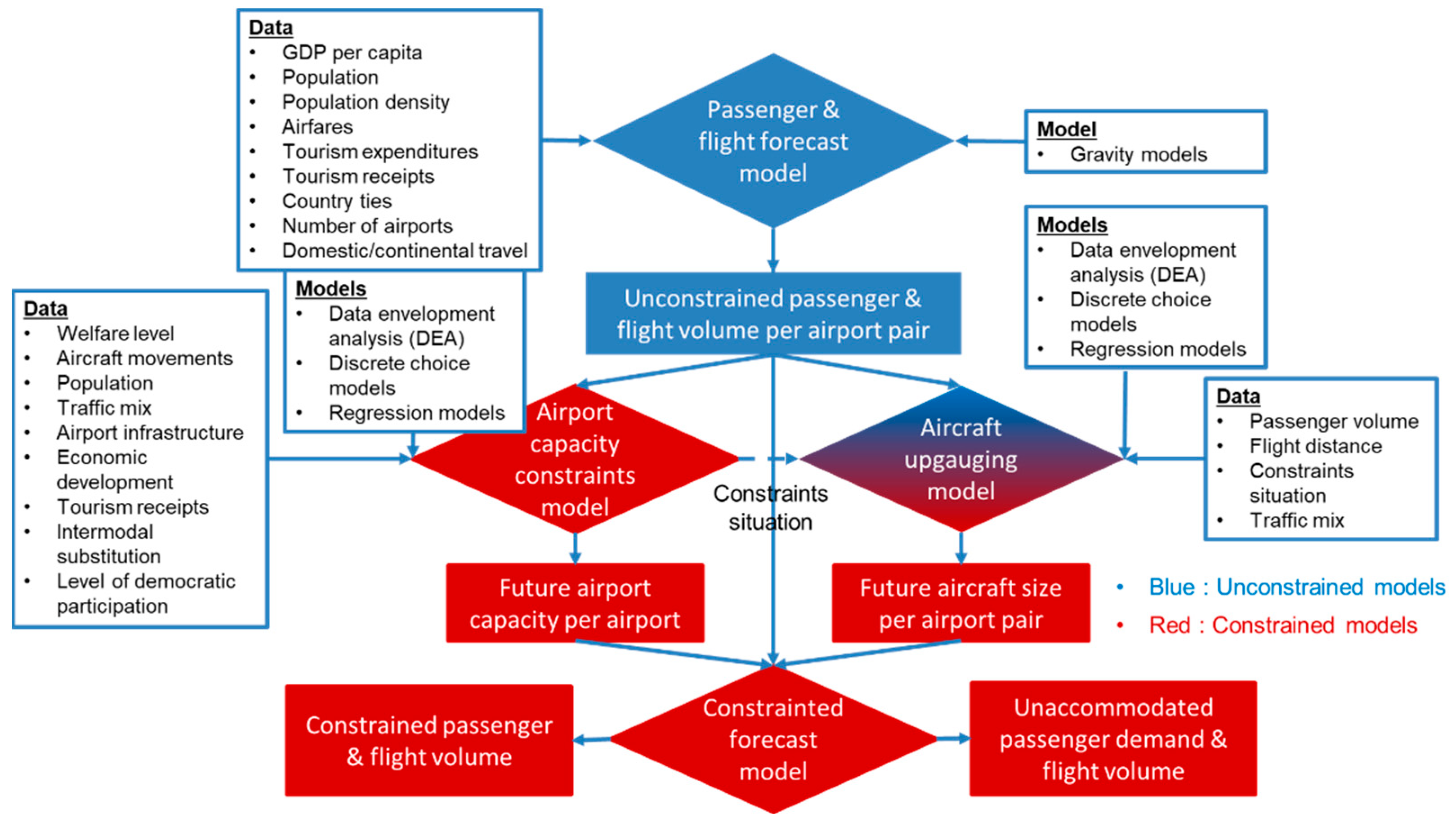
2.1. Passenger and Flight Forecasts
- In the first step, unconstrained passenger demand and flight volume is forecast for each airport pair.
- In the next step, for each airport pair, the flight volume is compared with the current and expected airport capacity. The forecast passenger and flight volume, as well as the constraint situation at airports, will influence the average future aircraft size, which is forecast for each airport pair.
- In the final step, the expected passenger and flight volume is balanced with airport capacity and aircraft size development to yield the constrained passenger and flight volume. This might result in some unaccommodated passenger demand and flight volume, depending on the severity of airport capacity constraints and the potential of employing larger aircraft.
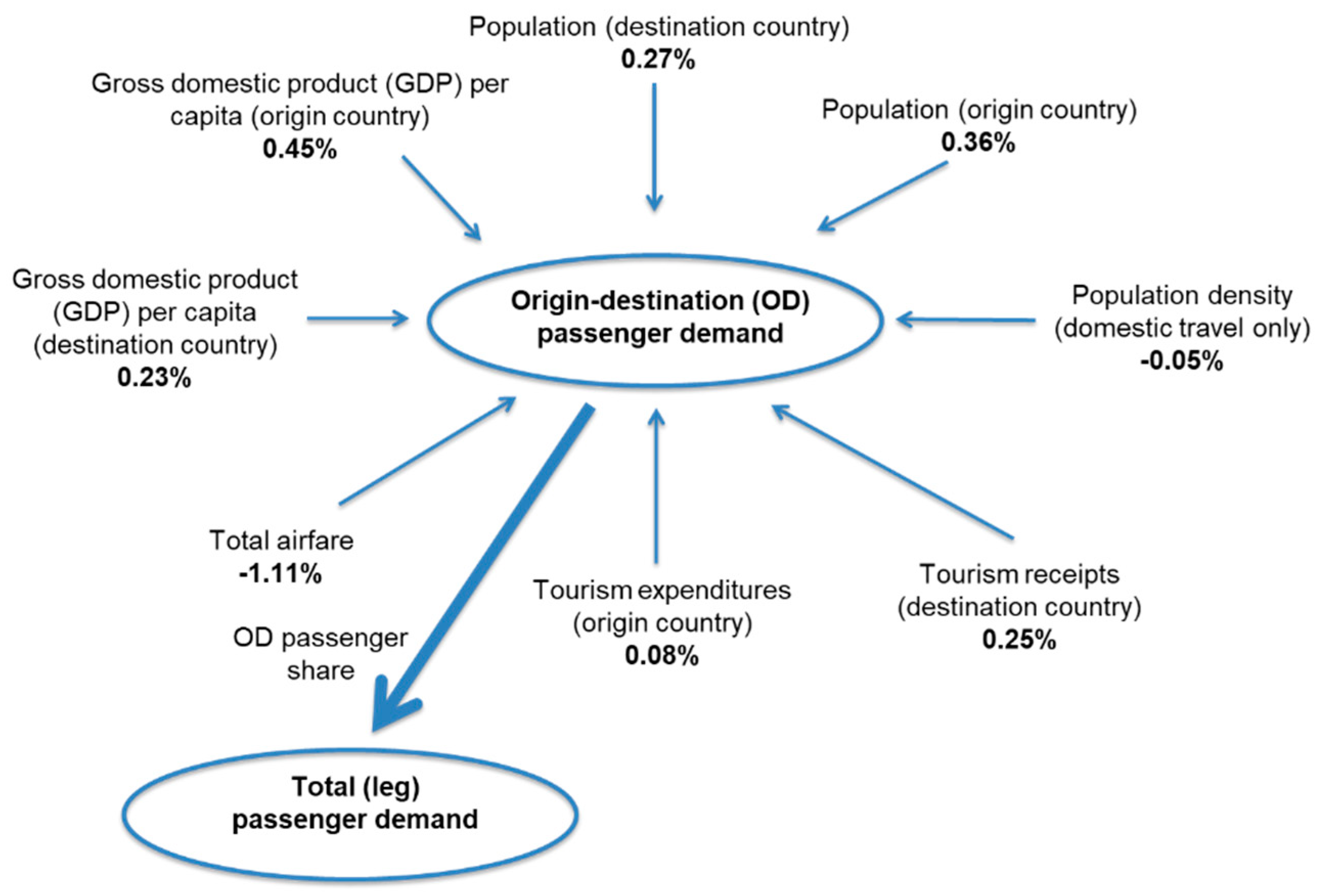
- Air passenger demand, which is origin–destination (OD) passenger flows, and the total passenger flows including transfer passengers, between countries as well as airports.
- Airport capacity and capacity utilisation.
- Airport capacity enlargements and limits.
- Average aircraft size: the average number of passengers per flight.
2.1.1. Air Passenger Demand
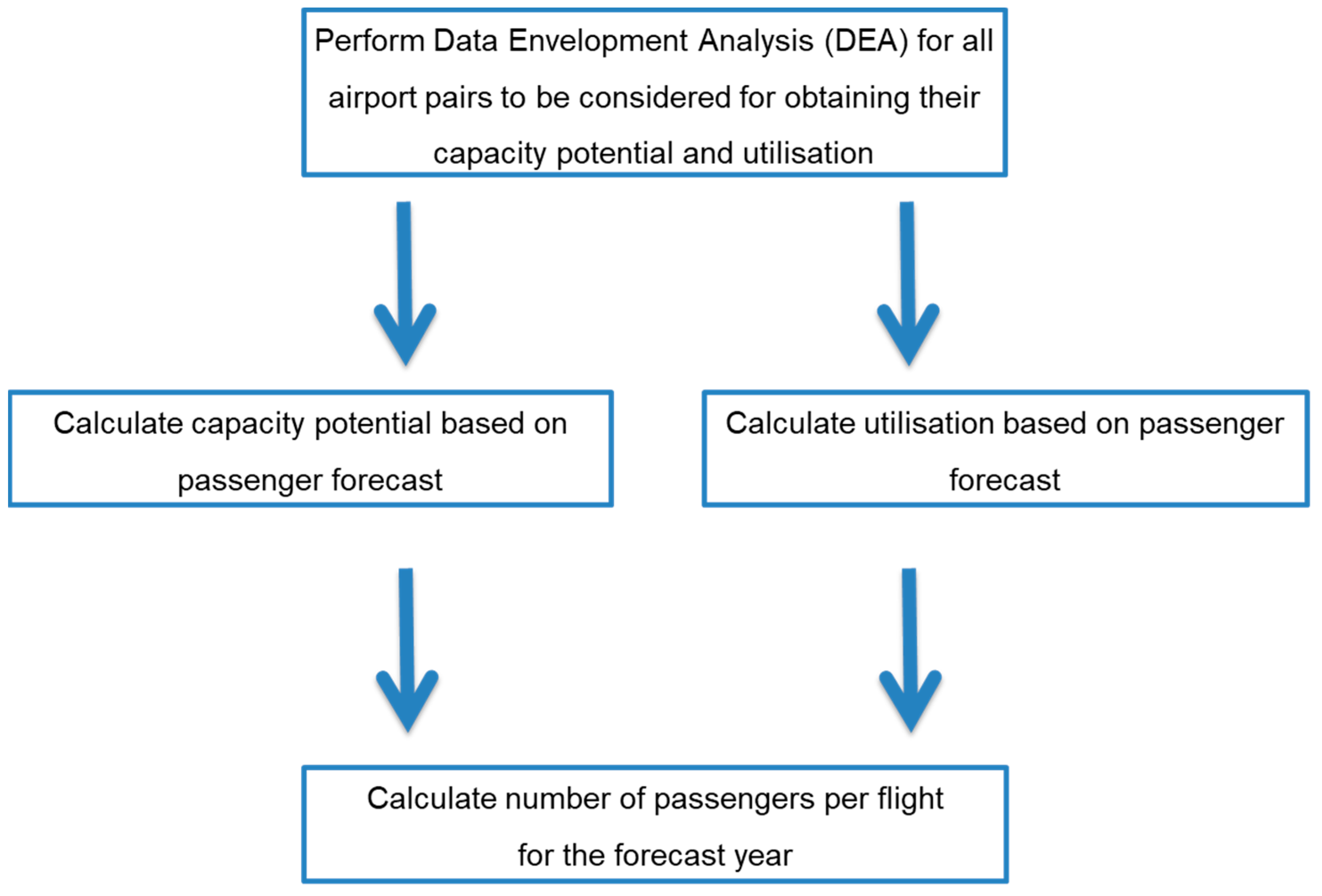
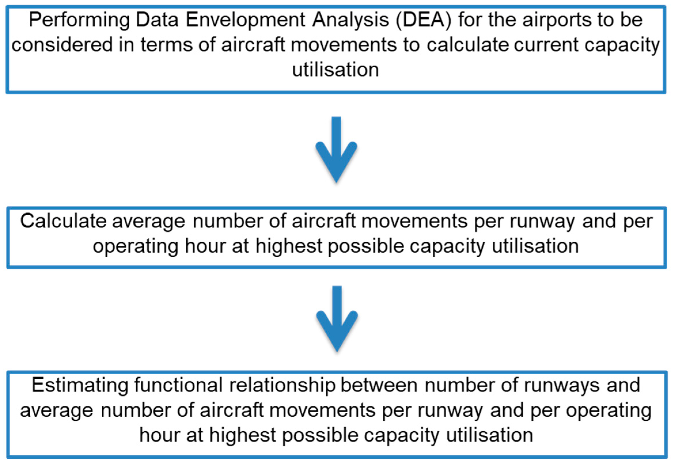
2.1.2. Airport Capacity and Capacity Utilisation
- The first step is the use of the aforementioned DEA to estimate the current airport capacity for airports of interest.
- In a second step, the average number of aircraft movements per runway and per operating hour at the highest possible level of capacity utilisation for each airport is calculated.
- The last step is to perform a regression analysis based on the results of the DEA.
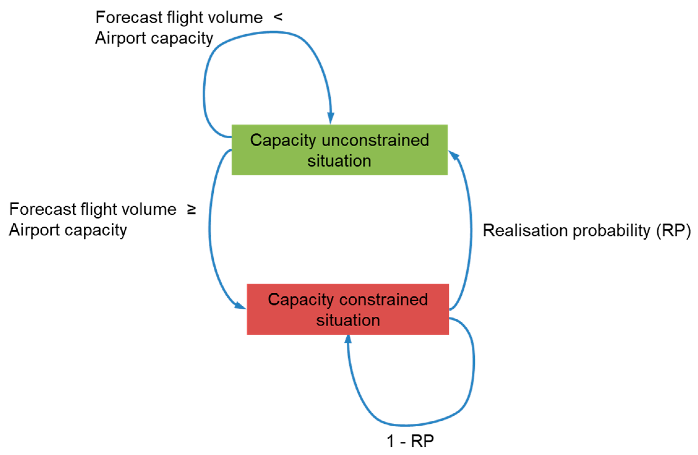
2.1.3. Airport Capacity Enlargements and Limits
- Situation one: forecast demand < airport capacity.
- Situation two: forecast demand ≥ airport capacity.
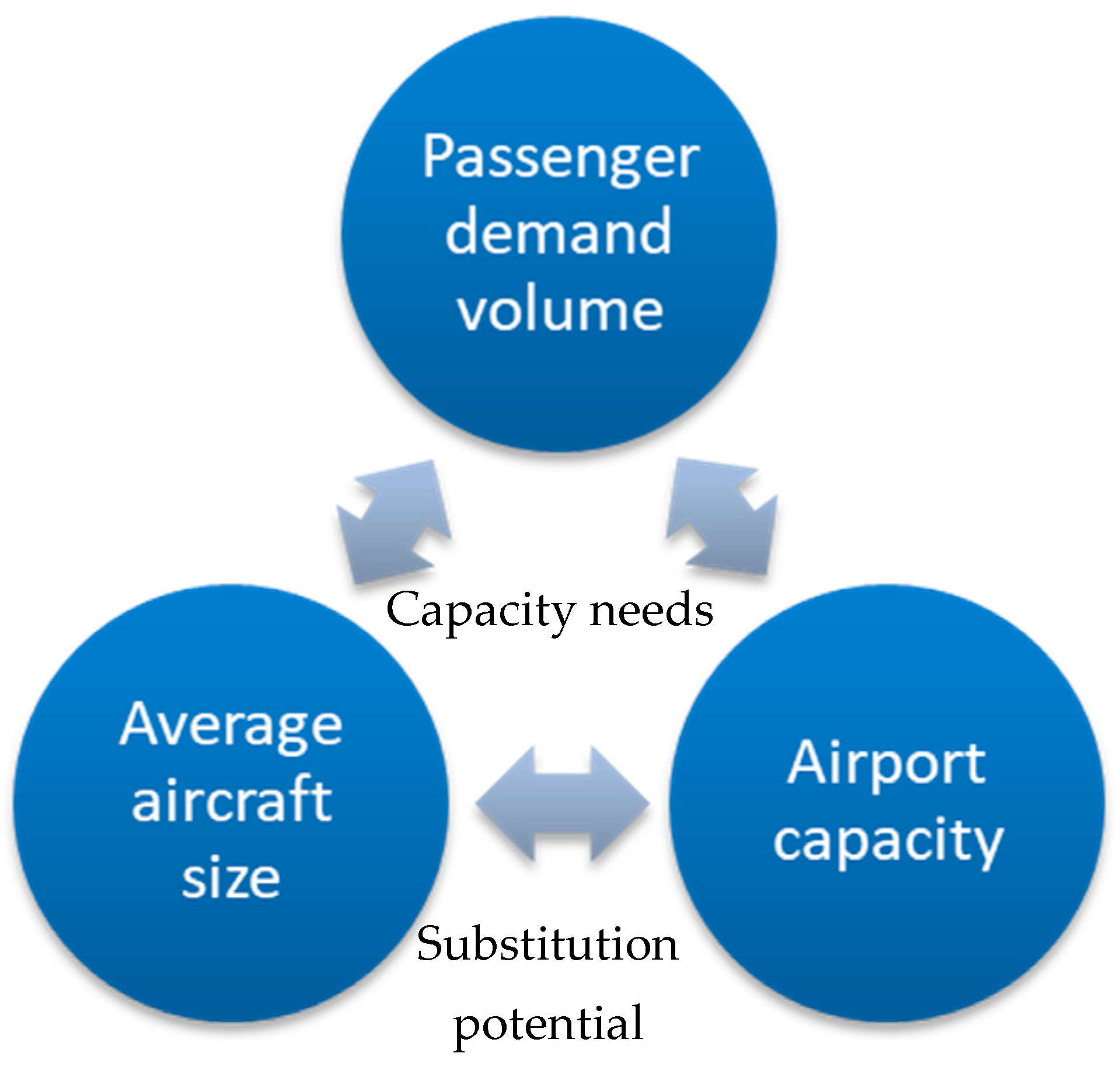
2.1.4. Average Aircraft Size: Average Number of Passengers per Flight
2.2. Aircraft Fleet Forecast
- The passenger traffic forecast, including the future number of passengers and flights per airport pair (Section 2.1).
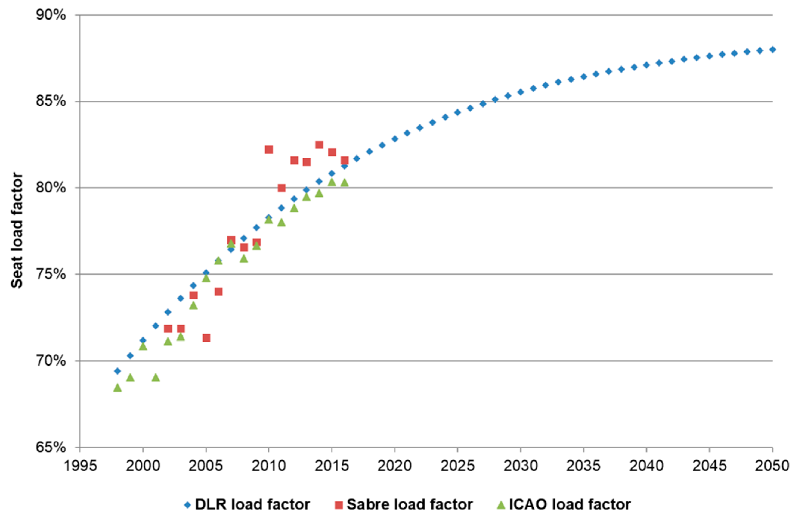
- The seat load factor forecast for the conversion of the passengers per flight to the seats offered per flight.
- The base year, i.e., 2014 flight schedules as a list of flight operations by airport pair and aircraft type.
- The base-year fleet data.
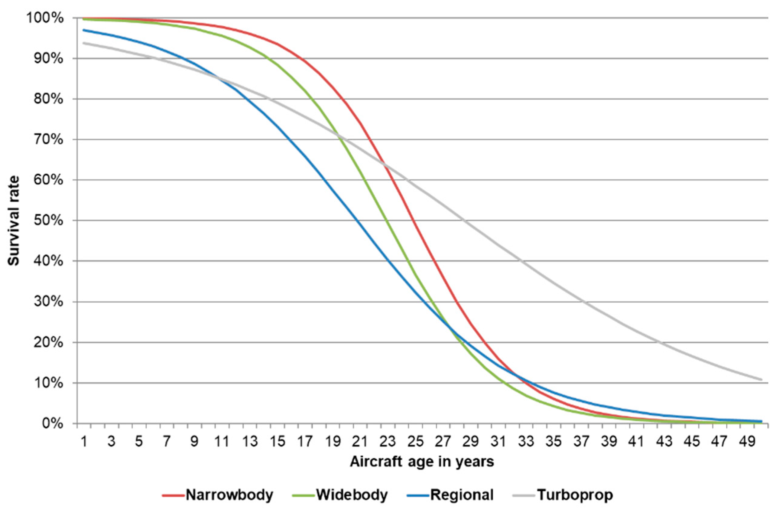
- Aircraft retirement curves.
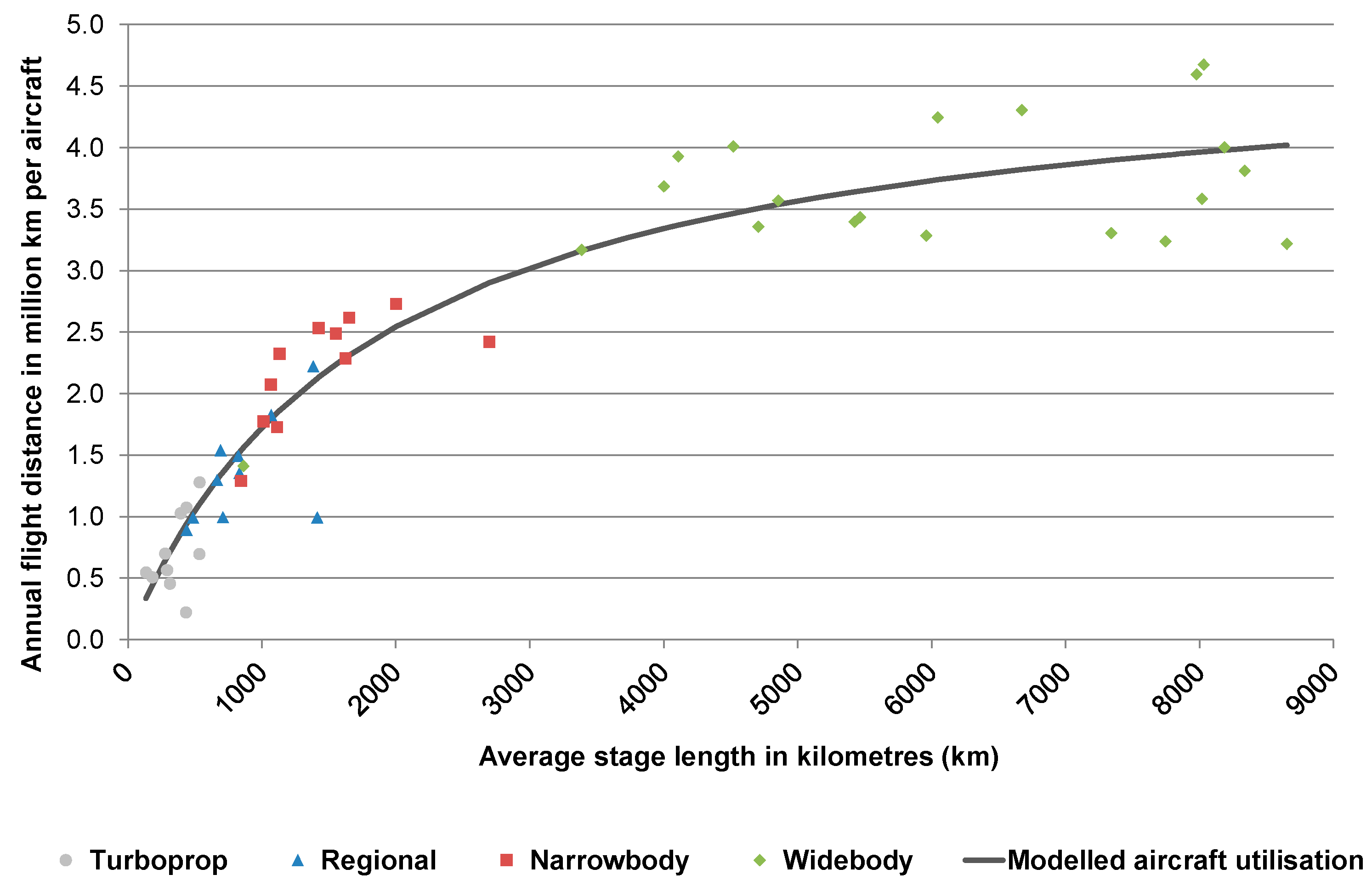
- Aircraft utilisation assumptions.
- A list of available aircraft (production window = the time between entry into service and the out-of-production date of an aircraft type) in each seat category.
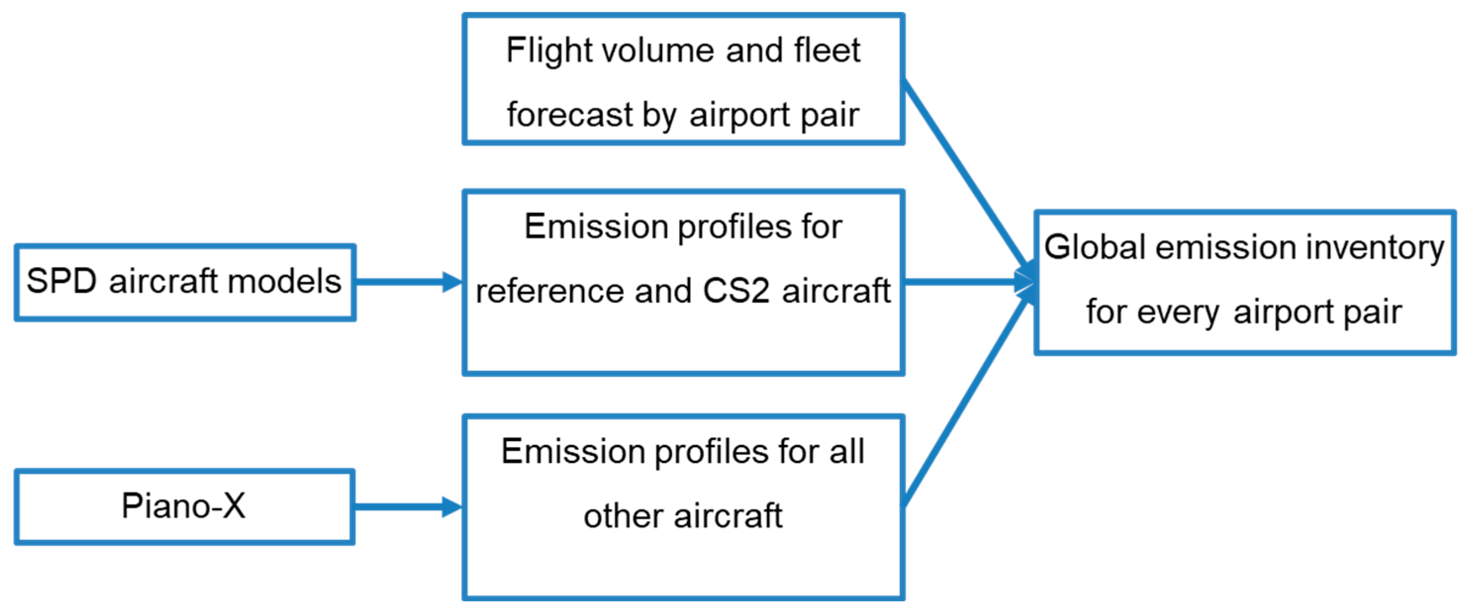
2.3. Emission Modelling
3. Results
- the passenger demand and flight volume (Section 3.1).
- the aircraft fleet (Section 3.2).
- the aircraft emissions (Section 3.3).
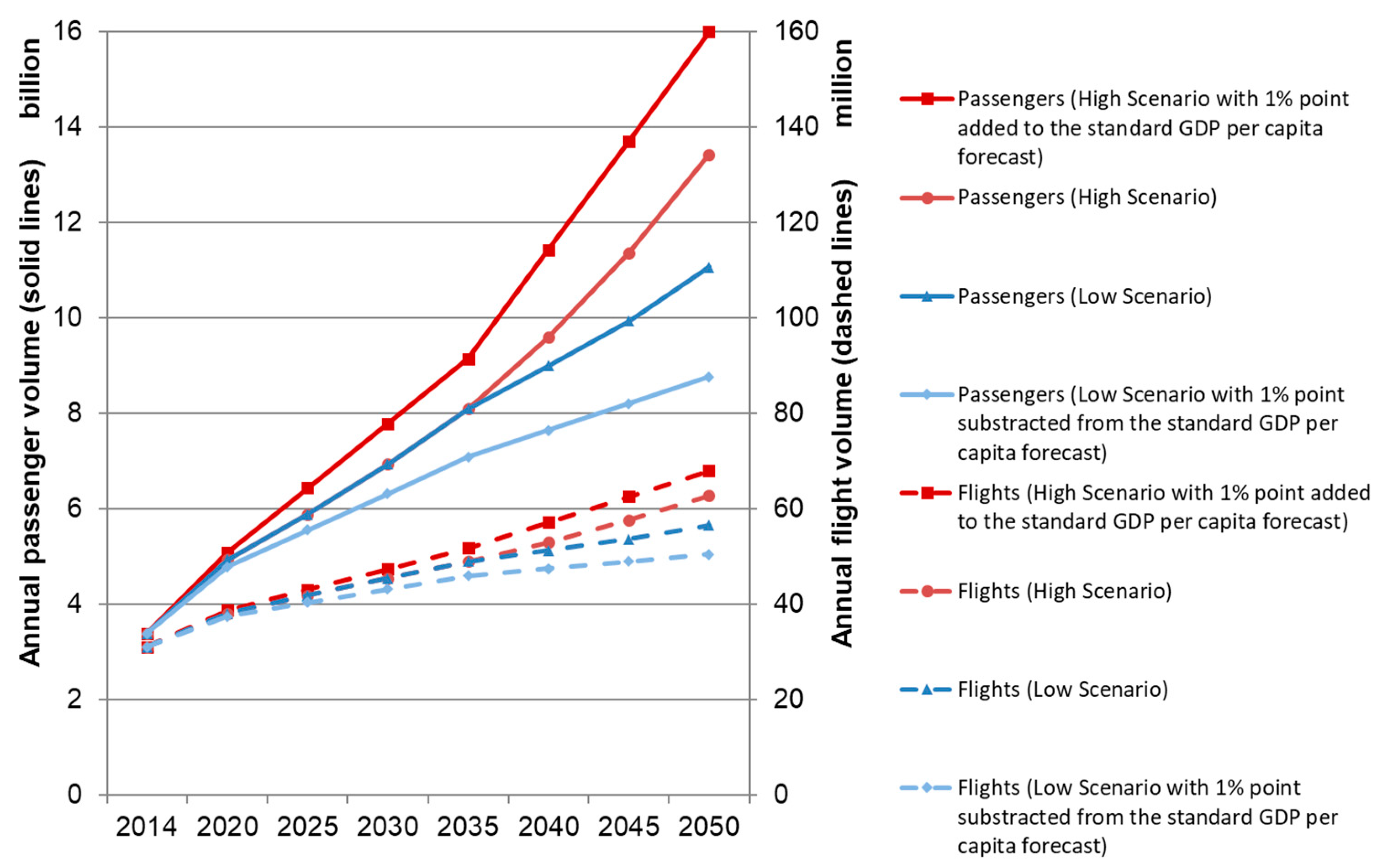
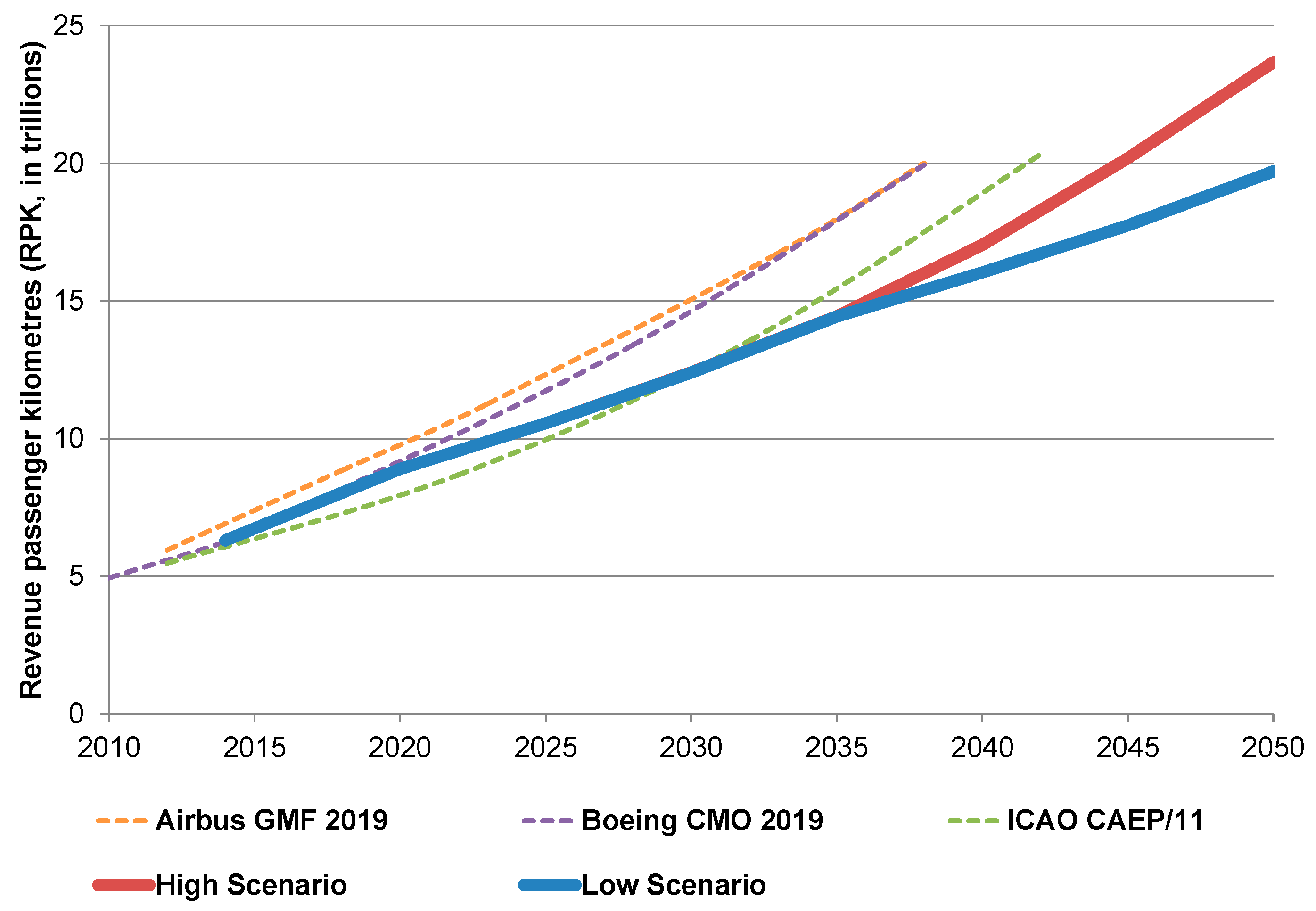
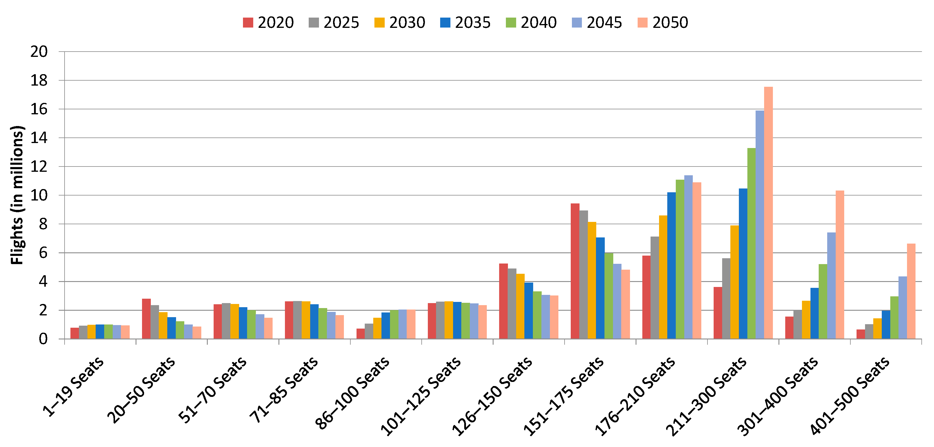
3.1. Passenger Demand and Flight Volume
- we can increase the number of passengers per flight (and hold the numbers of flights constant),
- we can increase the number of flights (and hold the passengers per flight transported constant),
- we can mix both options.
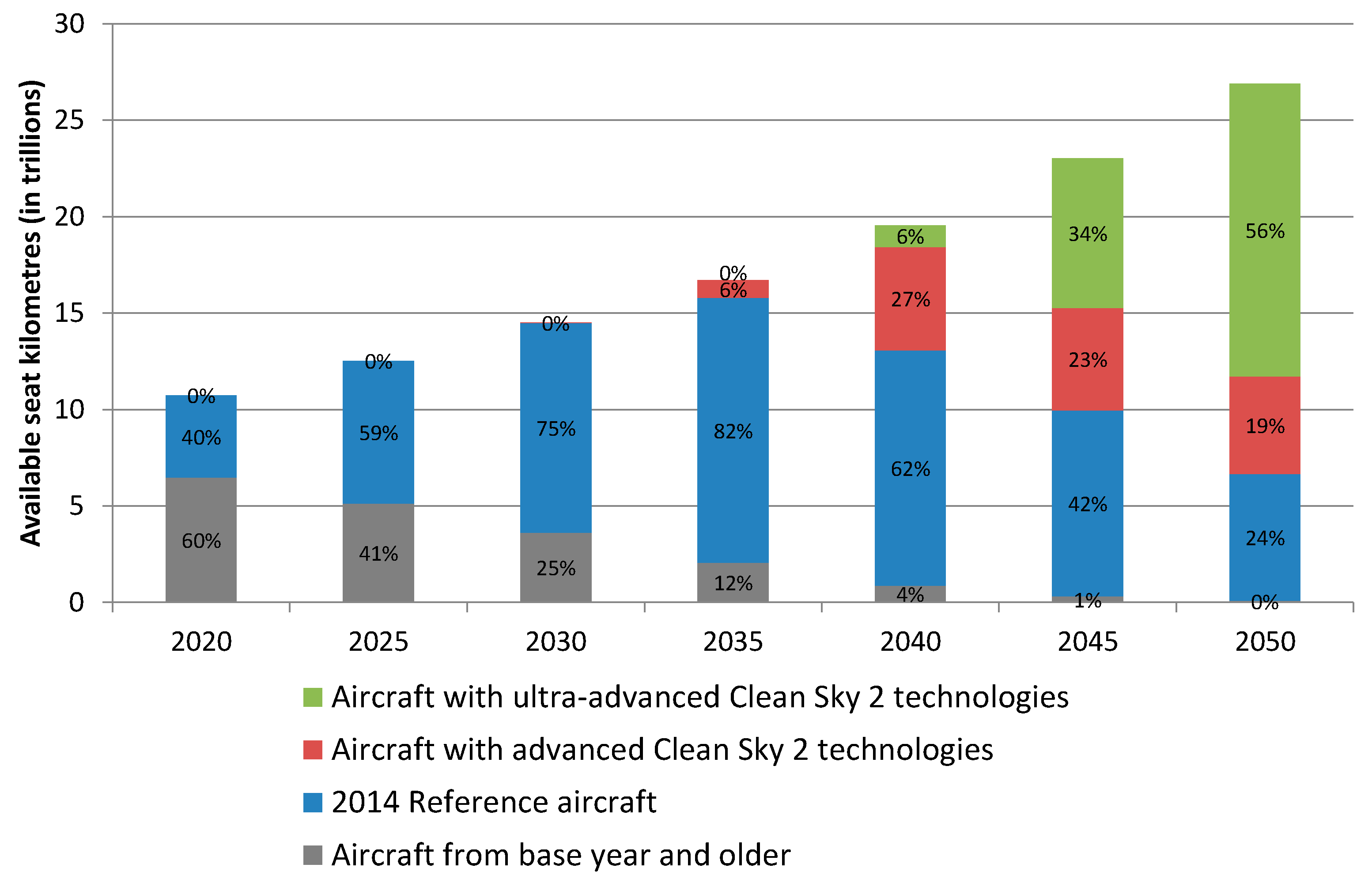
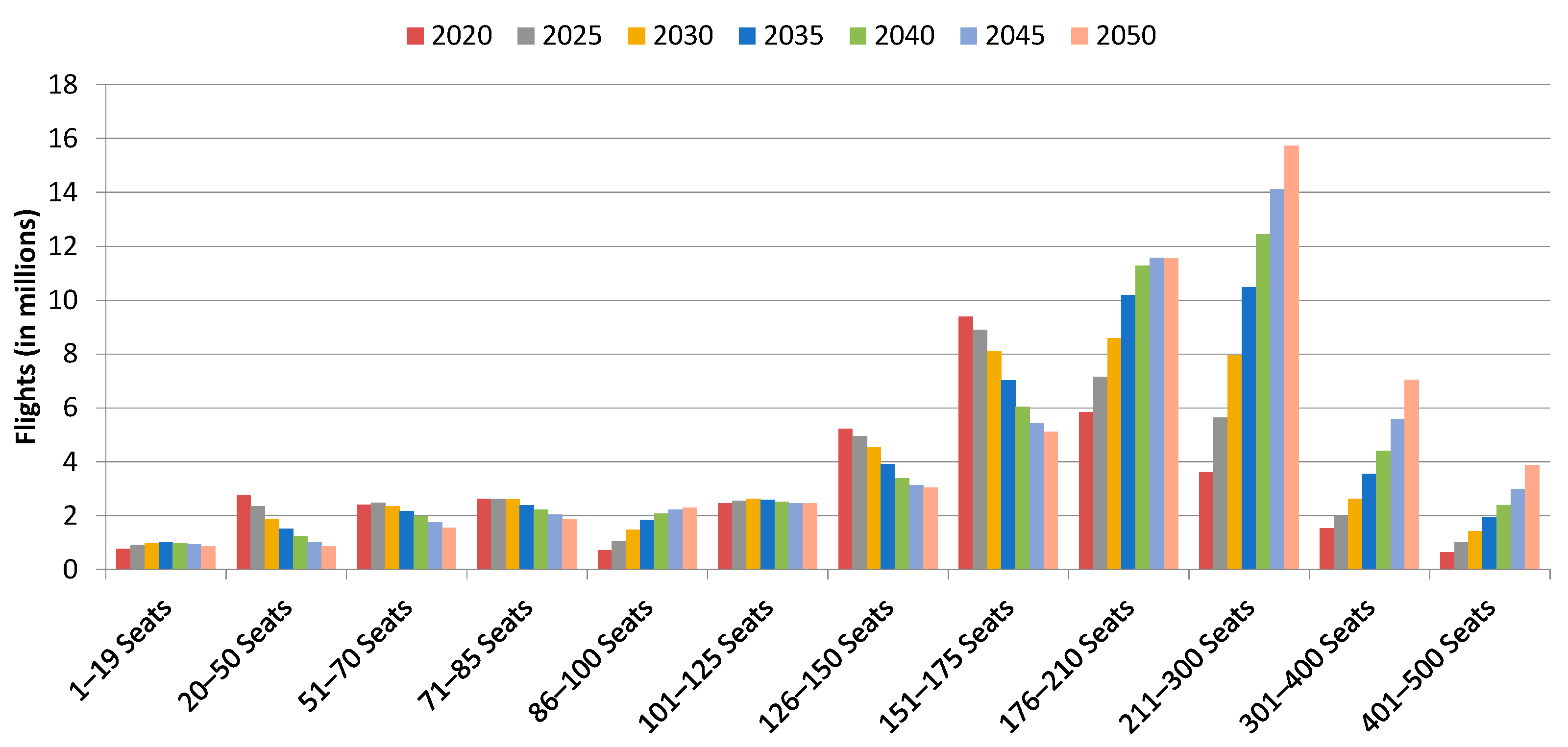
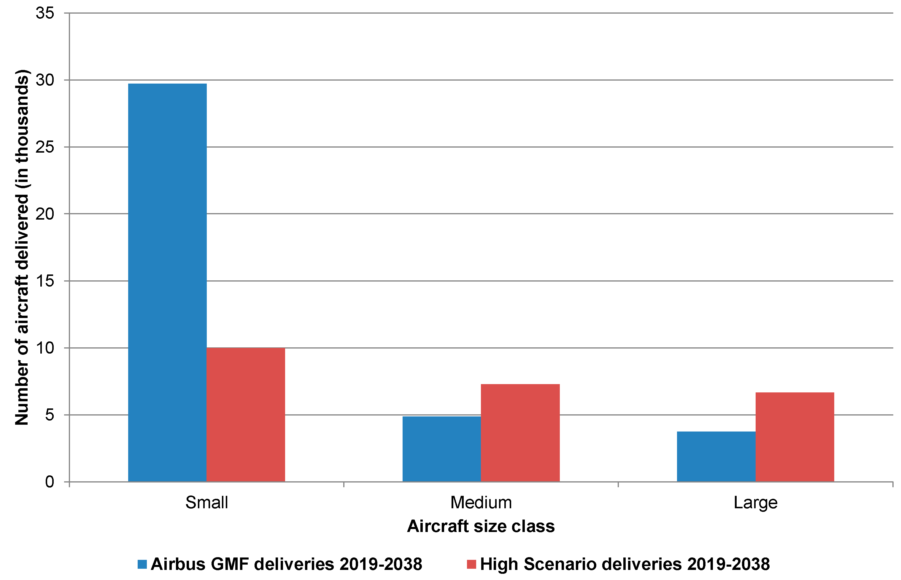
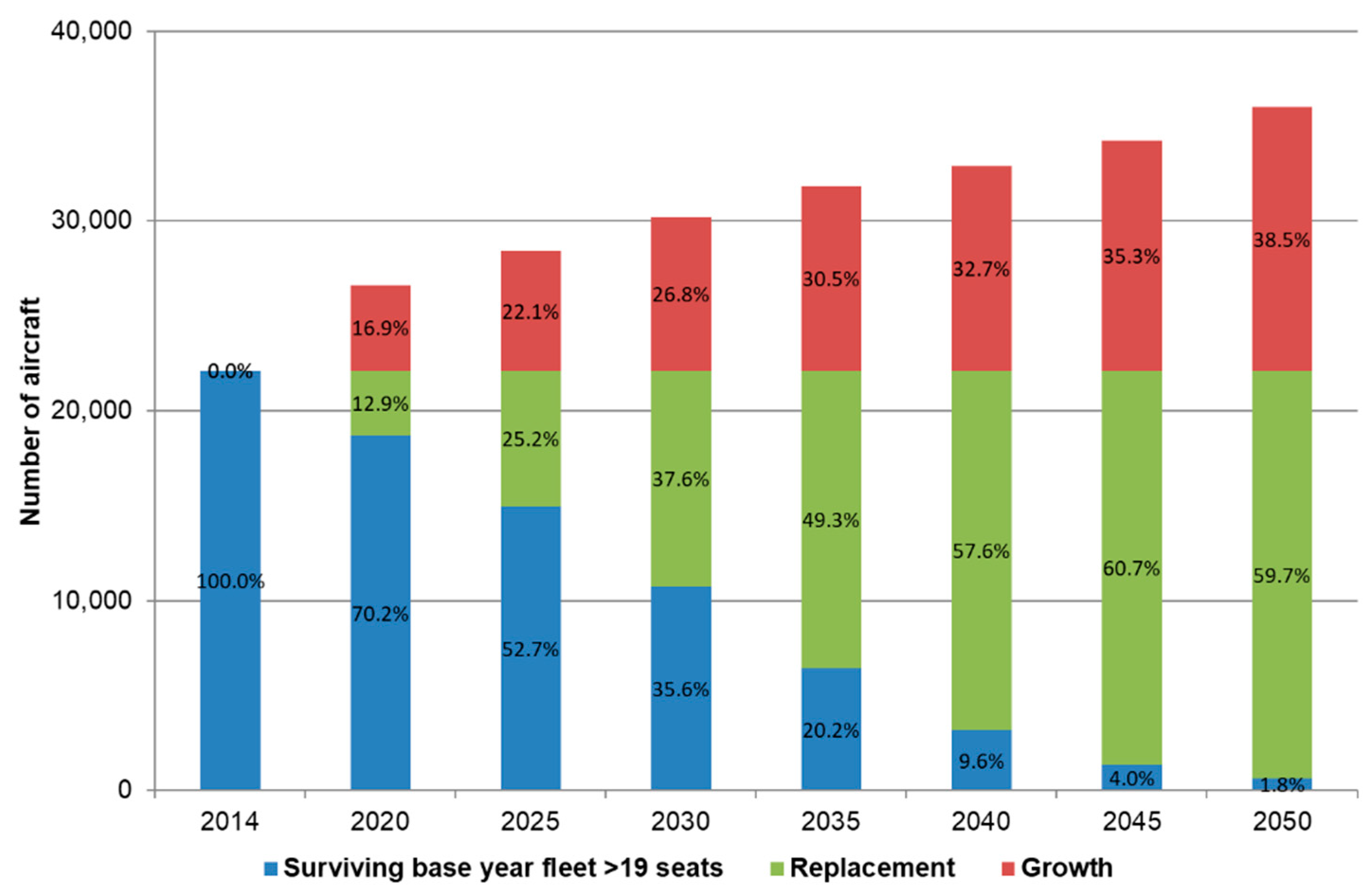
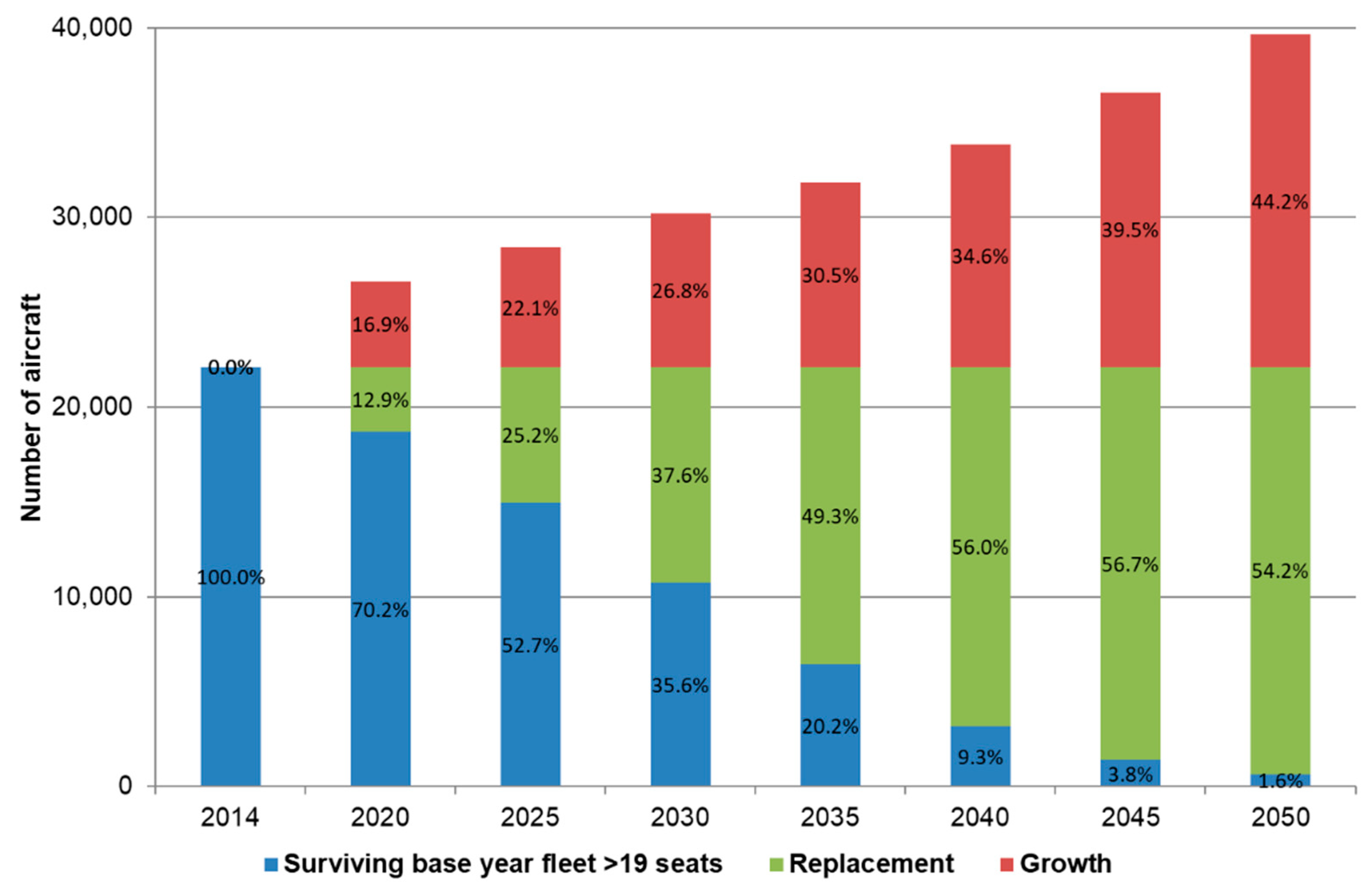
3.2. Aircraft Fleet
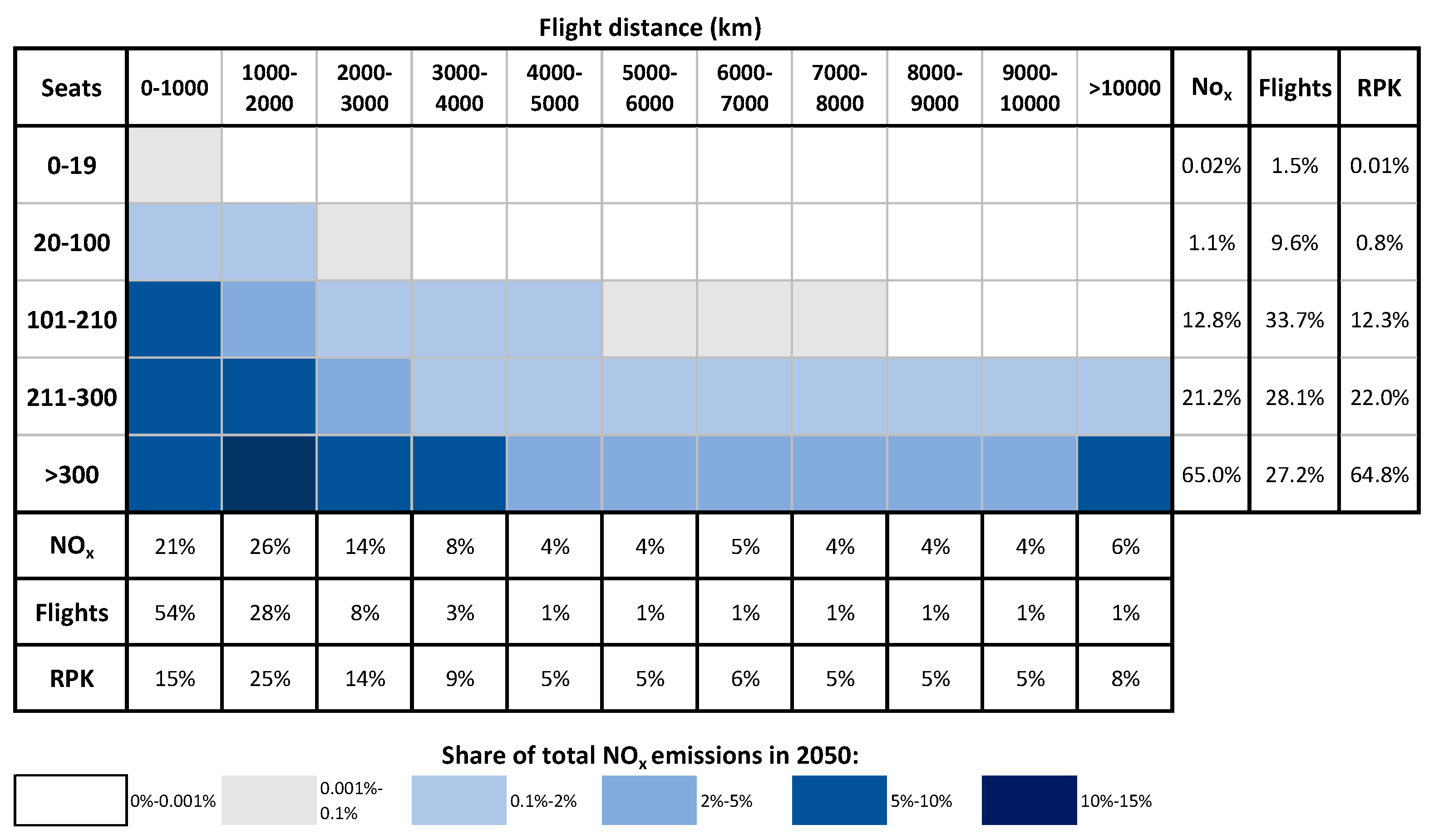
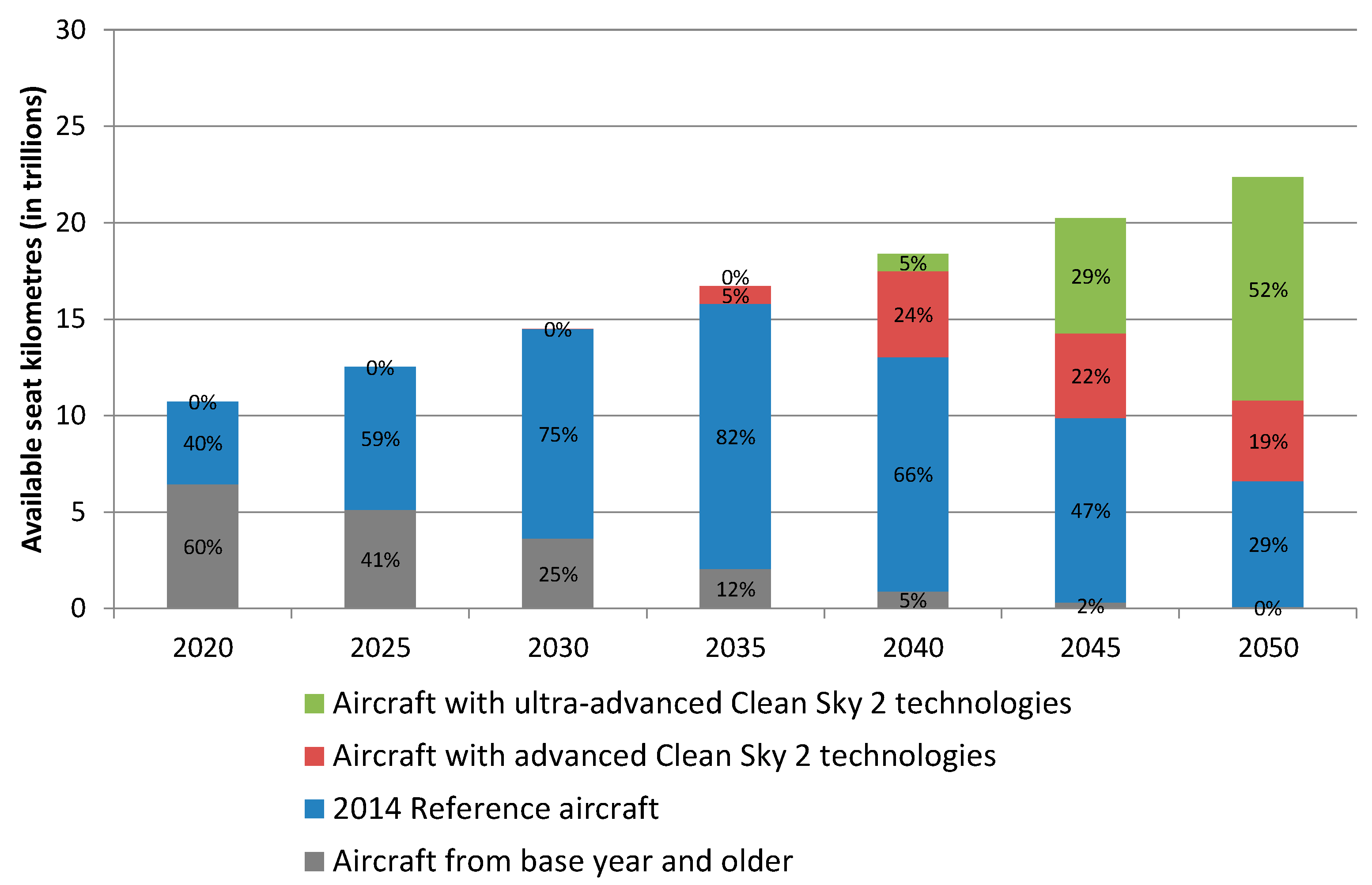
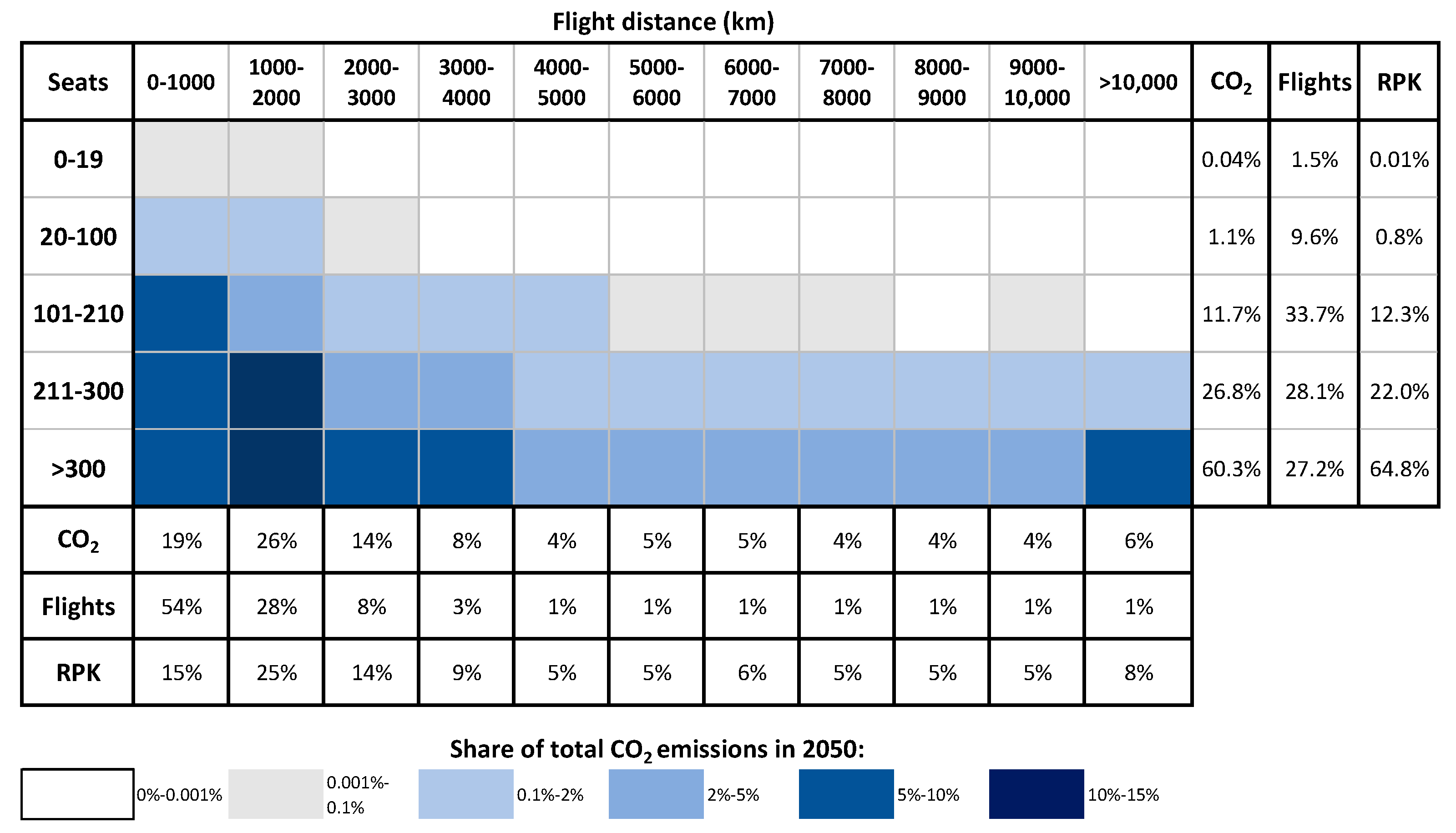
3.3. Aircraft Emissions
4. Discussion and Conclusions
Author Contributions
Funding
Institutional Review Board Statement
Informed Consent Statement
Data Availability Statement
Conflicts of Interest
References
- Berster, P.; Gelhausen, M.C.; Wilken, D. Is increasing aircraft size common practice of airlines at congested airports? J. Air Transp. Manag. 2015, 46, 40–48. [Google Scholar] [CrossRef]
- Gelhausen, M.C.; Berster, P.; Wilken, D. Airport Capacity Constraints and Strategies for Mitigation: A Global Perspective; Academic Press: New York, NY, USA, 2019; pp. 1–327. [Google Scholar]
- Wilken, D.; Berster, P.; Gelhausen, M.C. New empirical evidence on airport capacity utilisation: Relationships between hourly and annual air traffic volumes. Res. Transp. Bus. Manag. 2011, 1, 118–127. [Google Scholar] [CrossRef] [Green Version]
- Givoni, M.; Rietveld, P. The environmental implications of airlines’ choice of aircraft size. J. Air Transp. Manag. 2010, 16, 159–167. [Google Scholar] [CrossRef]
- Pitfield, D.E.; Caves, R.E.; Quddus, M.A. Airline strategies for aircraft size and airline frequency with changing demand and competition: A simultaneous-equations approach for traffic on the north Atlantic. J. Air Transp. Manag. 2010, 16, 151–158. [Google Scholar] [CrossRef] [Green Version]
- Brueckner, J.K.; Zhang, Y. A model of scheduling in airline networks: How a hub-and-spoke system affects flight frequency, fares and welfare. J. Transp. Econ. Policy 2001, 35, 195–222. [Google Scholar]
- Gelhausen, M.C.; Berster, P.; Wilken, D. Post-COVID-19 Scenarios of Global Airline Traffic until 2040 That Reflect Airport Capacity Constraints and Mitigation Strategies. Aerospace 2021, 8, 300. [Google Scholar] [CrossRef]
- Gelhausen, M.C. Modelling the effects of capacity constraints on air travellers’ airport choice. J. Air Transp. Manag. 2011, 17, 116–119. [Google Scholar] [CrossRef]
- Gudmundsson, S.V.; Paleari, S.; Redondi, S. Spillover effects of the development constraints in London Heathrow Airport. J. Transp. Geogr. 2014, 35, 64–74. [Google Scholar] [CrossRef]
- Redondi, R.; Gudmundsson, S.V. Congestion spill effects of Heathrow and Frankfurt airports on connection traffic in European and Gulf hub airports. Transp. Res. Part A Policy Pract. 2016, 92, 287–297. [Google Scholar] [CrossRef]
- Dennis, N. Airline hub operations in Europe. J. Transp. Geogr. 1994, 2, 219–233. [Google Scholar] [CrossRef]
- Airports Commission. Airports Commission: Final Report; Airports Commission: London, UK, 2015. [Google Scholar]
- Airbus. Global Market Forecast 2021–2040; Airbus: Blagnac, France, 2021. [Google Scholar]
- Boeing. Commercial Market Outlook 2021–2040; Boeing: Seattle, WA, USA, 2021. [Google Scholar]
- International Civil Aviation Organization (ICAO). ICAO Long-Term Traffic Forecast—Passenger and Cargo; ICAO: Montreal, QC, Canada, 2016. [Google Scholar]
- Harvey, D. Airline passenger traffic patterns within the United States. J. Air Law Commer. 1951, 18, 157–165. [Google Scholar]
- Grosche, T.; Rothlauf, F.; Heinzl, A. Gravity models for airline passenger volume estimation. J. Air Transp. Manag. 2007, 13, 175–183. [Google Scholar] [CrossRef]
- Tusi, W.H.K.; Fung, M.K.Y. Analysing passenger network changes: The case of Hong Kong. J. Air Transp. Manag. 2016, 50, 1–11. [Google Scholar]
- Matsumoto, H. International urban systems and air passenger and cargo flows: Some calculations. J. Air Transp. Manag. 2004, 10, 241–249. [Google Scholar] [CrossRef] [Green Version]
- Shen, G. Reverse-fitting the gravity model to inter-city airline passenger flows by an algebraic simplification. J. Transp. Geogr. 2004, 12, 219–234. [Google Scholar] [CrossRef]
- Bhadra, D.; Kee, J. Structure and dynamics of the core US air travel markets: A basic empirical analysis of domestic passenger demand. J. Air Transp. Manag. 2008, 14, 27–39. [Google Scholar] [CrossRef]
- Endo, N. International trade in air transport services: Penetration of foreign airlines into Japan under the bilateral aviation policies of the US and Japan. J. Air Transp. Manag. 2007, 13, 285–292. [Google Scholar] [CrossRef]
- Hazledine, T. Border effects for domestic and international Canadian passenger air travel. J. Air Transp. Manag. 2009, 15, 7–13. [Google Scholar] [CrossRef]
- Alexander, D.W.; Merkert, R. Challenges to domestic air freight in Australia: Evaluating air traffic markets with gravity modelling. J. Air Transp. Manag. 2017, 61, 41–52. [Google Scholar] [CrossRef]
- Alexander, D.W.; Merkert, R. Applications of gravity models to evaluate and forecast US international air freight markets post-GFC. Transp. Policy 2021, 104, 52–62. [Google Scholar] [CrossRef]
- Baier, F.; Berster, P.; Gelhausen, M.C. Global cargo gravitation model: Airports matter for forecasts. Int. Econ. Econ. Policy 2022, 19, 219–238. [Google Scholar] [CrossRef]
- Sabre AirVision Market Intelligence. Data Based on Market Information Data Tapes (MIDT). Available online: https://www.sabre.com/products/market-intelligence/ (accessed on 8 November 2021).
- Silva, J.M.C.S.; Tenreyro, S. The log of gravity. Rev. Econ. Stat. 2006, 88, 641–658. [Google Scholar] [CrossRef] [Green Version]
- Wilken, D.; Berster, P.; Gelhausen, M.C. Airport choice in Germany: New empirical evidence of the 2003 German air traveller survey. Airpt. Manag. 2007, 1, 165–179. [Google Scholar]
- Mason, K.J. Corona Markiert Eine Zäsur Bei Geschäftsreisen. Available online: https://www.airliners.de/airline-geschaeftsmodelle-88-corona-markiert-zaesur-geschaeftsreisen/61658 (accessed on 23 August 2021).
- Charnes, A.; Cooper, W.W.; Rhodes, E. Measuring the efficiency of decision-making units. Eur. J. Oper. Res. 1978, 2, 429–444. [Google Scholar] [CrossRef]
- Cooper, W.W.; Seiford, L.M.; Tone, K. Data Envelopment Analysis—A Comprehensive Text with Models, Applications, References and DEA-Solver Software; Springer: New York, NY, USA, 2007. [Google Scholar]
- Markov, A.A. An Example of Statistical Investigation of the Text Eugene Onegin Concerning the Connection of Samples in Chains. Sci. Context 2006, 19, 591–600. [Google Scholar] [CrossRef] [Green Version]
- McFadden, D. Conditional Logit Analysis of Qualitative Choice Behavior. In Frontiers in Econometrics; Zarembka, P., Ed.; Academic Press: New York, NY, USA, 1974. [Google Scholar]
- Ben-Akiva, M.; Lerman, S.R. Discrete Choice Analysis; MIT Press: Cambridge, MA, USA, 1985. [Google Scholar]
- Gelhausen, M.C.; Berster, P.; Wilken, D. Do airport capacity constraints have a serious impact on the future development of air traffic? J. Air Transp. Manag. 2013, 28, 3–13. [Google Scholar] [CrossRef]
- Wei, W.; Hansen, M. Impact of aircraft size and seat availability on airlines’ demand and market share in duopoly markets. Transp. Res. Part E Logist. Transp. Rev. 2005, 41, 315–327. [Google Scholar] [CrossRef]
- Presto, F.; Gollnick, V.; Lütjens, K. Fleet upgauging and reducing flight frequency. J. Air Transp. 2022, 30, 23–36. [Google Scholar] [CrossRef]
- Kölker, K.; Bießlich, P.; Lütjens, K. From passenger growth to aircraft movements. J. Air Transp. Manag. 2016, 56, 99–106. [Google Scholar] [CrossRef]
- Givoni, M.; Rietveld, P. Airline’s choice of aircraft size—Explanations and implications. Transp. Res. Part A 2009, 43, 500–510. [Google Scholar] [CrossRef]
- Bhadra, D. Choice of aircraft fleets in the U.S. domestic scheduled air transportation system: Findings from a multinomial logit analysis. J. Transp. Res. Forum 2005, 44, 143–162. [Google Scholar] [CrossRef]
- Pai, V. On the factors that affect airline flight frequency and aircraft size. J. Air Transp. Manag. 2010, 16, 169–177. [Google Scholar] [CrossRef] [Green Version]
- Bhadra, D. Choice of aircraft fleets in the US NAS: Findings from a multinomial logit analysis. In Proceedings of the 3rd AIAA Aviation Technology, Integration, and Operations Conference, Denver, CO, USA, 17–19 November 2003. [Google Scholar]
- Bhadra, D. Demand for Air Travel in the United States: Bottom-Up Econometric Estimation and Implications for Forecasts by Origin-Destination Pairs. In Proceedings of the 2nd AIAA Aviation Technology, Integration, and Operations Conference, Los Angeles, CA, USA, 1–3 October 2002. [Google Scholar]
- Cirium. Fleets Analyzer. Available online: https://www.cirium.com/products/views/fleets-analyzer/ (accessed on 8 November 2021).
- Official Airline Guide (OAG). Flight Schedules. Available online: https://www.oag.com/ (accessed on 8 November 2021).
- Flightglobal. Innovata Flight Schedules. Available online: https://www.flightglobal.com/ (accessed on 8 November 2021).
- International Civil Aviation Organization (ICAO). Annual Report of the Council (Doc 9916). 2009. Available online: https://www.icao.int/publications/Documents/9916_en.pdf (accessed on 22 February 2022).
- International Civil Aviation Organization (ICAO). Annual Report of the Council, Presentation of 2016 Air Transport Statistical Results. 2017. Available online: https://www.icao.int/annual-report-2016/Pages/the-world-of-air-transport-in-2016-statistical-results.aspx (accessed on 22 February 2022).
- Flightradar24. Live Air Traffic. Available online: https://www.flightradar24.com/50.83,6.91/6 (accessed on 8 November 2021).
- Eurocontrol. Automatic Dependent Surveillance–Broadcast Airborne Equipage Monitoring. Available online: https://www.eurocontrol.int/service/adsb-equipage (accessed on 22 February 2022).
- Lissys. Piano-X. Available online: https://www.lissys.uk/PianoX.html (accessed on 8 November 2021).
- Dons, J.; Mariens, J.; O’Callaghan, G.D. Use of Third-Party Aircraft Performance Tools in the Development of the Aviation Environmental Design Tool (AEDT); Report of the U.S. Department of Transportation, Research and Innovative Technology Administration; John A. Volpe National Transportation Systems Center, Environmental Measurement and Modeling Division: Washington, NJ, USA, 2011.
- Senzig, D.A.; Dons, J.; Mariens, J.; O’Callaghan, G.D.; Iovinelli, R.J. Extending Aircraft Performance Modeling Capabilities in the Aviation Environmental Design Tool (AEDT); Report of the John A. Volpe National Transportation Systems Center; Federal Aviation Administration—Office of Environment and Energy: Washington, NJ, USA, 2011.
- DuBois, D.; Paynter, G.C. Fuel Flow Method2 for estimating aircraft emissions. SAE Int. J. Aerosp. 2006, 115, 1–14. [Google Scholar]
- Airbus. Global Market Forecast 2019–2038; Airbus: Blagnac, France, 2019. [Google Scholar]
- Boeing. Commercial Market Outlook 2019–2038; Boeing: Seattle, WA, USA, 2019. [Google Scholar]
- Grimme, W.; Maertens, S.; Bingemer, S.; Gelhausen, M.C. Estimating the market potential for long-haul narrowbody aircraft using origin-destination demand and flight schedules data. Transp. Res. Procedia 2021, 52, 412–419. [Google Scholar] [CrossRef]
- Wilken, D.; Berster, P.; Gelhausen, M.C. Analysis of demand structures on intercontinental routes to and from Europe with a view to identifying potential for new low-cost services. J. Air Transp. Manag. 2016, 56B, 79–90. [Google Scholar] [CrossRef]


| Aircraft Seat Class | Number of Aircraft in 2014 |
|---|---|
| 1–19 Seats | 1885 |
| 20–50 Seats | 2424 |
| 51–70 Seats | 1111 |
| 71–85 Seats | 1240 |
| 86–100 Seats | 148 |
| 101–125 Seats | 1359 |
| 126–150 Seats | 3346 |
| 151–175 Seats | 3496 |
| 176–210 Seats | 5273 |
| 211–300 Seats | 2144 |
| 301–400 Seats | 1435 |
| 401–500 Seats | 156 |
| Total | 24,017 |
| Total >19 Seats | 22,132 |
| Aircraft Type | Active Fleet—Cirium Fleets Analyzer | Estimated Number of Aircraft Based on Innovata Schedule | % Deviation |
|---|---|---|---|
| Airbus A320 Family | 7893 | 7997 | 1.3% |
| Airbus A330 | 1,209 | 1108 | −8.4% |
| Airbus A340 | 135 | 106 | −21.3% |
| Airbus A350 | 281 | 315 | 12.0% |
| Airbus A380 | 231 | 220 | −4.6% |
| ATR 42/72 | 877 | 720 | −17.9% |
| Boeing 737 | 6827 | 6623 | −3.0% |
| Boeing 747 | 128 | 130 | 1.8% |
| Boeing 757 | 352 | 261 | −25.7% |
| Boeing 767 | 418 | 290 | −30.6% |
| Boeing 777 | 1255 | 1257 | 0.2% |
| Boeing 787 | 803 | 836 | 4.1% |
| Bombardier CRJ | 1227 | 1078 | −12.2% |
| Embraer E-Series | 1397 | 1378 | −1.4% |
| deHavilland Dash 8 | 830 | 639 | −23.0% |
| Total | 23,863 | 22,957 | −3.8% |
| Original CS2 Reference Aircaft | ICAO Seat Category | CS2 Reference Aircraft |
|---|---|---|
| X | 1–19 | Do228 |
| 20–50 | ATR42-500 | |
| X | 51–70 | CASA C295 Civil (2014 Multi-Mission) |
| 71–85 | Bombardier Dash-8-400 | |
| X | 86–100 | ATR72 Scaled to 90 Seats |
| 101–125 | Embraer E195 | |
| X | 126–150 | Airbus A220-300 |
| 151–175 | Airbus A320neo | |
| X | 176–210 | Airbus A321neo (SMR 2014 ref) |
| 211–300 | Boeing 787-8 | |
| X | 301–400 | Airbus A350-900 (LR 2014 ref) |
| 401–500 | Airbus A380-800 (up to 2021)/Boeing 777-9 (from 2022) |
| Conceptual Aircraft/Air Transport Type | Reference Aircraft | Window 1 | ∆CO2 | ∆NOx | ∆ Noise | Target 2 TRL @ CS2 Close |
|---|---|---|---|---|---|---|
| Advanced Long-range (A-LR) | LR 2014 ref | 2030 | 20% | 20% | 20% | 4 |
| Ultra advanced Long-range (UA-LR) | LR 2014 ref | 2035+ | 30% | 30% | 30% | 3 |
| Advanced Short/Medium-range (A-SMR) | SMR 2014 ref | 2030 | 20% | 20% | 20% | 5 |
| Ultra-advanced Short/Medium-range (UA-SMR) | SMR 2014 ref | 2035+ | 30% | 30% | 30% | 4 |
| Innovative Turboprop (TP), 130 Pax | 2014 130 Pax ref | 2035+ | 19 to 25% | 19 to 25% | 20 to 30% | 4 |
| Advanced Turboprop (A-TP), 90 Pax | 2014 TP ref | 2025+ | 35 to 40% | >50% | 60 to 70% | 5 |
| Regional Multi-Mission TP, 70 Pax | 2014 Multi-mission | 2025+ | 20 to 30% | 20 to 30% | 20 to 30% | 6 |
| 19-Pax Commuter | 2014 19 Pax a/c | 2025 | 20% | 20% | 20% | 4-5 |
| Original CS2 Aircraft | Aircraft Scenario Category | ICAO Seat Category | Reference Aircraft | CS2 Aircraft Type | Entry into Service in Forecast Model | Out of Production |
|---|---|---|---|---|---|---|
| x | Reference | 1–19 | 2014 Pax a/c | 19-Pax Reference Aircraft | 2014 | 2029 |
| x | CS2 | 1–19 | 19-Pax Commuter | 2030 | 2050 | |
| Reference | 20–50 | ATR42-500 | 2014 | 2029 | ||
| CS2 | 20–50 | ATR42-500 Advanced | 2030 | 2050 | ||
| x | Reference | 51–70 | 2014 Multi-Mission | CASA C295 Civil | 2014 | 2029 |
| x | CS2 | 51–70 | Regional Multi-Mission TP 70 seats | 2030 | 2050 | |
| Reference | 71–85 | Bombardier Dash-8-400 | 2014 | 2029 | ||
| CS2 | 71–85 | Bombardier Dash-8-400 Advanced | 2030 | 2050 | ||
| x | Reference | 86–100 | 2014 TP ref | ATR72 Scaled to 90 seats | 2014 | 2029 |
| x | CS2 | 86–100 | Advanced TP90 | 2030 | 2050 | |
| Reference | 101–125 | Embraer E195 | 2014 | 2020 | ||
| CS2 | 101–125 | Embraer E195–E2 | 2021 | 2034 | ||
| CS2 | 101–125 | A-SMR-Embraer E195 | 2035 | 2039 | ||
| CS2 | 101–125 | UA-SMR-Embraer E195 | 2040 | 2050 | ||
| x | Reference | 126–150 | 2014 130 Pax ref | Airbus A220-300 | 2014 | 2039 |
| x | CS2 | 126–150 | Innovative Turboprop | 2040 | 2050 | |
| Reference | 151–175 | Airbus A320neo | 2014 | 2034 | ||
| CS2 | 151–175 | A-SMR-Airbus A320neo | 2035 | 2039 | ||
| CS2 | 151–175 | UA-SMR-Airbus A320neo | 2040 | 2050 | ||
| x | Reference | 176–210 | SMR 2014 ref | Airbus A321neo | 2014 | 2034 |
| x | CS2 | 176–210 | A-SMR | 2035 | 2039 | |
| x | CS2 | 176–210 | UA-SMR | 2040 | 2050 | |
| Reference | 211–300 | Boeing 787-8 | 2014 | 2034 | ||
| CS2 | 211–300 | A-LR-Boeing 787-8 | 2035 | 2039 | ||
| CS2 | 211–300 | UA-LR-Boeing 787-8 | 2040 | 2050 | ||
| x | Reference | 301–400 | LR 2014 ref | Airbus A350-900 | 2014 | 2034 |
| x | CS2 | 301–400 | Airbus A350-900neo | 2035 | 2039 | |
| x | CS2 | 301–400 | UA-LR | 2040 | 2050 | |
| Reference | 401–500 | Airbus A380-800 | 2014 | 2021 | ||
| Reference | 401–500 | Boeing 777-9 | 2022 | 2034 | ||
| CS2 | 401–500 | Airbus A350-2000neo | 2035 | 2039 | ||
| CS2 | 401–500 | UA-LR | 2040 | 2050 |
| Year | High Scenario | Low Scenario | ||
|---|---|---|---|---|
| ∆CO2 | ∆NOx | ∆CO2 | ∆NOx | |
| 2035 CS2 vs. Reference | −0.8% | −1.9% | −0.8% | −1.9% |
| 2040 CS2 vs. Reference | −4.6% | −12.0% | −4.1% | −10.2% |
| 2045 CS2 vs. Reference | −10.1% | −23.0% | −9.2% | −20.1% |
| 2050 CS2 vs. Reference | −14.6% | −31.0% | −13.8% | −29.0% |
Publisher’s Note: MDPI stays neutral with regard to jurisdictional claims in published maps and institutional affiliations. |
© 2022 by the authors. Licensee MDPI, Basel, Switzerland. This article is an open access article distributed under the terms and conditions of the Creative Commons Attribution (CC BY) license (https://creativecommons.org/licenses/by/4.0/).
Share and Cite
Gelhausen, M.C.; Grimme, W.; Junior, A.; Lois, C.; Berster, P. Clean Sky 2 Technology Evaluator—Results of the First Air Transport System Level Assessments. Aerospace 2022, 9, 204. https://doi.org/10.3390/aerospace9040204
Gelhausen MC, Grimme W, Junior A, Lois C, Berster P. Clean Sky 2 Technology Evaluator—Results of the First Air Transport System Level Assessments. Aerospace. 2022; 9(4):204. https://doi.org/10.3390/aerospace9040204
Chicago/Turabian StyleGelhausen, Marc Christopher, Wolfgang Grimme, Alf Junior, Christos Lois, and Peter Berster. 2022. "Clean Sky 2 Technology Evaluator—Results of the First Air Transport System Level Assessments" Aerospace 9, no. 4: 204. https://doi.org/10.3390/aerospace9040204
APA StyleGelhausen, M. C., Grimme, W., Junior, A., Lois, C., & Berster, P. (2022). Clean Sky 2 Technology Evaluator—Results of the First Air Transport System Level Assessments. Aerospace, 9(4), 204. https://doi.org/10.3390/aerospace9040204