1. Introduction
The development of microsatellites leads to a general trend in Networking with LEO mega-constellations. Many countries and companies have proposed building this type of constellation, such as OneWeb and Starlink in the United States [
1]. Of these, the Starlink communications constellation of 12,000 satellites is expected to be constructed around 2025, and accumulated to 42,000 satellites afterward [
2].
Compared with the traditional middle and high Earth orbit navigation constellations, the LEO mega-constellations are characterized by low orbit height, dense satellite distribution, large perturbation, and high requirements for station position maintenance. Although the relative phase between satellites will not drift in constellations with the same value of mean elements, due to errors in the measurement data, dynamic model, solution algorithm, actuator, and other factors, the constellation configuration will be out of order in the uncontrolled state, leading to a high risk of collisions within the constellations.
To investigate how much the relative phase between satellites in the same orbital plane in the LEO mega-constellations will be drifted by the perturbations, it is critical to first point out the nominal value of the constellation design. From the semi-analytic theory [
3], the satellite orbits can be described by their initial mean elements. If the initial mean elements of the constellation are identical, the relative phases within the constellation will not theoretically diverge. So, the constellation nominal values can be considered a set of mean elements. Accordingly, the problem of phase evolution affected by perturbations can be viewed as the initial uncertainties propagation of the constellation: how to establish the mapping relationship of the terminal state to the initial state. The initial state is the deviation of the position velocity of the two satellites from the nominal design value, and the terminal state is the deviation of the relative phase of the two satellites from the design nominal value after a while.
As widely recognized, orbit propagation is a fundamental problem in astrodynamics. There are three main approaches for modeling orbit propagation [
4]: the numerical approach, analytical approach, and semi-analytical approach. The numerical approach [
5,
6] has high precision and is suitable for scenarios with complex mechanical environments, but consumes more computational resources. The analytical approach [
7] is developed on Brouwer’s perturbation solutions [
8,
9], using an approximate analytical solution instead of the original ordinary differential equations of motion, preserving the main features of the perturbation while neglecting higher-order small terms. The analytical approach makes the calculation much more efficient while losing some accuracy. The semi-analytical approach [
10,
11] mixes the analytical and numerical approaches’ advantages, classification of perturbation solutions into long-term, long-period, and short-period terms according to perturbation characteristics. Bezděk [
12] presents the computational efficiency strength of the semi-analytical approach in long-term dynamics. Golikov [
13] presents a dynamic approach of satellite formation flights based on the THEONA semi-analytical theory with arbitrary values of the eccentricity.
For general stochastic dynamical systems, the evolution equation of the probability density over time satisfies the Fokker–Planck equation [
14] (FPE), while for orbital dynamical systems with high dimensionality (6 dimensions) and nonlinear perturbations, the FPE solution becomes very tough. Thus, the probability density function (PDF) evolution often requires the assumption of local linearization and only the lower order moments (e.g., mean and covariance matrices) are analyzed. Currently, nonlinear uncertainty propagation approaches include polynomial chaos expansions [
15], state transition tensor approaches [
16,
17], differential algebra approaches [
18,
19], and Gaussian mixture model approaches [
20]. Most of the theories of uncertainty propagation are, however, focused on explaining the behavior of medium and high Earth orbit navigation constellations, seldom involving LEO mega-constellations. A well-known and robust approach used to study the uncertainty propagation problem is the Monte Carlo simulation [
21], and the distribution of terminal states is obtained through the steps of randomly taking a large number of samples, high-precision simulation, and statistical analysis. The numerical approach-based Monte Carlo simulation has a long computation time and high hardware requirements. A possible solution to the problem at hand is applying the semi-analytical dynamics model, which does not need to propagate the orbital elements of the satellite or the position and velocity vectors of the satellite to obtain the position information of the satellite at a specific time and therefore has a smaller computational memory and computational load [
22].
This paper aims to develop an overarching framework to reveal the uncertainty propagation law of the phase of LEO mega-constellations. The perturbation solution is modeled in
Section 2.
Section 3 describes the Monte Carlo uncertainty propagation approach.
Section 4 carries out a numerical simulation. Conclusions are drawn in
Section 5.
2. Modeling the Orbital Dynamics
In the geocentric equatorial inertial coordinate systems, the orbit motion of a satellite can be reduced to a perturbed two-body problem, and the motion equation is a set of ordinary differential equations [
23]
where
r and
are the position vectors and velocity vectors of the satellite,
t is the propagation time,
is the two-body motion acceleration of the central body,
is the perturbation acceleration, and
is a small parameter. Utilizing asymptotic expansion and other approaches, the power series form solution of small parameter
can be constructed [
24], such as
where
are the classical orbital elements: semimajor axis, eccentricity, inclination, right ascension of the ascending node, argument of perigee, and mean anomaly at epoch, respectively. By substituting the formal solution into the original perturbed motion equation and comparing the coefficients of the same power
at both ends, the perturbation solutions of each order can be obtained. By the average approach, the perturbation solutions can be divided into secular terms, long-period terms, and short-period terms according to forms of presentation.
Among them,
is the epoch time,
are the osculating elements at time
,
is the initial mean elements,
is the mean elements at time
t,
,
n is the mean motion of satellite in two body,
makes up the secular terms,
consists of the long period terms, and
consists of the short-period terms. Besides this, Equation (
3) describes the identity mapping between mean elements and the osculating elements, which can be solved by numerical algorithm such as Newton iteration [
25].
LEO constellations are mainly affected by atmospheric drag and non-spherical Earth gravity. The first-order and second-order secular term of
, the first-order long-period term of
, the first-order short-period term of
, and the secular term of atmospheric drag are involved in the semi-analytical dynamic model. It should be noted that in order to avoid the abnormal matrix caused by the large numerical difference among the Keplerian elements, distance and time variables need to be normalized by
and
, where
is the Earth’s equatorial radius and
is the Earth’s gravitational constant. Thus, the mean motion
n is expressed by
. Detailed semi-analytical solutions are recorded in [
26].
2.1. Earth Non-Spherical Gravity Perturbation Solution
The bulge at equator exerts a pull on the satellite toward the equatorial plane. Whether the satellite is above or below the equatorial plane, the orbital plane will move toward the equator and make a precession motion [
27]. The main perturbation solutions of
are listed below.
The first-order secular terms of
are
The second-order secular terms of
are
The first-order short-period terms of
are
The first-order long-period terms of
are
By substituting short-period terms (Equation (
6)) and long-period terms (Equation (
7)) into the first equation in Equation (
3), the mean elements and osculating elements conversion can be realized.
2.2. Perturbation Solution of Atmospheric Drag
The secular terms of atmospheric drag are
where
is the atmospheric density scale height rate,
is the Bessel function of the first type of virtual variables, and variable
z abides by
Other intermediate quantities are given as follows:
where
S is the cross-sectional reference area,
m is the satellite mass,
is the drag coefficient,
is the Earth spin rate, the elements
are the initial Keplerian elements,
and
are atmospheric density and the density scale height of the initial perigee of the satellite orbit, and
and
are the position and velocity at the same point.
3. Uncertainty Propagation Approach of Constellation Phase
The uncertainty propagation problem satisfying the dynamic constraints Equation (
1) can be described as: Given the initial state
and the PDF
of the initial state deviation
, find the PDF
of the state
of the dynamical system at any moment or its statistical moments of each order. Generally only the first two order statistical moments of the deviation
, i.e., the mean and covariance matrix, are of interest.
Because controllers, thrusters, and observers have a direct influence on the instantaneous state of the satellite, and the terminal state quantity we are interested in is the mean elements of the satellite, the samples are generated on the satellite’s osculating trajectory, and the terminal samples appear around the mean trajectory. Therefore, the initial state errors are modeled as a probability distribution of three-dimensional position/velocity components
of the two co-plane satellites at the moment
. Since the short period effect is removed by averaging in the dynamics model, only long and long-period effects are retained, so the different initial positions of satellites in one orbital plane do not influence the evolution process. It means that the relative phase evolution of any two co-plane satellites can represent the divergence of this whole orbital plane. The relative phase
of the two satellites after time
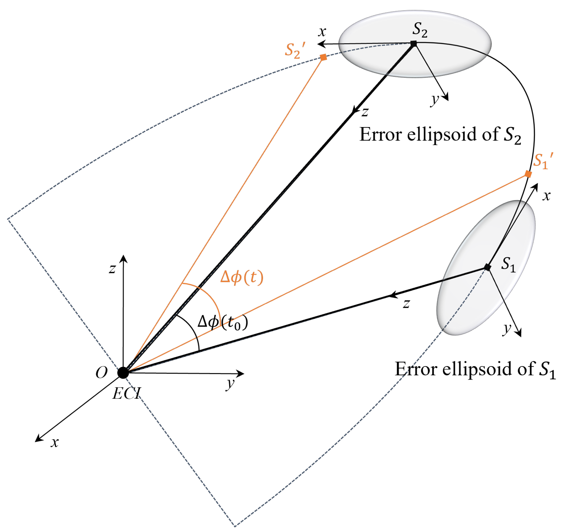
t is chosen as the terminal state quantity. The schematic diagram of two co-plane satellites’ uncertainty propagation is shown in
Figure 1. Since the orbits of LEO mega-constellations tend to be near-circular, the argument of latitude
is used to characterize the phase angle of a satellite. The evolution of the initial state to the terminal state involves, in turn, the transformation of the position-velocity components to the osculating elements, the transform between osculating elements and mean elements, and the semi-analytical propagation. The whole physical process shows strong nonlinearities, so the Monte Carlo is an appropriate analysis approach.
3.1. Semi-Analytical-Based Monte Carlo Simulation Design
Without loss of generality, we assume that the initial state quantities of each co-planar satellite in the satellite orbit coordinate system follow a three-dimensional Gaussian distribution with zero mean
, and the components are independent of each other. Then, the joint Gaussian PDF is
where the covariance matrix of the initial position velocity errors
and
are
where diag represents a diagonal matrix with the entries on the diagonal.
To further simplify the problem, Monte Carlo simulations are performed in two hypothetical cases: Case I, where both two satellites have only initial position errors, and the position standard deviation is ; Case II, where both two satellites have only velocity errors, and the velocity error is noted as .
A number of N samples are generated, and the samples are then propagated over time individually, and the a posteriori uncertainty distribution is reconstructed from the integrated samples. Multiple sets of position (velocity) standard deviations () with orbital propagation time t are taken, and multiple Monte Carlo simulations are performed to count the first two order moments of the relative phase distribution, which are the mean and standard deviation. Combining hypothesis testing and surface fitting, an approximate mapping between the initial covariance and the terminal covariance can be obtained.
It should be noted that since the relative phase is a directional statistic, and
and
are identical angles, so that for example
is not a sensible mean of
and
. To avoid this error, the directional mean
and the directional standard deviation
of the directional quantity
should be calculated by Equation (
16) [
28]
where the center of mass
of the directional statistic is
and the mean resultant length is
3.2. Hypothesis Testing of Monte Carlo Simulations Results
The overall terminal phase quantities obtained from the Monte Carlo simulation are denoted as
. The Gaussian distribution remains normal after propagation by the linear or linearized dynamic equations [
29], while the two-body motion plays a dominant role in the orbital dynamics, and the
regimens and the atmospheric drag regimens are small quantities. Thus, the terminal quantities can be considered to obey the same Gaussian distribution
. In order to test whether the mean
of the relative phase distribution is zero, a statistical hypothesis test is required [
30]. Two mutually opposing hypotheses are made for
The test statistic distinguishing the first hypothesis from the alternative hypothesis is
z value and is given by
The significance level is given and the standard Gaussian distribution table is queried to determine the rejection domain. If is satisfied, the hypothesis is accepted (the opposing hypothesis is rejected), i.e., it is considered that, ideally, two co-plane satellites will not diverge or cluster under perturbations; if , the hypothesis is accepted (the hypothesis is rejected), i.e., it is considered that ideally the non-uncertainty case, the relative phase will also have drifted.
3.3. Product-Based Least-Squares Surface FITTING Approach
Multiple sets of Monte Carlo simulations with different orbital propagation times
t and position (velocity) standard deviations
(
) are selected. The time series is denoted as
(days), the position or velocity standard deviation series is denoted as
(
or
), the standard deviation of the phase difference obtained by the Monte Carlo approach is denoted as
(
), and
are all row vectors, which approximately form a three-dimensional surface. The set of functions
is used as the basis function for the product-type least-squares fit [
31], where
Construct a surface with
as parameter, which can be expressed as
where, the coefficient
is a matrix form given by
with
In this way, an approximate function of the standard deviation of the initial position velocity and the standard deviation of the phase difference can be obtained.
4. Numerical Simulations and Results
We will now demonstrate the method for a specific problem. Because the Starlink constellation is a typical LEO mega-constellation with great research significance, we choose the orbit and mechanical environmental parameters of Starlink for simulation. Take into consideration the satellite with mean Keplerian elements as shown in
Table 1 and mechanical environmental parameters as shown in
Table 2 to conduct Monte Carlo simulations. Orbital and structural parameters of Starlink satellites can be found in SpaceX’s FCC documents (such as 36 FCC Rcd 7995 (11)(2021)). In our simulations, the semi-analytical approach shows a strong advantage in computing efficiency. On a PC equipped with i7-1065G7 CPU 1.30 GHz, the numerical and the semi-analytical approach respectively take 4.258
and 0.103
under
and atmospheric drag for the 7-day orbit prediction.
Without loss of generality, the initial position and velocity uncertainty of the satellite is assumed to be Gaussian distributed, and are defined in the geocentric inertial coordinate system. The mean is zero and the covariance matrix is
Four thousand points are distributed to be consistent with the initial uncertainty, generated and propagated using the averaged
and atmosphere drag dynamics, referring to the second equation of Equation (
3). The secular terms of
and atmosphere drag are the same as Equations (
4), (
5), and (
8). The conversion between osculating elements and mean elements abides by the first equation of Equation (
3), and short-period terms and long-period terms are described in Equations (
6) and (
7).
Figure 2 shows initial points distribution before and after conversion from osculating elements to mean elements. The mean track propagated in averaged
and atmosphere drag dynamics is marked as a green line, while the osculating track propagated in full dynamics—which includes short-period and long-period terms besides secular terms—is marked as an orange line. To better display the size of the uncertainty ellipsoid, the absolute position of the points is subtracted from the nominal position, and denoted by
. It can be seen that it is the conversion between osculating elements and mean elements that makes the distribution of sample points show strong nonlinearity at initial moments.
Figure 3 shows points distribution after different revolutions up to 100 orbits, which is about 6.2 days. The samples are gradually correlated with the mean trajectory as the propagation time progresses. After 1 orbit period, the shape of points takes on a shuttle shape. Hence, it is reasonable to assume that the position nonlinearity becomes weaker after several revolutions. The argument of latitude of a satellite is Gaussian distribution after going through the same revolutions.
Table 3 shows the first two order moments of the relative phase of two co-plane satellites in the constellation,
z value of hypothesis test Equation (
20) and whether
should be accepted are also presented in this table.
There is only a difference in relative position between the two satellites, and other initial mean elements of them are the same. When the significance level of hypothesis test is given as 0.05, the z value of the two-sided test is 1.96. Thus, the hypothesis is rejected in the beginning and is accepted after 1 orbit, because the standard deviation is growing faster than the mean over time. As a consequence, the phase of two co-plane satellites can also be considered as a Gaussian distribution with zero mean as propagation time goes by.
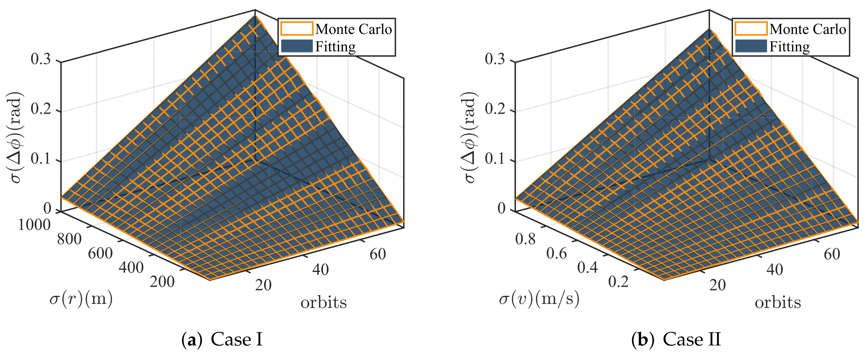
In the multi-group MC simulation, the total number of samples per group is set to be 4000, the propagation time is chosen as days, the position standard deviation is , and the velocity standard deviation is . There are a total of 625 groups in each case and are parallel computed.
The standard deviation surfaces of the relative phase in two cases are shown in
Figure 4, and the least-squares surface fitting parameters are shown in
Table 4. Taking
, the
z value of the two-sided test is 2.58, and the acceptance rate of hypothesis
reaches 96% in both two scenarios, indicating that our assumption is logical.
Since the fitting relationship of the initial standard deviation to the terminal standard deviation has been obtained, we can easily make deviation forecasts for controllers with known error magnitudes, or infer the control and observation error of a constellation backward from its deviation evolution. For example, if two co-plane satellites have an initial uncertainty of 100 standard deviation in three-dimensional position, after 20 orbits, the relative phase appears an uncertainty of standard deviation, which could be also be caused by 0.109 three-dimensional velocity errors.
5. Conclusions
In this paper, an uncertainty propagation analysis approach based on the semi-analytical dynamic approach, Monte Carlo simulation, and least-squares fitting is proposed. The overall approach shows significant benefits in terms of improving the computational efficiency of uncertainty propagation and is suitable for LEO mega-constellations scenarios. On this basis, numerical tests confirm that the probability density will become highly nonlinear after the conversion between osculating elements and mean elements, and the positions distribution of the satellite fits its mean trajectory after the initial nonlinear moment about one orbit period, leading to the phase of two co-plane satellites can be considered as a Gaussian distribution with zero mean as propagation time goes by. Ulteriorly, multi-group Monte Carlo simulations under the effect of initial normal position or velocity error and hypothesis testing verify the assumption. Finally, the initial standard deviation, propagation time, and terminal standard deviation can be described by a binary equation, which can estimate the phase error or infer initial uncertainties.
The major limitation of the present study is that the initial position and velocity errors are considered separately in two cases, but the two coexist in practice, and the other is that our approach is only suitable for low Earth orbit scenarios.


