Abstract
Fluid off-takes and complex delivery ducts are common in many engineering systems but designing them can be a challenging task. At the conceptual design phase many system parameters are open to consideration and preliminary design studies are necessary to instruct the conceptualisation process in an iterative development of design ideas. This paper presents a simple methodology to parametrically design, explore and optimise such systems at low cost. The method is then applied to an aerodynamic system including an off-take followed by a complex delivery duct. A selection of nine input variables is explored via a fractional factorial design approach that consists of three individual seven-level cubic factorial designs. Numerical predictions are characterised based on multiple aerodynamic objectives. A scaled representation of these objectives allows for a scalarisation technique to be employed in the form of a global criterion which indicates a set of trade-off geometries. This leads to the selection of a set of nominal designs and the determination of their robustness which will eventually instruct the next conceptual design iteration. The results are presented and discussed based on criterion space, design variable space and contours of several flow quantities on a selection of optimal geometries.
1. Introduction
Fluid off-takes coupled to complex duct systems are common in many engineering applications. These include, for example, engine air intakes for both aero-engines and ground vehicles, secondary air bleeds to provide cooling flows, tidal turbine intakes, distributary water channels etc. A generic description of a fluid off-take is the diversion of a portion of the mainstream flow, of the given system, via a discrete opening on a solid boundary as illustrated in Figure 1.
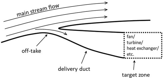
Figure 1.
Generic off-take and delivery duct.
Downstream of the off-take, depending on the application, the flow may be suitable for use directly or it may be necessary to accelerate or decelerate before delivered to the target zone. Therefore, the delivery duct can be of constant or variable cross-sectional area distribution, i.e., a nozzle or a diffuser. The target zone itself represents the region where the diverted flow is utilised. This zone may simply represent a reference section for aerodynamic evaluation or more likely the inlet to an engine, some turbomachinery, a heat exchanger, a manifold, or some other engineering component. The aerodynamic performance of the off-take and delivery duct will determine the overall performance of the application they serve. Inappropriate designs may cause flow phenomena such as flow separation, high levels of aerodynamic blockage, unacceptable total pressure loss and high levels of non-uniformity, hence careful aerodynamic design is needed.
This generic concept is studied on a specific application relating to a cooled cooling air (CCA) system on an aero gas turbine [1]. Briefly, a CCA system uses part of the bypass duct airflow to cool, via an array of heat exchangers (HX), a portion of the core engine airflow, which is then used to cool hot components in the engine core [1,2,3]. The current work considers the low pressure (LP) side of this system. This comprises an aerodynamic off-take that captures the “cooling” air from the bypass duct and a delivery duct that transfers it to the HX.
Fluid off-takes can be sub-divided in two broad categories: total off-takes and flush off-takes. In general, a total off-take will produce the best pressure recovery and aerodynamic performance [2,3,4]. This is mainly because a total off-take is operated by the total pressure of the mainstream flow as opposed to a flush off-take that in principle is operated solely by the static pressure. However, in the bypass duct of a gas turbine, the preferred option is flush or submerged off-takes as they can minimise the aerodynamic effect on the bypass stream and the associated impact in efficiency and SFC. Examples of work employing flush off-takes in the bypass duct can be found at Walker et al. [1,5] and Spanelis and Walker [6].
A parameter of importance to the current work is the location of the off-take within the bypass duct. Traditionally the preferred location is on the inner cowl surface which offers a wide surface area as well as easy access to the engine’s core. The drawback is that the quality of the ingested flow is relatively low, due to the thick boundary layers coexisting with the fan outlet guide vane (OGV) wakes. An alternative location would be the upper and lower bifurcations (the large struts in the bypass duct—Figure 2). The trend for increased bypass ratio, to enhance propulsive efficiency, leads to larger bypass ducts and consequently larger bifurcations struts. See, for instance, the work of Clemen et al. [7] who describe the design and optimisation of the bypass duct system on a large civil turbofan engine. This enlargement creates additional volume inside the struts for possible placement of air delivery ducts, hence a submerged off-take on a bifurcation strut becomes an attractive option.
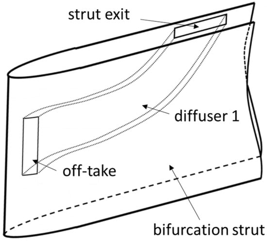
Figure 2.
Bifurcation off-take concept–sketch.
Depending on the position of the aerodynamic off-take on the bifurcation strut, the type of flow ingestion can vary between a total off-take and a flush off-take as shown in Figure 3.
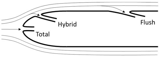
Figure 3.
Submerged off-take types on a round leading-edge surface.
For a bifurcation off-take the flow must be ducted away from the strut to the target zone and the aerodynamic and mechanical constraints add to the design challenge. In this study, the target zone for a CCA system is an array of heat exchangers located at discrete positions around the turbine casing. The velocity in the bypass duct is typically M0.5–0.6 hence, to avoid excessive total pressure losses in the HX (see Shah and Sekulic [8]) the flow captured by the off-take must be diffused. It is desirable to spread this diffusion throughout the duct system. Due to spatial constraints, some diffusion can be achieved via pre-diffusion of the captured stream-tube and some can be achieved in diffuser 1 (see Figure 2 and Figure 4). However, approximately 90% of the diffusion will need to be achieved between the strut exit and the HX. In previous work of Spanelis et al. [9] this region was comprised of two s-ducts separated by a vane. Their results suggested that flow uniformity at duct exit is maximised for designs which concentrate the aerodynamic loading (both diffusion and curvature) close to the HX. They attributed this to the beneficial effects that the HX blockage exerts on the flow immediately upstream of the HX. Therefore, as shown in Figure 4, this region is sub-divided in two components: (1) a plane diffuser referred to as “diffuser 2” which should be moderately loaded, and (2) an s-shaped manifold connected to the HX which can then be more aggressively loaded by taking advantage of the above-mentioned local pressure field near the HX. For the CCA system examined herein the target diffusion equates to an area ratio of within an overall non-dimensional length of . Where “s” denotes the stream-tube captured by the off-take and “T” is the target zone or, here, the HX inlet plane. Note that a single off-take feeds two HXs therefore, represents the combined inlet area of both.

Figure 4.
Schematic representation of the LP-CCA system.
The presented system is a conceptual design. It can be shown via the elementary timeline of a design process in Figure 5, that in an industrial environment there is a significant overlap between different design stages. The purpose of this overlap is to improve efficiency of the workforce. See for instance the description of the aircraft design process as explained by Gudmundsson [10]. More specifically, as the conceptual design stage phases out, the preliminary investigation is already in progress, which provides the opportunity to the conceptualisation team to further develop the concept. A new preliminary design iteration will then follow on the updated concept. This feedback loop continues until the design is mature enough to proceed to the next design stages. In line with the above, the general scope of this paper is to present a single step in the evolution of the above conceptual design, generalised into a suitable method to support the iterative process between conceptualisation and preliminary design space exploration.
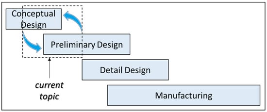
Figure 5.
Generic timeline of a design process.
At this early design phase, the engineer must seek simplifications that will not affect the leading order properties of the system. This task is far from trivial due to component interactions upstream-to-downstream and vice versa. See for example A’Barrow et al. [11] who illustrates that the presence of a diffusing off-take downstream of a compressor can have an upstream effect on the compressor and similarly the compressor’s exit conditions will also affect the performance of the diffusing off-take. Additionally, Spanelis and Walker [6] who investigated the effects of an annular bleed between the stator and the rotor of a low-pressure compressor, showed that the position of the bleed is responsible for severe flow bias in the radial direction which can reduce the OGV stall margin and alter the OGV stall topology itself. The current system can be described by a large set of closely coupled design variables which define the aerodynamic shape. Relevant examples are given by Jirásek [12] and Hamstra et al. [13], who investigated s-shaped intake ducts that employed design of experiment (DoE) techniques, a.k.a. factorial design, to obtain an optimum shape. Furthermore, the work of Yurko and Bondarenko [14], employed factorial design to examine a single annular s-duct by means of four design variables. On a previous iteration of the present conceptual design evolution, Spanelis et. al. [9] examined a double s-duct by sequentially exploring eight primary and five secondary design variables. Their findings have fed back to evolve the conceptual design to the current state by introducing new features, such as a significant elongation of the vane that separates the two heat exchangers and an independent diffusing duct segment upstream of the manifold (i.e., diffuser 2).
Further to the general scope of this paper that was stated above, the following specific objectives are set:
- (A)
- Simplify and parametrically model the conceptual design.
- (B)
- Select and evaluate a suitable approach to sample the design space.
- (C)
- Define a set of quality evaluation criteria (design objectives).
- (D)
- Develop a multi-objective characterisation methodology.
- (E)
- Characterise the design space.
- (F)
- Select and evaluate a set of nominal geometries to advance to the next stage of the design process.
In the remaining part of this paper, Section 2 provides description and justification of modelling choices, assumptions and simplifications that render this method capable to meet the above targets and objectives. Then, specific details such as the description and quantitative definition of input and output variables, as well as the numerical simulation parameters, are presented in Section 3. The results are then presented in Section 4 and Section 5 followed by a brief conclusion of this paper in Section 6.
2. Methodology
As mentioned in the introduction, this study concerns the iterative process between the conceptual and preliminary design phase of the CCA system. In this phase the availability of computational resources is limited as funding is not fully committed yet. For instance, the numerical predictions presented in this paper have been acquired as part of a single iteration of this design cycle and have only utilised a single high-performance desktop computer for less than two days. To achieve this low computational cost, several simplifications have been implemented both in the examined model and in the sampling approach. This paragraph discusses and justifies the various design choices and then quantitatively presents the selected model parameters.
2.1. Modelling Assumptions and Limitations
Typically, at this early phase in the design process it is not viable to employ physical experiments. A numerical approach is more suitable in terms of both time and cost considerations. The computational cost of a single design iteration depends on the leading order accuracy of the model. More specifically, high fidelity, three-dimensional simulations are not attractive for the exploration of a conceptual design. In this way, to maintain a balance between numerical accuracy and computational cost, a simplified two-dimensional version of the problem is considered, which is a valid approximation given that the primary flow features can be resolved in two dimensions. In terms of turbulence modelling, there is a vast range of models available in the literature, for which accuracy and computational cost are in general directly linked to one another. For this study, RANS modelling has been selected as it is an economic yet sufficiently accurate approach, that has been extensively validated for duct flows.
Furthermore, during this phase it is recommended to maximise the input variable ranges in order to identify all valuable design regions. Constraints can be set based on limits known to exist by theory or by empirical models. In this study, diffuser loading charts have been employed to limit the expansion rate of various duct components. Additionally, constraints are often set by physical objects in the environment of the system itself. For instance, here the maximum limit of the off-take opening and diffuser 1 expansion rate are set by the available space within the strut, while the width of diffuser 2 is constrained by the turbofan gearbox which is located near the strut exit.
Maximising the input variable ranges brings about an additional computational challenge. As the variable ranges increase, the probability for the observed effects to exhibit linear trends across the boundaries of the design space decreases. In fact, the results of this study revealed the existence of multiple peaks and valleys of the objective functions within the design space. Often, classical DoE engineering research uses between two and three levels per input variable. Such a low number of levels requires the creation of empirical models to correlate the limited responses observed, i.e., response surface modelling. With the increased non-linearity of the observed effects in the large design spaces considered here, a larger number of levels per variable is required (further discussed in the next sub-section).
The present study has only considered the “max take-off” condition because at this stage in the flight envelope the engines are at full thrust which is when the CCA system is mostly needed. While the concept considers the option to set a mechanical valve that regulates the flow in the system so that it can be “turned off” when not needed, other engine conditions are subject to investigation at a more matured design stage. Furthermore, this study assumes a symmetric geometry and neglects any swirl reminder exiting the bypass duct OGV. However, this is not a leading order characteristic of this system and alongside other three-dimensional flow features it is subject to optimisation in a subsequent design stage. Moreover, the configuration of the return ducting downstream of the HX is not fully decided yet. For this reason, the exit pressure and the overall loss of the cooling system are unavailable. Therefore, closure of the numerical model has been achieved here by fixing the system mass flow rate to the nominal amount for the given HX (more details in Section 3).
2.2. Sampling Approach
This subsection discusses the approach selected to sample the design space. A review on design modelling through numerical experiments has been carried out by Chen et al. [15]. Furthermore, Yondo et al. [16] presented a review of DoE and surrogate models for aerodynamic design. From these we can see that advantages of the factorial design approach compared to other design exploration and optimisation methodologies include the following:
- (a)
- It is much more efficient in the estimation of the main effects, i.e., it allows direct evaluation of the design variable interactions.
- (b)
- The complete dataset is available a priori which facilitates weighting of the multi-objective functions.
- (c)
- It is relatively simple to apply, and it does not require an expertise in advanced optimisation algorithms.
The main disadvantage, however, is the high computational cost associated with large number of design iterations, which can be a prohibitive constraint when many design variables are closely coupled to one another. Gradient-based methods are efficient in finding the true optimal solution in such problems while they can directly handle non-linear constraints. However, true optimality is not the primary objective in the conceptual design phase. The primary objective here is to identify different design families via the systematic mapping of areas of interest in the design space. Factorial design offers this attribute and with sufficiently high sampling resolution it also offers a set of perceived optimal solutions which is adequate at this phase. Considering the above, the factorial design technique is selected to sample the design space and to optimise the present concept.
2.3. Design Space Reduction
It will be shown in the next sub-section that nine input variables are needed to geometrically determine this problem. A full factorial of the nine inputs would perhaps be computationally viable if sampling was limited to two levels per input variable (i.e., iterations). However, as mentioned above, more levels are required to directly observe the highly nonlinear effects in this study. Even as few as three levels are not computationally affordable (i.e., iterations). Preliminary sampling of the design space showed that not all input variables interact strongly to one another and suggested that reduction of this full factorial into three fractions is possible without risking the elimination of high value design families.
The first step of the fractionalisation was to separate the off-take and diffuser 1 from all downstream components such as the diffuser 2, the manifold and the two HXs. This subdivision resulted in two models, hereafter referred to as “model 1” and “model 2” respectively. Results of the factorial analysis of model 1, which are thoroughly discussed later, demonstrated that the flow profiles delivered at the exit of model 1 are not sensitive to changes in the off-take geometry for a substantial portion of the design space surrounding the optimal geometry.
In the following, the inputs of the two s-ducts in model-2 are explored separately. Both these s-ducts belong to model-2, hence, when the inputs of one duct are varied, the inputs of the other remain fixed. It can be argued that decoupling the two s-ducts did not significantly affect the outcome of this optimisation because the mass flow split between the two s-ducts is conditioned by the high pressure drop across the HX. Therefore, the streamtube division at the leading edge of the s-shaped vane that separates the two HX cannot be considerably affected by moderate geometrical variations in the s-ducts, except for a small subset of extreme high-loss geometries which have very little value in the analysis (further discussed in the results section).
The above subdivision has resulted in three cubic factorial designs, i.e., . In order to increase resolution, the number of levels per variable was maximised within the given computational resource availability, while constrained by the computational expense limit of 50 CPU hours per cubic factorial design. With that in mind, the maximum value achievable was = 7 which results on a total of design iterations. The same resolution would require design iterations, were it not for the fractional approach employed.
3. Model Setup Details
This section provides description and quantification of all problem parameters including input variables, design objectives and the numerical simulation setup details.
3.1. Input Variables
A sketch of model 1 is presented in Figure 6. A significant geometric feature in this model is the leading edge of the bifurcation strut (curve E–G). This curve can be defined by an analytical equation that best describes the strut geometry. A sixth order polynomial was found adequate to describe the geometry of the investigated strut. It should, however, be noted that in general high order polynomials may be inappropriate when the polynomial coefficients are used by the input variables (i.e., a non-fixed geometry). Here, the strut geometry is fixed hence this is not a concern. Furthermore, line A–B represents the diffuser 1 exit plane, hence, curves C–A and D–B represent the walls of diffuser 1. Note that point A, alongside the bypass duct and the strut wall, is fixed in space. The three design variables selected for the exploration of model 1 are:
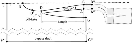
Figure 6.
Model 1 (CCA1) topology.
- (a)
- The axial extent of diffuser 1 (A–C) referred to as “Length”. This variable implicitly determines the position of the off-take along the strut. Low values of length correspond to flush off-takes and high values to total off-takes.
- (b)
- The “Angle” of the off-take (C–A) relative to the local slope of the strut (E–G). At a 0° angle the duct would locally be parallel to the strut surface.
- (c)
- The “Height” of the off-take which is explicitly defined by the distance C–D.
A set of different instances of model 1 for various values of the three input variables can be observed in Figure 7.
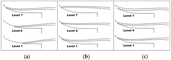
Figure 7.
Examples of different instances of model 1 variables. (a) Length; (b) Angle; (c) Height.
Figure 8 illustrates the control points and curves that constitute model 2. A robust method to design and parametrically control the shape of the manifold, typical for s-duct design, is the cubic Bezier curve equation, defined as:
where are the four control points of the Bezier curve and is the dimensionless length of the Bezier curve. Applying in two dimensions yields two Cartesian coordinates for each point and . Following this approach, the design of a single Bezier curve requires the definition of four points, which means that a total of thirty-two coordinates are required for the full definition of the manifold. Conveniently, many of these parameters can be eliminated using straightforward boundary relationships. To begin with, and , which are the start and end points of each Bezier curve, must be fixed in both the X and Y directions due to the condition that the s-duct must be connected to the upstream and downstream components. This only leaves the coordinates of points and to be defined for each curve. To ensure a smooth blend of the Bezier curves with the upstream and downstream components, the Y coordinates of points and are defined as a function of their X coordinate and the slope of the neighbouring curve to each point. With these simplifications, complete control of a Bezier curve can be provided solely by the axial coordinate of the two intermediate points and and a set of thirty-two variables defining the manifold has now been reduced to just eight. In this way, the value of a control point expresses the axial distance from start (upstream) to end (downstream) of a Bezier curve. Selected (optimal) solutions of s-duct 1 and s-duct 2 are later combined to construct the subsequent optimal manifold designs. Subscripts and superscripts of the Bezier control points follow the notation of Figure 8.
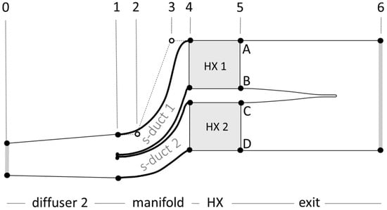
Figure 8.
Model 2 (CCA2) topology.
Details of all curve entities of the two models are summarised on Table 1. Furthermore, Table 2 presents a summary of all components of model 1 and model 2, the associated design variable description, and the selected evaluation methods.

Table 1.
Model 1 and model 2 setup details.
Table 2.
Complete parametric model summary and factorial design input.
3.2. Design Objectives
The criteria that best describe the “quality” of an aerodynamic system may vary from one problem to the next. However, a parameter of paramount importance in most aerodynamic systems is total pressure loss. More specifically high-pressure loss may affect the flow capacity of the cooling system and extensively it can impact the overall engine’s efficiency. It is therefore important that total pressure loss is considered as an objective in the current system. In this way, spatially averaged values of total and static pressure at a reference section are derived using the mass-weighted technique described by Klein [17]:
subsequently, the first design objective is a mass-weighted total pressure loss coefficient defined as:
where index “s” corresponds to the captured stream-tube and index “T” corresponds to the target zone. The captured stream-tube condition is defined at an adequate distance upstream of the bifurcation strut and is not significantly affected by changes in the input variables of model 1. There are four different regions where a loss coefficient is evaluated in this work including the loss in the bypass duct (), the loss in the CCA duct of model-1 () and the loss in the CCA duct of model-2 (). Note that the loss across the HX () is incorporated in .
Another important parameter in cooling systems is the uniformity of the flow delivered to the HX. Specifically, mal-distributed feeds can significantly affect the aerothermal performance of a HX, see Kwan et al. [18] and Raul et al. [19]. For this reason, the second design objective of this work is defined as the area-weighted non-uniformity index of the velocity magnitude at the HX inlet face (the target zone), calculated as:
where is the facet index of a surface with n facets, and is the area weighted average of the velocity at the HX inlet. A perfectly uniform flow would have a value of . This parameter was used by Spanelis et al. [9] on a single objective optimisation of a dual s-duct configuration similar to the one tested here.
A common issue in highly loaded duct systems is flow separation and recirculation, not only because of the high associative pressure losses, but also due to induced vibrations which can become a mechanical concern. In general, flow separation gives rise to an increased production of turbulence kinetic energy at the shear layer of the separation bubble (see for instance the highly resolved Large Eddy Simulation data reported by Luiz Schiavo [20] who investigated the turbulence kinetic energy budgets in turbulent channel flows with pressure gradients and separation). An increase in the production of turbulence kinetic energy is a source of total pressure loss, hence, in most duct systems minimising the total pressure loss coefficient would be sufficient to minimise or, if possible, to eliminate flow separation. However, as it will be shown later in this paper, there is an additional source of total pressure loss that takes place at the frontal face of the heat exchanger which conflicts with the upstream duct losses. This means that minimising the total pressure loss coefficient in the current problem does not guarantee minimization of the duct losses and subsequent flow separation. To resolve this issue, a third design objective is introduced that explicitly evaluates the turbulent activity in the delivery duct. More specifically, the kinetic energy ratio is defined as the mass-weighted volume integral of turbulence kinetic energy (TKE) in the delivery duct normalized by the mean kinetic energy (MKE) of the bulk flow in the same region. This is:
where n is the number of cells in the examined fluid volume and , , and are the cell values for turbulence kinetic energy per unit mass, density, volume and dynamic pressure respectively. To better understand the meaning of the kinetic energy ratio , assume a finite fluid volume with uniform velocity and turbulence intensity, (U) and (I), respectively. The turbulence kinetic energy per unit mass in this fluid volume can be expressed as . In the same region the bulk flow kinetic energy per unit mass can be expressed as . Combining these two equations in Equation (6) the kinetic energy ratio relates to turbulence intensity as . For instance, a value of is representative of an average turbulence intensity in the examined fluid volume of I=10%. Furthermore, it is important that is weighted appropriately so that it is insensitive to small variations in the turbulence kinetic energy in the flow-field but still, maintains sensitivity to radical changes, such as a flow separation/recirculation where turbulence intensity generally increases by a greater factor.
3.3. Multi-Objective Function
An “optimised” solution can be achieved by minimising one or more of the objective functions presented above. However, an attempt to improve a design objective may lead to the degradation of another which constitutes a non-trivial optimisation problem. A workaround is the establishment of a global function, the minimum value of which corresponds to the “best” compromise between the conflicting objectives, i.e., a scalarisation method. A multi-objective function is proposed, which can be classified as a weighted global criterion method, and is defined by:
More specifically, function calculates the normalised Euclidean distance in the criterion space , where is the value of a given design objective and is its utopia point, and subsequently applies a scaling and a weighting operation. Particularly, is the vector of scaling factors and consists of two components. The first component of the denominator, , represents the highest acceptable (critical) value for a given design-objective and the second component, , represents its lowest (ideal) value, i.e., the utopia point. Both these constants must be defined by the decision maker for each design objective and the range between these two values is referred to as the “acceptable design range”. In general, the utopia point is unattainable, and depending on the nature of the given design objective it may be difficult to evaluate. On a factorial design, however, the complete data sample is acquired before it is analysed, hence the minimum observed value of each design objective is known in advance. Therefore, the utopia point is approximated based on the minimum observation as:
where represents fixed contributions to a design objective. There are three such occurrences in the current study including:
- (a)
- The contribution of the bifurcation strut blockage to the bypass duct loss in model 1.
- (b)
- The HX loss in the overall CCA duct loss of model 2.
- (c)
- The turbulence intensity at the inlet of model 2 in the kinetic energy ratio.
If no constant contributions can be identified, i.e., , Equation (8) reduces to:
The minimum observation of a design objective, , may approach but it can never equal the utopia point , i.e., . In this study, an estimated value of is selected, meaning that the utopia points are approximated at a level 20% lower than the minimum observations. Since the utopia point is always lower than the value of the objective function, the value of must always be positive. Additionally, on a “bad” design, the objective function could exceed the critical value, , hence, does not have an upper limit. Finally, is the vector of weighting factors evaluated by the decision maker. The relative values of these weights determine the influence of each design-objective in the multi-objective function. It is noteworthy that the vector of scaling factors, , as well as the one of weighting factors, , in Equation (7) are both means of weighting the design objectives. The former is explicitly defined by the physical extremities of the problem and is therefore a more robust way to weight the outputs. However, the later can be very useful when the decision maker wishes to assign different levels of importance to the outputs. A review of multi-objective optimisation methods for engineering can be found at Marler and Arora [21].
3.4. Numerical Simulation Setup
The commercial CFD platform ANSYS Fluent was employed and the numerical simulations have been executed on a Linux machine using four CPU cores per run. This study has not considered compressibility effects; hence, a pressure-based solver was employed. Pressure-velocity coupling has been implemented via the SIMPLE algorithm (see Versteeg and Malalasekera [22]). Turbulence closure was achieved using the Reynolds stress model (RSM). Walker et al. [23,24] showed that this higher order model is required to capture the effects of curvature in an annular s-duct. A second order upwind scheme was applied for spatial discretization of momentum, turbulence kinetic energy, turbulence dissipation rate, and Reynolds stresses. Spatial discretization of pressure was implemented with the PREssure STaggering Option (PRESTO!) scheme in model 2 simulations due to lack of compatibility of the second order scheme with the porous media approach employed by Fluent.
A grid convergence study was conducted for two different geometries taken from model 1. Six different mesh densities in the range 3.0 × 10⁴ ≤ N ≤ 2.5 × 10⁵ were evaluated based on the total pressure loss coefficient of the CCA duct in model 1, . Results of this study are presented in Figure 9 which shows that the total pressure loss changes significantly with mesh density at 2 × 10⁴, but the solution is effectively invariable at mesh density of 5 × 10⁴ or higher and this is therefore the chosen density for the current work. At this mesh density, the off-take mouth is resolved by 20–25 cells depending on the off-take height and the HX inlet face is resolved by 55 cells. Boundary layer inflation is applied on wall boundaries with a growth rate of 1.2. The resulted non-dimensional wall distance varies as , which is compatible with the selected near-wall modelling approach, i.e., standard wall functions. Note that model 1 and model 2 mesh sizes are similar in this work and the details mentioned above apply to both models. Examples of meshing for the two models are shown in Figure 10 and Figure 11 respectively.
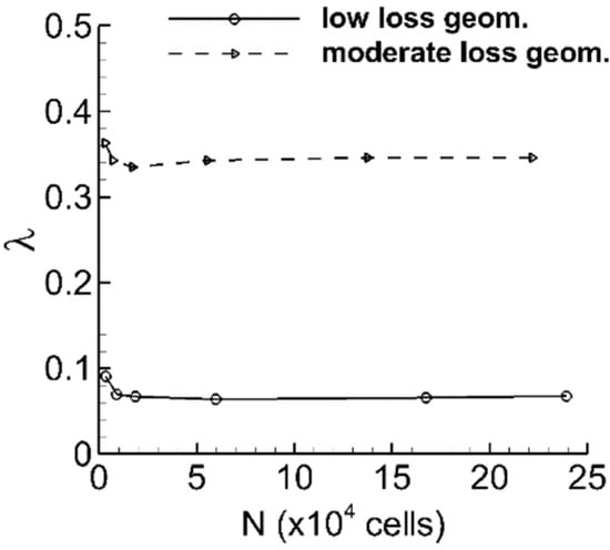
Figure 9.
Model 1 grid convergence study.
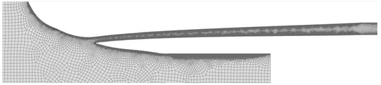
Figure 10.
Example of Model 1 meshing.
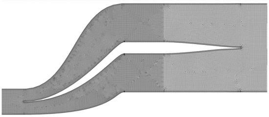
Figure 11.
Example of Model 2 meshing.
Furthermore, the inlet boundary of model 1 is fed by a profile of fan OGV exit velocity data representative of a commercial turbo-fan engine. Note that this is not explicitly presented here for reasons of confidentiality, but its effect to the bypass duct flow field can be observed in the velocity contour plots of Section 4. The mass flow ratio between the two outflow boundaries of model 1 is fixed at which is the requirement to feed two heat exchangers at max take-off engine conditions as calculated in the corresponding HX study by Ha et al. [25]. Velocity and turbulence data at the target zone of the optimal solution of model 1 are fed into model 2. More specifically, the x and y-velocity components, the turbulence kinetic energy, its dissipation rate and the full set of Reynolds stresses , , and , are interpolated at the inlet boundary of model 2. For further details about boundary type selection, refer to Table 1.
Finally, HX blockage is modelled via porous media through the application of a uniform inertial porous resistance of in all three directions. Here, the dynamic head of a perfectly uniform flow at the HX inlet is used in the evaluation of the loss coefficient, i.e., . This loss coefficient was calculated from the data of Ha et al. [25] in line with a requirement for a 3.25% pressure drop ( across the HX with respect to the bypass duct condition of a commercial turbo-fan engine at max take-off conditions. Turbulence in the porous medium is solved using the standard conservation equations and microscopic effects to turbulence kinetic energy are not accounted for (see Pedras et al. [26]).
4. Model 1 Results and Discussion
4.1. DoE 1 Data Sampling and Objective Function Conditioning
The first step in the execution of a factorial design is the selection of the sampling method. Here a domain-based approach is employed, aiming to uniformly distribute the sampling points in the design space. A subset of the sample, including the extreme and mid-values for each of the three input variables, is illustrated in Figure 7. The actual variable ranges are available on Table 2.
The results of DoE 1 are initially plotted in a three-dimensional criterion space defined by the three selected design-objectives. In this type of plot, each individual level of the factorial design assigns a single point, i.e., the points that appear in Figure 12 are the imprints of the three-dimensional cloud projected on the three mutually perpendicular planes. More specifically, the three two-dimensional criterion spaces that result this decomposition are shown in Figure 12 in sub-figures:
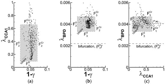
Figure 12.
DoE 1 results—Projected 3D criterion space into three individual 2D components (a–c).
- (a)
- total pressure loss in the delivery duct against diffuser 1 exit non-uniformity,
- (b)
- total pressure loss in the bypass duct against diffuser 1 exit non-uniformity and
- (c)
- total pressure loss in the delivery duct against the one in the bypass duct.
In Figure 12a,b it can be observed that there is no design point for which both objectives are simultaneously minimised. Instead, a frontier of optimal solutions tends to form at the bottom left of each of these two plots, a.k.a. a Pareto frontier (see Pareto [27]). On the contrary, the two objectives of Figure 12c exert a different behaviour. More specifically, it is indicated that the losses of the CCA duct and the ones of the bypass duct are minimised simultaneously, which constitutes a trivial multi-objective optimisation problem. It should, however, be born in mind that by nature the current factorial design methodology cannot guarantee an absolute optimal solution nor an actual Pareto frontier; this would effectively require an infinite number of DoE training points. There is a wide range of intelligent optimisation techniques, capable to optimise nonlinear multimodal functions, such as genetic algorithms, tabu search, simulated annealing and neural networks, see for instance the recent review of Pham and Karaboga [28]. However, this endeavour is beyond the scope of the current work which, as part of a preliminary design exploration, primarily aims to characterise the design space without necessarily finding the true optimal solution.
Additional information that can be drawn by Figure 12 is the effectiveness of the selected parametrisation approach. In an optimisation study it is preferable that the training points appear at an increased concertation in the direction of the utopia point. In this paper the design variables (inputs) of the DoE study are distributed uniformly in the design space. The output data distribution in criterion space indicates the effectiveness of both the input variable definition and to the selected input variable ranges. In this respect Figure 12 indicates that the parametrisation of DoE 1 is effective in the exploration of the by-pass duct loss and the CCA duct loss but it appears that the density of the sampling points near the optimality of non-uniformity is low. To better understand this behaviour the results must be viewed in design variable space which is discussed in the next section.
The highlighted (grey) region in the plots of Figure 12 is the projection of the three-dimensional window upon which the objective functions are scaled. The boundaries of this window are defined by the values of and applicable in Equation (7). More specifically, in this example the critical value above which the pressure loss in model 1 ( is unacceptable has been empirically set to . This value is strongly application-specific; here it was set based on the available pressure differential (in the engine) which drives the bleed system. Furthermore, the critical value for non-uniformity (1 − has been set to 8 after a qualitative examination of different non-uniformity values on a representative selection of velocity profiles as shown in Figure 13. A critical value for the bypass duct loss ( can be estimated based on a fan equivalent polytropic efficiency of the bypass duct. More specifically, as shown by Kyprianidis [29] (Figure 14) for every 1% increase of the bypass duct pressure loss () on a fan at moderate pressure ratio (i.e., ) the equivalent polytropic efficiency drops by approximately 2%. The current study attempts to limit the equivalent polytropic efficiency drop induced by the off-take at . Based on the plot of Figure 14 this corresponds to a critical increase in by-pass duct loss of order . On a typical turbofan engine in max take-off conditions this coefficient can be expressed in terms of inlet dynamic head as . Further to the off-take spillage loss, inherent in the bypass duct region is part of the aerodynamic loss of the bifurcation geometry itself. This has been quantified here via a pre-cursor simulation of the same bypass duct section but without an off-take and it was predicted as . This value can be considered as a constant offset of the critical value, i.e., . For the same reason this value also appears as a constant offset in the evaluation of the utopia point in Equation (8), i.e., . The utopia points of the other two objectives do not involve any known fixed contributions and are therefore calculated from Equation (9). A summary of the scaling parameters of DoE 1 is available in Table 3.
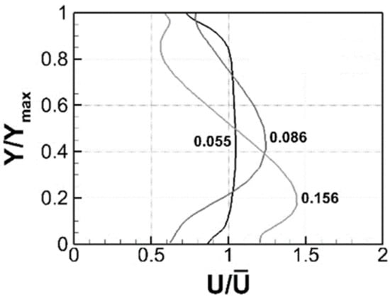
Figure 13.
Non-dimensional velocity profiles at the exit of diffuser 1 corresponding to a range of non-uniformities (1 − γ).
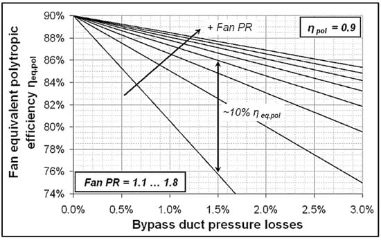
Figure 14.
Effect of fan tip pressure ratio and bypass duct pressure losses on fan equivalent polytropic efficiency, (from Kyprianidis [29]).
Table 3.
Scaling parameters for DoE 1.
4.2. DoE 1 System Response Analysis and Optimisation
DoE 1 results are illustrated in Figure 15 on a design variable space representation. For a cubic factorial design, the subsequent design space is three-dimensional. For simplicity the three principal axes of this space are labelled by the level number (1–7) of a variable instead of its actual value. The latter can be computed from the input data available in Table 2 with “min” corresponding to level 1 and “max” to level 7. Data are plotted on a selection of planes in this volume. More specifically, Figure 15a–d illustrates data on four intermediate planes of constant “height”. Each plot also includes an iso-surface of the design objective at a slightly higher value than the observed minimum. This iso-surface encloses a broader region of optimality. It is observed in Figure 15a that by increasing the length of diffuser 1 the cooling system experiences a reduction in delivery duct loss. The direct cause for this observation is the increase in the non-dimensional length of the diffuser as shown in the loading chart of Figure 16. The observed trend is dominant in the plot, i.e., there is a low level of interaction with the other two input variables (off-take angle and height). Such a strong behaviour is also attributed to the following conditions:
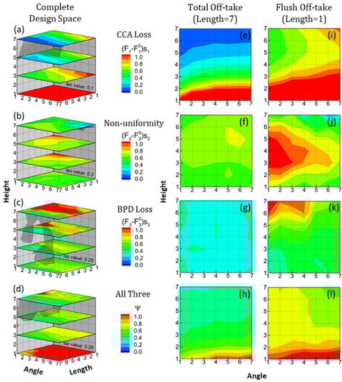
Figure 15.
Model 1 (DoE 1) system responses. Full design variable space (a–d), total offtakes (e–h), and flush offtakes (i–l).
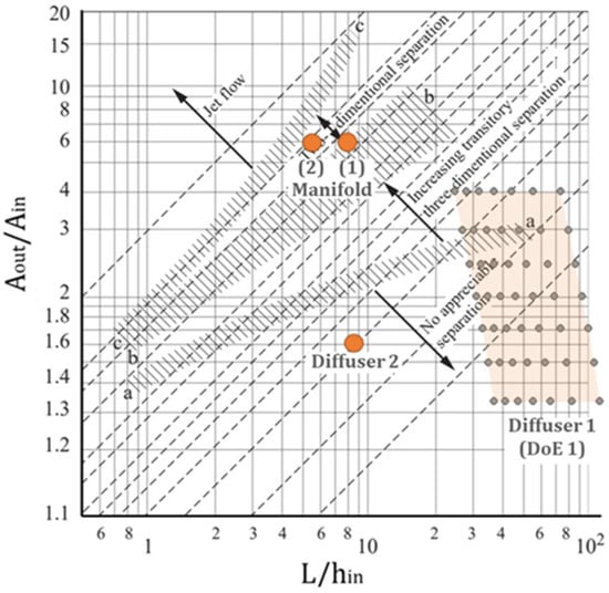
Figure 16.
Flow regimes for plane-walled, single-plane expansion diffusers [30].
- (a)
- There is a positive velocity gradient in the streamwise direction due to the strut curvature, i.e., the velocity near the leading edge is lower. Therefore, the pre-diffusion requirement of the captured stream-tube is reduced near the leading edge.
- (b)
- At the leading edge of the strut the off-take can fully exploit the dynamic pressure of the bypass stream, a general advantage of total off-takes over flush off-takes.
It is also observed that the losses in the delivery duct are inversely proportional to the off-take height. The observed output remains acceptable between planes 7 and 3, but near plane 1, it reaches prohibitively high levels, i.e., (red colour). This can be explained by the increasing flow speed for a decreasing off-take throat area. The flow velocity at the off-take throat is inversely proportional to its height (i.e., ) and the pressure loss is proportional to the square of the velocity (). Accordingly, the pressure loss is inversely proportional to the cube of the off-take height ().
Figure 15b indicates that the non-uniformity of the velocity profile at the exit of diffuser 1, for most of the design space is maintained at or of the acceptable range. This corresponds to which according to Figure 13 translates to highly uniform velocity profiles. Nonetheless, there is a region at low length, low off-take angle and intermediate off-take height, where non-uniformity increases beyond the acceptable limit, i.e., , which translates to . There is a narrow region of optimality for this design objective at low length (flush off-take), high off-take angle and large off-take height (open throat). This is a highly loaded off-take design as is well reflected by the increased losses of the captured flow in Figure 15a. A representative design from that region is illustrated in Figure 17 which shows that the increased CCA duct loss is caused by a separated off-take. The long duct section between the off-take and the target zone allows for the flow to reattach, while the convoluted flow path created by this separation coincidentally leads to a symmetric velocity profile near the target zone. The narrowness of this optimal region in the design space is product of this unstable flowfield and hence is a non-attractive option in a subsequent design selection.
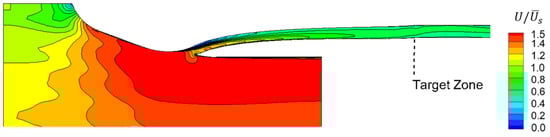
Figure 17.
Design of optimal non-uniformity in DoE 1, a1b6c7.
Furthermore, the effect of the three input variables to the bypass duct loss is illustrated in Figure 15c. The plot indicates that both a flush off-take and a total off-take may offer design options with minimal effect to the bypass duct flow (recall that one of the main reasons for the use of flash off-takes in the bypass duct of commercial turbofan engines is to protect the bypass duct flow from aerodynamic losses). Figure 15g and k suggest that, in a bifurcation installation a submerged off-take near the leading edge (i.e., a total off-take) may in fact impact the bypass duct even less than a flash off-take. Even more encouraging in the selection of a total off-take is the lack of observed interactions with the other two input variables, i.e., the off-take’s angle and height as shown Figure 15g. The robust behaviour of total off-takes is also demonstrated by a considerably flat distribution of non-uniformity across the angle-height design space (Figure 15f).
An optimal off-take design can now be selected from DoE 1. This is achieved via the multi-objective function, , as defined by Equation (7). The vector of scaling factors is constructed from the values of Table 3 while the vector of weighting factors is set to (i.e., equal significance between all three design objectives). The resulted contours are illustrated in Figure 15d,h,l. Red colour, i.e., indicates regions of low interest, where one or more of the objective functions exceed their critical value, i.e., , and green-blue colour indicates regions of increased interest, where the multi-objective function tends to minimise. The iso-surface of highlights the existence of a minimal value plateau at maximised length which confirms earlier indications of the superiority of total off-takes compared to flush off-takes. This plateau can be better observed in the contours of in Figure 15h.
Table 4 presents a summary of the input variable settings and the corresponding objective function values (output) for the three single-objective optimisations as well as the three-objective optimisation. The design with the minimum value of the multi-objective function is length = 7, angle = 1 and height = 7, or simply design “a7b1c7”. This geometry incurs a CCA duct loss of = 0.145, which can be expressed as in a scaled representation, or else of the acceptable output range. The non-uniformity of the selected optimal solution is and corresponds to a value of of the acceptable output range. The reason why the scaled value of non-uniformity of the selected design is relatively high is the existence of a group of aerodynamically unstable designs of low uniformity in the family of the one shown in Figure 17. The imprints of such designs can be distinctly observed in the criterion space of Figure 12a,b where a very low number of design points spreads through an extremely low non-uniformity region, i.e., . Lastly, the value of the bypass duct loss coefficient of the optimal geometry is = 0.00377 corresponding to 32% of the acceptable output range. The reason for this relatively high scaled value is that the constant offset of the bypass duct loss, i.e., , is relatively small compared to the minimum observation , i.e., . Nevertheless, this is only higher than the minimum observation as shown on Table 4.
Table 4.
Characteristics of the optimal geometries (inputs and outputs).
Figure 18 illustrates contours of normalised velocity magnitude and total pressure on the selected optimal geometry as well as a plot of the profile of velocity magnitude at the target zone. This profile, alongside the detailed description of turbulence, including the Reynolds stresses for the RSM model, are fed at the inlet boundary of model 2 to support DoE 2 and DoE 3 that follow.
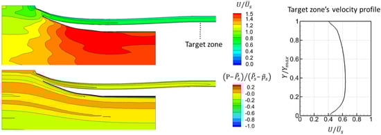
Figure 18.
Selected design of DoE 1, a7b1c7.
Figure 19 shows that for a broad range in the design space near the optimal region (low to moderate loss geometries) the flow profile delivered at the exit of diffuser 1 is virtually unchanged. Significant changes in the profile are observed in regions of high loss which can be understood by the mechanisms described in Figure 17. Such designs are of low value, hence, it can be claimed that the presented profile is representative of model 1 and indicates that fractionalisation of the problem to model 1 and model 2 should have a small effect to the outcome of this optimisation.
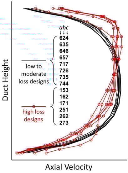
Figure 19.
Relative variation of the axial velocity profile at diffuser 1 exit in DoE 1.
5. Model 2 Results and Discussion
5.1. DoE 2 and DoE 3 Data Sampling and Objective Function Conditioning
As mentioned in the introduction, model 2 is a variation of the s-duct that was previously studied by Spanelis et al. [9]. In their work they mentioned that the duct losses are insignificant compared to the HX loss and accordingly they based their optimisation on the uniformity criterion alone. However, the present work considers a different parametrisation method which allows for even higher concentration of the aerodynamic loading near the HX, via an aggressive manifold. The mission of this aggressive manifold is to diffuse the flow at an area ratio of within a non-dimensional duct length of for s-duct 1 and for s-duct 2. According to the loading chart of Figure 16 both these s-ducts are severely loaded and would strongly separate were it not for the beneficial upstream influence of the HX.
Below it will be shown that this separation can in fact be avoided even in this extreme loading scenario, however, this is only achievable at the cost of an increased aerodynamic loss. For this reason, the pressure loss can no longer be omitted but it becomes an essential design objective.
To better understand the physical importance of the selected parametrisation method and subsequent selection of the design objectives, Figure 20 presents an aerodynamic comparison of two extreme manifold designs. Example A (left) is representative of a uniform loading distribution in the manifold and Example B (right) represents geometries that concentrate the loading at the exit, i.e., the front face of the HX. The figure shows contours of velocity , turbulence kinetic energy , production of k (  ) and total pressure , all normalised by suitable reference values to facilitate the comparison.
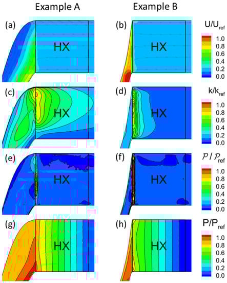
Figure 20.
Aerodynamic comparison of two extreme manifold designs in terms of velocity (a,b), TKE (c,d), production of TKE (e,f), and total pressure (g,h).
It can be observed that Example A is not an ideal approach and as suggested by the loading chart of Figure 16 a large flow separation forms in the s-duct. This separation is reflected on both the contours and streamlines of velocity magnitude of Figure 20a as well as the contours of turbulence kinetic energy of Figure 20c. Note that the latter increases considerably along the mixing layer of the separation wake of Example A. On the other hand, the flow in Example B remains attached throughout the s-duct as there is no significant cross-sectional area variation. This leaves almost all the diffusion and turning to take place within an extremely short distance immediately in the front of the HX. Nonetheless, this task is made possible due to the high blockage imposed by the HX, but as indicated by Figure 20f this highly concentrated loading brings about a large increase in the local shear stress, which is the source of an increased production of turbulence kinetic energy (Figure 20d) and consequently of an increase in total pressure loss (Figure 20h), hereinafter referred to as “HX entry loss”. While most of this loss takes place inside the HX, a significant proportion of it occurs inside the manifold (see Figure 21).
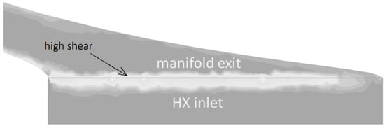
Figure 21.
Extreme production of turbulence kinetic energy around the manifold-HX interface.
The dominant loss in the current system takes place at the core of the HX and is referred to as “HX core loss”. Nonetheless, the HX entry loss may grow significantly, even to a comparable level to the HX core loss depending on the specific values of the input variables.
With the above in mind, the evaluation of the pressure loss of model 2 is not implemented directly at the target zone, which is at the HX inlet, but the evaluation is transferred at the HX exit plane which ensures that the HX entry loss is fully accounted for. More specifically, the total pressure loss coefficient in model 2 (DoE 2 and DoE 3) is calculated as:
Furthermore, flow separation and recirculation are common threats in duct systems, not only because they contribute strongly to the total pressure loss, but also due to vibration, noise and component fatigue that it may also lead to. Conversely, reduction of this type of loss in the current system, hereafter referred to as “delivery duct loss”, is predominantly achievable at the expense of an increased HX entry loss. As shown above the delivery duct loss and the HX entry loss are in strong conflict with one another; therefore, minimising their sum does not necessarily guarantee the minimisation of both individual contributions. Consequently, the pressure loss coefficient of Equation (10) is not suitable to indicate flow separation in the manifold. For this reason, the kinetic energy ratio of Equation (6) is employed as a separate design objective. This parameter indicates variations in the overall turbulence level in the delivery duct, therefore, it can identify the presence of significant flow separation. In summary, the design exploration of model 2 considers the following objectives:
- (1)
- Total pressure loss across the system.
- (2)
- Non-uniformity of the velocity magnitude at the inlet of the HX.
- (3)
- Kinetic energy ratio in the delivery duct.
Additionally, the multi-objective function of Equation (7) is evaluated based on the vector of scaling factors available on Table 5. More specifically, the utopia point for non-uniformity, , and turbulence kinetic energy, , are calculated based on the observed minima from Equation (9). On the other hand, the HX loss coefficient is a fixed boundary condition and given that the HX core flow is highly uniform in the explored design space, the HX core loss is not likely to vary significantly. In this way, the utopia point for the total pressure loss, is calculated from equation (8) by setting the HX loss as a fixed contribution, i.e., . Furthermore, the critical value for total pressure loss has been set to for both DoE 2 and DoE 3 ensuring that the HX core loss will remain as the dominant contribution in the acceptable design range. Moreover, the critical values of non-uniformity and kinetic energy ratio are empirically set to 0.2 and 0.1 respectively based on the observed ranges of DoE 2 and DoE 3. A complete summary of the scaling coefficients of DoE 2 and DoE 3 is available on Table 5.
Table 5.
Scaling parameters for DoE 2 and DoE 3.
Finally, Figure 22 and Figure 23 illustrate the results of DoE 2 and DoE 3, respectively, on a projected criterion space using a similar format to that of Figure 12. It can be observed that the training points are well distributed in the criterion space except for the non-uniformity which presents a significant drop in density in the direction of the utopia point. Furthermore, the ranges of the observed output criteria of DoE 2 are relatively narrow which indicates weak response level to the input variables compared to DoE 3. This is attributed to the relatively low vertical to axial displacement ratio of s-duct 2 (∆𝑌/∆𝛸 = 0.77) compared to s-duct 1 (∆𝑌/∆𝛸 = 1.63). More specifically, according to the current parametrisation of the Bezier curves (i.e., varying only the x-coordinates of the intermediate control points) a curve with elevation ∆𝑌/∆𝛸 = 0 would be unresponsive to the input variables. However, as the value of ∆𝑌/∆𝛸 increases the interactions between the two curves also increase, leading to an increase in the degrees of freedom of the aerodynamic definition of the duct geometry.
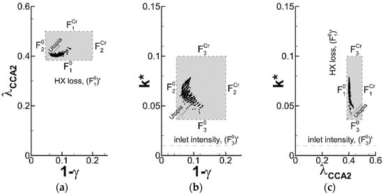
Figure 22.
DoE 2 results—Projected 3D criterion space into three individual 2D components (a–c).
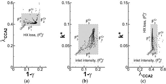
Figure 23.
DoE 3 results—Projected 3D criterion space into three individual 2D components (a–c).
To construct a more efficient parametric model and overcome the issues mentioned above, one must first understand which regions of the explored design space offer improved aerodynamic properties. The following analysis is dedicated to this goal.
5.2. DoE 2 and DoE 3 System Response Analysis
Contour plots of the scaled objective functions in the design-variable spaces of DoE 2 and DoE 3 are illustrated in Figure 24 following the same format as previously described for Figure 15a–d. It is observed that all three objective functions conflict with one another and each design objective is minimised at a different region. The loss coefficient minimises at coordinates = 1, = 1 and = 4 in DoE 2. For simplicity, this design is referred to as “a1b1c4” (Figure 15a). Similarly, the minimum loss coefficient in DoE 3 is observed at design “a5b5c6” (Figure 15b). Furthermore, the non-uniformity minimises near the opposite side of the cubic volume, i.e., design a7b5c6 in DoE 2 (Figure 15c) and design a6b7c6 in DoE 3 (Figure 15d). Additionally, the kinetic energy ratio minimises at design a4b7c1 in DoE 2 (Figure 15e) and design a5b7c1 in DoE 3 (Figure 15f). Finally, the three design objectives are combined into a multi-objective function which minimises at design a4b7c3 in DoE 2 (Figure 15g) and a5b7c5 in DoE 3 (Figure 15h).
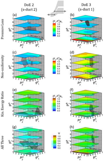
Figure 24.
Model 2 (DoE 2 and DoE 3) system responses in all design objectives. Plotted outputs include: Pressure loss (a,b), non uniformity (c,d), kinetic energy ratio (e,f), and the multi-objective function (g,h).
Note that there are certain regions in both the DoE 2 and DoE 3 design spaces that have been blanked out. The reason is that CFD data are unavailable at those regions due to some failure in the geometry/mesh generation or the numerical simulation. The most typical reason for failure of an instance execution is that the input variables lead to an unphysical shape such as a self-intersecting geometry. A less frequent scenario is when the geometry and mesh were in fact successfully generated but the numerical simulation did not achieve convergence. Usually, such designs are of low aerodynamic interest and failing to execute them is in fact beneficial as it saves computational resources.
The first component in model 2 is diffuser 2. While diffuser 2 is an inherent part of all simulated instances of DoE 2 and DoE 3, the actual geometry definition of this component does not vary in this study. The inlet height of model 2 is defined as the exit height of model 1 and the exit height of diffuser 2 (or manifold inlet) has been pre-fixed using input from the loading chart of Figure 16 corresponding to a stable diffuser. The numerical predictions of a single instance in DoE 2 and DoE 3 are presented in Figure 25. More specifically, Figure 25a,b and illustrate contours of normalised total pressure and normalised velocity magnitude respectively. It can be observed that the high-quality flow imported from model 1, in conjunction with the moderate loading of diffuser 2, has led to flow without separation within the diffuser. Nonetheless, the momentum thickness presented to the manifold is increased in both walls and it is part of the mission of DoE 2 and DoE 3 to optimise the manifold geometry to negotiate this condition.
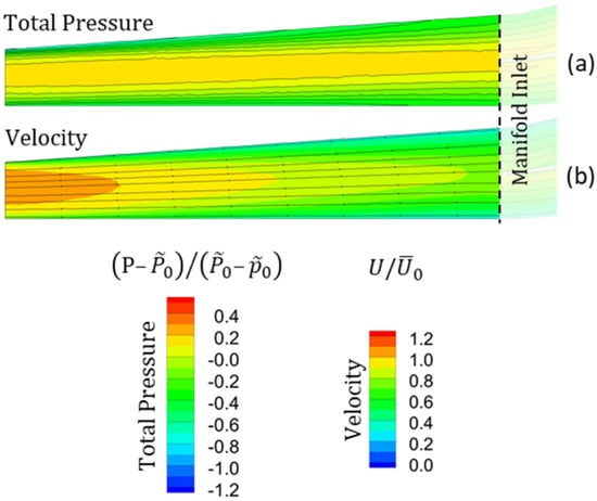
Figure 25.
Diffuser 2 CFD prediction—Contours of normalised total pressure (a) and normalised velocity magnitude (b).
A comprehensive understanding of the aerodynamic behaviour of the manifold in the explored design space requires that a representative sub-range of designs from DoE 2 and DoE 3 are individually characterised. A sub-range is selected so that all analysed designs are aerodynamically optimal, based on one or more of the selected design objectives. More specifically, a design objective, , can be excluded from the multi-objective function by setting the respective weighting factor to (see Equation (7)). Conversely, the value of can be used so that a given design objective is considered. With this method all seven combinations of weighting have been considered in both DoE 2 and DoE 3. The fourteen individual optimal s-duct designs are then combined to create the seven corresponding instances of the complete manifold. Contours of normalised total pressure, velocity magnitude and kinetic energy ratio of the seven optimal manifold designs are illustrated in Figure 26 and Figure 27, corresponding to single objective and multi-objective optimisations respectively. Note that for consistency Figure 25, Figure 26 and Figure 27, share the same contour ranges. The manifold design that exhibits minimal aerodynamic losses is referred to as “-optimum”, the one that minimises the non-uniformity as “-optimum” and the one that minimises the kinetic energy ratio as “-optimum”. Similarly, the two-objective optimisations are referred to as “--optimum”, “λ--optimum” and “--optimum” respectively. Finally, the three-objective optimal design is referred to as “overall-optimum”, not to be confused with the true optimum, which, as explained above is unattainable with the present sampling method.
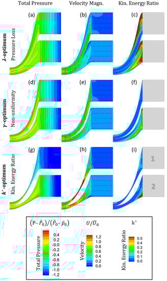
Figure 26.
Contours of normalised total pressure, velocity magnitude and cell based kinetic energy ratio on the three single-objective optimal solutions: λ-optimum (a–c), γ-optimum (d–f), and k*-optimum (g–i).
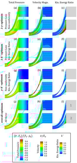
Figure 27.
Contours of normalised total pressure, velocity magnitude and cell based kinetic energy ratio on the multi-objective optimal solutions: λ-γ-optimum (a–c), λ-k*-optimum (d–f), γ-k*-optimum (g–i), and the overall optimum (j–l).
Table 6 presents the weighting coefficients as well as the values of the three input variables leading to each one of the seven optimal solutions. Recall that for simplicity the level number (1–7) is reported instead of the actual value of the input variables. Furthermore, Table 7 presents the scaled criteria of the seven optimal solutions.
Table 6.
Weighting and input variables for optimal designs of DoE 2 and DoE 3.
Table 7.
Optimal design outputs of DoE 2 and DoE 3.
5.3. DoE 2 and DoE 3 Single Objective Optima
In general, the numerical predictions presented in Figure 26 indicate that depending on the selected optimisation criteria the optimal aerodynamic shape of the manifold can vary significantly. More specifically, the first single-objective optimisation has minimised the pressure loss across the manifold. A typical method to achieve that in simple duct systems is by diffusing the flow early in the duct in order to reduce the average flow speed. However, in the current problem, loss minimisation has a rather more complex relationship to geometrical inputs than that of a simple diffuser due to the conflict between the delivery duct loss and the HX entry loss discussed above. The numerical predictions of the -optimum geometry (Figure 26a–c) indicate that it expands faster compared to the other two single objective optimal solutions (Figure 26d–i). However, it is evident from the contours of velocity and kinetic energy ratio (Figure 26b,c) that the flow of -optimum separates in both s-ducts. Therefore, as seen in Table 7, the -optimum has been achieved at the expense of high penalties in the other two objectives. These include a and increase in the kinetic energy ratio of s-duct 2 and s-duct 1 respectively and a 51% increase of the non-uniformity of s-duct 1. Note that these values are the differences from the overall-optimum geometry.
The second single objective optimisation has minimised the non-uniformity of the velocity profile delivered to the HX. As mentioned above, a -optimum can be the result of any combination of events that favours the formation of a uniform velocity profile at the target zone. Here the preferred duct shape for a -optimum design appears to be consistently at an increased angle of approach and of minimal diffusion in the manifold (see Figure 26d–f). This leads to an increased loading at the HX entry. Table 7 shows that this increased loading has a large impact to the HX entry loss which for s-duct 1 is higher than that of the overall-optimum. Furthermore, since no significant loading is applied by s-duct 1, there is no significant flow separation in it either. Consequently, the value of kinetic energy ratio is not affected significantly (i.e., it is only higher than the overall-optimum). As mentioned earlier, the lateral displacement of s-duct 1 (ΔY) is larger than that of s-duct 2 which reduces the degrees of freedom of the latter. This has limited the ability of s-duct 2 to form high approach angles to the HX and extensively its ability to limit the amount of diffusion practical upstream of the HX. Furthermore, as indicated by the contours of velocity in Figure 26e, the adverse pressure gradient which is the combined effect of duct’s diffusion and of the concave curvature of the inner wall of s-duct 2, has caused the flow to separate early. This separation has contributed to a considerable increase of the kinetic energy ratio in s-duct 2 which according to Table 7 is higher than that of the overall-optimum.
The third single objective optimisation has minimised the kinetic energy ratio of the manifold. Recall that the kinetic energy ratio expresses the proportionality of turbulence kinetic energy (TKE) to the mean kinetic energy (MKE) within a given fluid volume. Flow diffusion causes the mean flow velocity and extensively MKE to reduce. At the same time, flow diffusion promotes boundary layer thickening and possible flow separation, hence causes TKE to increase. The more upstream any of these events occurs, the larger the affected fluid volume, hence the higher the kinetic energy ratio. For this reason, a -optimum design favours narrow ducts with increased flow velocity and thin boundary layers. Regardless of the area distribution in the s-duct, the flow eventually must be diffused to the size of the HX. However, the higher the aerodynamic loading, the closer to the HX it must be applied in order to avoid a local flow separation in front of the HX. Again, for the same reason as mentioned above, s-duct 1 is more capable in obtaining a favourable shape than s-duct 2. More specifically, the contours of cell based kinetic energy ratio of Figure 26i show that although some flow separation is observed near the exit of s-duct 1, this is considerably smaller than the strong recirculation that has been formed at the exit of s-duct 2.
Expectedly, this recirculation has severely affected the non-uniformity of s-duct 2, i.e., it has increased by compared to the overall-optimum as shown on Table 7. On the other hand, the increased velocity in s-duct 1 has severely affected the system losses, which in fact have exceeded the acceptable limit () of DoE 3. Figure 26g illustrates the effect of this extreme loss to the total pressure field and Figure 26h its effects on the velocity field. The latter indicates that there is an imbalance in mass flow between s-duct 1 and s-duct 2. Given that model 2 has a single inlet and a single exit, the mass flow balance between s-duct 1 and s-duct 2 is determined by the individual system losses. However, since the HX loss is dominant in model 2, the mass flow imbalance between s-duct 1 and s-duct 2 is in general low, i.e., with minimal variations for for the majority of the design space, where is the mass flow rate at the inlet of model 2 and is the deviation of the actual mass flow from an ideal mass flow split. Exception to this is a narrow region in the design space of extremely imbalanced designs, such as the one of -optimum, where values of mass flow imbalance of up to are observed.
5.4. DoE 2 and DoE 3 Multi Objective Optima
The analysis above has highlighted the aerodynamic effects of the three individual objective functions and exposed the limitations of single objective optimisation in this problem which has led to the present multi-objective approach. Nonetheless, Figure 27a–i reveal that the same stands for all two-objective optimisations. More specifically, Figure 27a–c reveal that --optimum displays a good balance between pressure losses and uniformity, but it suffers from flow separation in both s-ducts. Notice the increased kinetic energy ratio region at the concave side of diffuser 2 (Figure 27c) which according to Table 7 contributes to a general increase of this parameter of compared to the overall-optimum. Moreover, --optimum (Figure 27d–f) is in fact a strong competitor of the overall-optimum in most respects. However, there is a small region of flow recirculation at the HX inlet of s-duct 2 visible on the contours of both the velocity and the kinetic energy ratio. Although this flow separation is too close to the duct exit to cause any significant increase of the kinetic energy ratio, it takes place exactly on the location where non-uniformity is evaluated. For this reason, the non-uniformity of --optimum is higher than the overall-optimum as shown in Table 7. Note that a flow recirculation near the HX could have catastrophic consequences in the real engine application as it would allow heat to accumulate at the front of the HX. The numerical predictions of the third two-objective optimisation, --optimum, are presented in Figure 27g–i. The main problem of this geometry is the excessive loss in s-duct 1 due to the extremely high blockage, like the -optimum above.
Finally, as shown in Table 7 the overall-optimum has relatively low values of all three design objectives. Furthermore, the contours of normalised total pressure in Figure 27j, show that the system is well balanced in the two HXs. Moreover, the contours of velocity magnitude in Figure 27k reveal that the flow in both s-ducts is highly uniform. However, the results of kinetic energy ratio in Figure 27l reveal a growing boundary layer at the concave wall of s-duct 2 near the HX, imposing an imminent danger for flow separation. This region has been challenging in all seven optimal solutions but clearly the overall-optimum alongside --optimum offer considerable improvements.
Two suggestions for further improvement of this issue are: (a) increase the amount of diffusion practical in diffuser 1 aiming to relieve the manifold and (b) install inlet guide vanes at the front of the HX to support the steep turning. Furthermore, the current results suggest pushing further the flow turning at HX inlet, i.e., beyond the limitations of the current parametrisation. Two alternative approaches would be: (i) to explicitly define the s-duct exit angle as a separate design variable and (ii) to increase the order of the Bezier curve from third to fourth in order to increase the degrees of freedom of the s-dust geometry. While these modifications require the addition of new variables, with the help of the present data the existing number of variables can be reduced. For instance, in the next design stage the design space can be narrowed down closer to one of the nominal designs shown in Figure 26 and Figure 27. For each of these nominal designs certain variables are ineffective, therefore, can be set as constants. However, the actual candidate to proceed to the next design stage depends on the current needs of the greater system, in this case this is the full CCA system which consists of other subsystems that evolve in parallel.
6. Conclusions
This paper presented a simple numerical methodology for the multi-objective design exploration and optimisation of aerodynamic systems in the conceptual/preliminary design stage. The method, which employs a fractional factorial design technique, is based on the simplification of the examined problem to its leading order aerodynamic characteristics. This allows for an increased sampling resolution that renders it suitable for the explicit evaluation of nonlinear interactions between widely explored input variables. The method was applied on a conceptual aero-engine duct system that involves an aerodynamic off-take on the large bifurcation strut of the bypass duct, followed by a complex delivery duct. The latter includes a manifold that feeds an array of low permeability heat exchangers. The analysis indicated that optimal geometries may vary significantly depending on the selected quality criteria and motivated the construction of a global criterion based on the scalarisation technique which subsequently facilitated a robust multi-objective assessment. The results showed that, for the chosen design objectives, a submerged off-take at the leading edge of the strut, which effectively acts as a total off-take, is overall a better design choice compared to a flush off-take on the side walls of the strut. An aerodynamic comparison between single and multi-objective optimal design solutions of the heat exchanger manifold highlighted the weaknesses of each individual single objective optimisation and demonstrated the ability of the multi-objective approach to improve them and to indicate a family of trade-off solutions. The presented results are only a small sample of what can be inexpensively acquired during the late conceptual/early preliminary design stage, by progressively refining the design variables (inputs) and the multiple design objectives (outputs). However, the presented methodology has a broader applicability and can be used to develop efficient, problem-specific, parametric models, narrow down design spaces, facilitate nominal design selection and build efficient surrogate models to be used on more expensive numerical or even experimental campaigns at subsequent, more mature design stages.
Author Contributions
Conceptualization, A.S.; Data curation, A.S.; Formal analysis, A.S.; Funding acquisition, A.D.W.; Investigation, A.S. and A.D.W.; Methodology, A.S.; Project administration, A.D.W.; Resources, A.D.W.; Software, A.S.; Supervision, A.D.W.; Validation, A.S.; Visualization, A.S.; Writing—original draft, A.S. and A.D.W.; Writing—review & editing, A.S. and A.D.W. All authors have read and agreed to the published version of the manuscript.
Funding
This research received no external funding.
Conflicts of Interest
The authors declare no conflict of interest.
Abbreviations
| BPD | Bypass duct |
| CCA | Cooled Cooling Air |
| DoE | Design of Experiments |
| HP | High Pressure |
| HX | Heat Exchanger |
| LP | Low Pressure |
| MKE | Mean Flow Kinetic Energy |
| OGV | Outlet Guide Vane |
| PR | Fan Pressure Ratio |
| TKE | Turbulence kinetic energy |
| Symbols | |
| Area | |
| Vector of objective functions | |
| Utopia point | |
| ( | Fixed offset of utopia point |
| Vector of critical values | |
| Vector of observed minima | |
| Heat exchanger height, used as reference length | |
| Turbulence kinetic energy | |
| Kinetic energy ratio | |
| Total pressure | |
| Vector of Bezier curve control points | |
| Production of turbulence kinetic energy | |
| Static pressure | |
| Dynamic pressure | |
| Vector of scaling coefficients | |
| Velocity magnitude | |
| Volume | |
| Vector of weighting coefficients | |
| γ | Uniformity index of velocity |
| λ | Total pressure loss coefficient |
| Density | |
| Multi-objective function | |
| Area-weighted averaging operator | |
| Mass-weighted averaging operator | |
| Indices | |
| Captured stream-tube (at CFD inlet plane) | |
| Target zone | |
| Grid cell ID and objective function ID |
References
- Walker, A.D.; Koli, B.R.; Spanelis, A.; Beecroft, P. Aerodynamic design of a cooled cooling air system for an aero gas turbine. In Proceedings of the 23rd International Symposium on Air Breathing Engines (ISABE), Manchester, UK, 3–8 September 2017; p. 21302. [Google Scholar]
- Seddon, J.; Goldsmith, E.L. Intake Aerodynamics; American Institute of Aeronautics and Astronautics, Inc.: Reston, VA, USA, 1999. [Google Scholar]
- ESDU. Drag and Pressure Recovery Characteristics of Auxiliary Air Inlets at Subsonic Speeds, Data Item 86002. 2004. Available online: https://www.esdu.com/cgi-bin/ps.pl?sess=unlicensed_1220228235802lyz&t=doc&p=esdu_86002d (accessed on 10 January 2022).
- ESDU. Subsonic Drag and Pressure Recovery of Rectangular Planform Flush Auxiliary Inlets with Ducts at Angles up to 90 Degrees, Data Item 03006. 2003. Available online: https://www.esdu.com/cgi-bin/ps.pl?sess=unlicensed_1220301000538lks&t=doc&p=esdu_03006 (accessed on 13 January 2022).
- Walker, A.D.; Carrotte, J.F.; Rolt, A.M. Duct aerodynamics for intercooled aero gas turbines: Constraints, concepts and design methodology. In Proceedings of the ASME Turbo Expo 2009: Power for Land, Sea, and Air, Orlando, FL, USA, 8–12 June 2009; Volume 7, pp. 749–758. [Google Scholar] [CrossRef]
- Spanelis, A.; Walker, A.D. Aerodynamic Influence of a Bleed on the Last Stage of a Low-Pressure Compressor and S-Duct. J. Turbomach. 2022, 144, 021007. [Google Scholar] [CrossRef]
- Clemen, C.; Albrecht, P.; Herzog, S. Systematic Optimisation of a Turbofan Bypass Duct System. In Turbo Expo: Power for Land, Sea, and Air; American Society of Mechanical Engineers: Copenhagen, Denmark, 2013; pp. 1655–1666. [Google Scholar] [CrossRef]
- Shah, R.K.; Sekulic, D.P. Fundamentals of Heat Exchanger Design; John Wiley & Sons: Hoboken, NJ, USA, 2003. [Google Scholar]
- Spanelis, A.; Walker, A.D.; Beecroft, P.A. The Aerodynamic Design of the Low Pressure Air Delivery Ducts for a Cooled Cooling Air System. In Turbo Expo: Power for Land, Sea, and Air; American Society of Mechanical Engineers: Charlotte, NC, USA, 2017; Volume 50794, p. V02BT42A007. [Google Scholar] [CrossRef]
- Gudmundsson, S. General Aviation Aircraft Design: Applied Methods and Procedures; Butterworth-Heinemann: Oxford, UK, 2014; pp. 1–32. [Google Scholar] [CrossRef]
- A’Barrow, C.; Carrotte, J.F.; Walker, A.D.; Rolt, A.M. Aerodynamic Performance of a Coolant Flow Off-Take Downstream of an Outlet Guide Vane. J. Turbomach. 2012, 135, 011006. [Google Scholar] [CrossRef]
- Jirasek, A. Design of Vortex Generator Flow Control in Inlets. J. Aircr. 2006, 43, 1886–1892. [Google Scholar] [CrossRef]
- Hamstra, J.W.; Miller, D.N.; Truax, P.P.; Anderson, B.A.; Wendt, B.J. Active inlet flow control technology demonstration. Aeronaut. J. 2000, 104, 473–479. [Google Scholar]
- Yurko, I.; Bondarenko, G. A New Approach to Designing the S-Shaped Annular Duct for Industrial Centrifugal Compressor. Int. J. Rotating Mach. 2014, 2014, 925368. [Google Scholar] [CrossRef] [Green Version]
- Chen, V.C.; Tsui, K.-L.; Barton, R.R.; Meckesheimer, M. A review on design, modeling and applications of computer experiments. IIE Trans. 2006, 38, 273–291. [Google Scholar] [CrossRef]
- Yondo, R.; Andrés, E.; Valero, E. A review on design of experiments and surrogate models in aircraft real-time and many-query aerodynamic analyses. Prog. Aerosp. Sci. 2018, 96, 23–61. [Google Scholar] [CrossRef]
- Klein, A. Characteristics of combustor diffusers. Prog. Aerosp. Sci. 1995, 31, 171–271. [Google Scholar] [CrossRef]
- Kwan, P.-W.; Gillespie, D.R.H.; Stieger, R.D.; Rolt, A.M. Minimising loss in a heat exchanger installation for an intercooled turbofan engine. In Proceedings of the ASME 2011 Turbo Expo: Turbine Technical Conference and Exposition, Vancouver, BC, Canada, 6–10 June 2011; Volume 1, pp. 189–200. [Google Scholar] [CrossRef]
- Raul, A.; Bhasme, B.; Maurya, R. A Numerical Investigation of Fluid Flow Maldistribution in Inlet Header Configuration of Plate Fin Heat Exchanger. Energy Procedia 2016, 90, 267–275. [Google Scholar] [CrossRef]
- Schiavo, L.A.C.A.; Wolf, W.R.; Azevedo, J.L.F. Turbulent kinetic energy budgets in wall bounded flows with pressure gradients and separation. Phys. Fluids 2017, 29, 115108. [Google Scholar] [CrossRef]
- Marler, R.; Arora, J. Survey of multi-objective optimization methods for engineering. Struct. Multidiscip. Optim. 2004, 26, 369–395. [Google Scholar] [CrossRef]
- Versteeg, H.K.; Malalasekera, W. An Introduction to Computational Fluid Dynamics: The Finite Volume Method. In Chapter 6: Solution Algorithms for Pressure-Velocity Coupling in Steady Flows; Pearson Education: Essex, UK, 2007. [Google Scholar]
- Walker, A.D.; Barker, A.G.; Carrotte, J.F. Numerical design and experimental evaluation of an aggressive s-shaped compressor transition duct with bleed. In Proceedings of the ASME 2011 Turbo Expo: Turbine Technical Conference and Exposition, Vancouver, BC, Canada, 6–10 June 2011; Volume 7. [Google Scholar]
- Walker, A.D.; Barker, A.G.; Mariah, I.; Peacock, G.L.; Carrotte, J.F.; Northall, R.M. An aggressive S-shaped compressor transition duct with swirling flow and aerodynamic lifting struts. In Proceedings of the ASME Turbo Expo 2014: Turbine Technical Conference and Exposition, Düsseldorf, Germany, 16–20 June 2014; Volume 2A. [Google Scholar]
- Ha, M.Y.; Pusan University, Busan, South Korea. Private Communication, 2014.
- Pedras, M.H.; de Lemos, M.J. On the definition of turbulence kinetic energy for flow in porous media. Int. Commun. Heat Mass Transf. 2000, 27, 211–220. [Google Scholar] [CrossRef]
- Pareto, V.; Schwier, A.S. Manuale di Economica Politica, Societa Editrice Libraria; Schwier, A.S., Page, A.N., Eds.; Schwier, A.S., Translator; A.M. Kelley: New York, NY, USA, 1906. [Google Scholar]
- Pham, D.; Karaboga, D. Intelligent Optimisation Techniques: Genetic Algorithms, Tabu Search, Simulated Annealing and Neural Networks; Springer Science & Business Media: London, UK, 2012. [Google Scholar]
- Kyprianidis, K.G. Future Aero Engine Designs: An Evolving Vision; IntechOpen: London, UK, 2011; pp. 2–24. [Google Scholar] [CrossRef] [Green Version]
- ESDU. Performance in Incompressible Flow of Plane-Walled Diffusers with Single Plane Expansion, Data Item 74015. 2007. Available online: https://global.ihs.com/doc_detail.cfm?&item_s_key=00475053&item_key_date=920930&input_doc_number=ESDU%2074015&input_doc_title= (accessed on 10 January 2022).
Publisher’s Note: MDPI stays neutral with regard to jurisdictional claims in published maps and institutional affiliations. |
© 2022 by the authors. Licensee MDPI, Basel, Switzerland. This article is an open access article distributed under the terms and conditions of the Creative Commons Attribution (CC BY) license (https://creativecommons.org/licenses/by/4.0/).