4.1. Verification of Aeroelastic Sensitivities
The verification of the analytically derived aeroelastic sensitivities is conducted for the two-degree-of-freedom (DOF) typical section model by analyzing the convergence error to finite difference approximations. The investigated typical section model employs Theodorsen’s aerodynamic airfoil theory [
19] with the generalized Theodorsen function developed by Edwards [
20,
21]. This allows us to derive the analytical partial derivatives of the aerodynamic transfer function matrix presented in
Section 3.1 and, moreover, in
Section 3.3 and
Section 3.4 for the
p-
k and
g methods. The analytical derivatives of the aerodynamic transfer function matrix and the generalized Theodorsen function are derived in
Appendix A and
Appendix B. Additionally, two degrees of freedom facilitate the employment of the modal approach without modal truncation in order to verify the derivatives developed for the aeroelastic eigenproblem in modal coordinates—see
Section 3.1 and
Section 3.5—by comparison to the solutions obtained in physical coordinates.
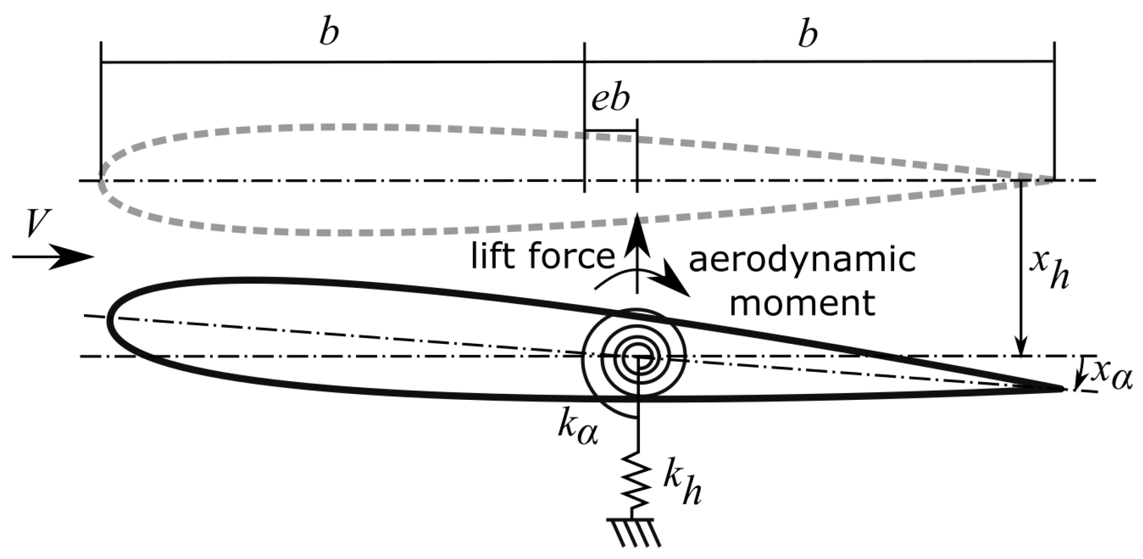
The 2-DOF typical section model constitutes a two-dimensional airfoil section with a plunge and pitch degrees of freedom, denoted with subscripts
h and
, in incompressible flow; see
Figure 1. The air loads are described by the lift force and the aerodynamic moment around the elastic axis, where the section model is elastically restrained with a vertical stiffness
and a torsional stiffness
. Therefore, the nonlinear aeroelastic eigenproblem for the typical section model results in
where the mass matrix includes the total mass
m, the first moment of mass
around the elastic axis and the moment of inertia
. The aerodynamic transfer function matrix
provides the negative lift force and the aerodynamic moment in the Laplace domain from the amplitudes of motion
,
. Based on Theodorsen’s aerodynamic airfoil theory [
19], commonly described in the aeroelastic literature [
22,
23], the unsteady aerodynamic forces are extended for growing and decaying oscillations by employing the generalized Theodorsen function
[
20]. Expressed in dimensional form with reference to the unit span of the section, the aerodynamic transfer function matrix is given by
which includes the dynamic pressure
and the area per unit span
. The reference length
L for the reduced frequencies is the half chord length
b. The elastic axis is positioned relative to the mid-point by the nondimensional parameter
e. The generalized Theodorsen function
is provided in Equation (
A5) in
Appendix B.
The aerodynamic transfer function matrix for the
p-
k method
is found by evaluation of Equation (
33) with
, neglecting the real part of the reduced complex-valued frequency
; see Equation (
4). For the
g method, in Equation (
5), the additionally required partial derivative
is obtained by applying the analytic property of
at
, relating
where
, given in Equation (
A1) in
Appendix A, requires the derivative of the generalized Theodorsen function derived in
Appendix B.
The employed parameter values for the section model are listed in
Table 1.
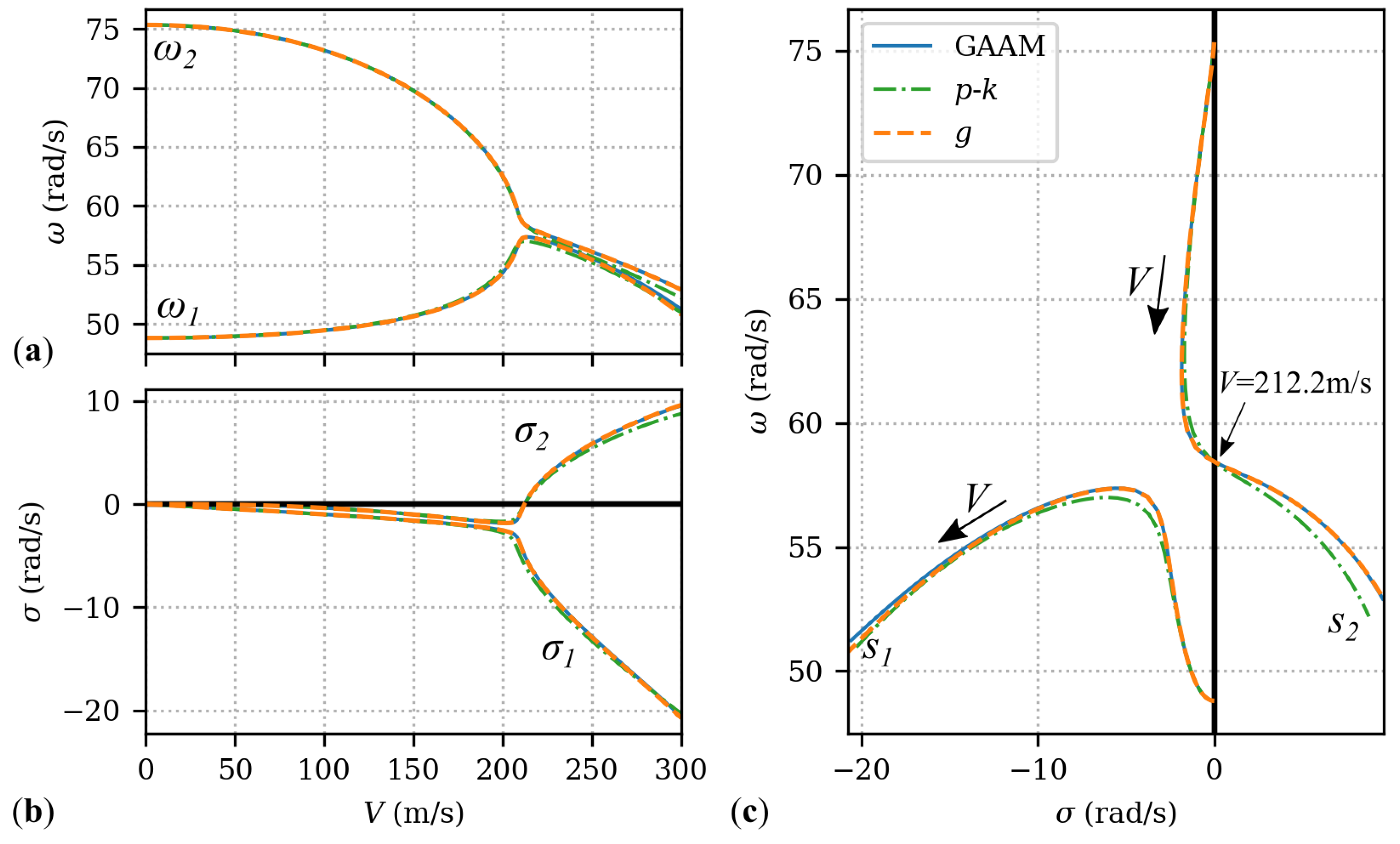
In
Figure 2, the eigenvalue solutions for the section model obtained by the
p-
k method, the
g method and GAAM are shown over a velocity sweep from 0 m/s to 300 m/s. Overall, the three methods yield similar results. From
Figure 2b,c, the flutter onset is found for the second eigenvalue
, where the real part
is zero at the freestream velocity
m/s. As expected, the flutter onset is identically identified by all three methods. However, for other velocities where
, the eigenvalue solutions exhibit slight variations. For the
p-
k method, the differences are more pronounced, while the
g method deviates little from GAAM. In fact, for high velocities where
sufficiently increases from zero, small deviations for the
g method are observed. These results confirm the main distinction between the aerodynamic damping approximations in which the real part of the Laplace variable is included to different degrees.
At each velocity, the derivatives of the eigenvalue solutions with respect to a design parameter are obtained by employing the direct method; see
Section 3.2. The design parameter for the verification of the derived equations is selected to be the half chord length
b. Hence, the quantities of interest are how the eigenvalues change with changing
b. Varying the half chord length implies a change in shape, requiring the partial derivative of the aerodynamic transfer function matrix
. Moreover, since the half chord length is the reference length, the additional terms regarding the partial derivative of the reduced frequency with respect to
L are included. Therefore, the design parameter
b is well suited to verify the derived eigenvalue derivatives. However, the structural derivatives with respect to
b are neglected in the following verification and the structural parameters are considered to be independent of
b.
In order to obtain the eigenvalue derivatives, GAAM requires the partial derivatives
and
, given by Equations (
A1) and (
A2) in
Appendix A. The partial derivative
, for the
p-
k and
g methods, is the derivative
, where the real part
is neglected. The
g method additionally requires the second-order partial derivatives
and
, as discussed in
Section 3.4. These are again obtained from the analytic property of
, resulting in
where the second-order partial derivatives of
are evaluated at
.
For the verification, the half chord length of the section model is changed by step sizes
ranging from 1 × 10
m to
m. Subsequently, for a given velocity, the eigenvalue solutions for each modified section model are obtained by solving the nonlinear eigenproblem.
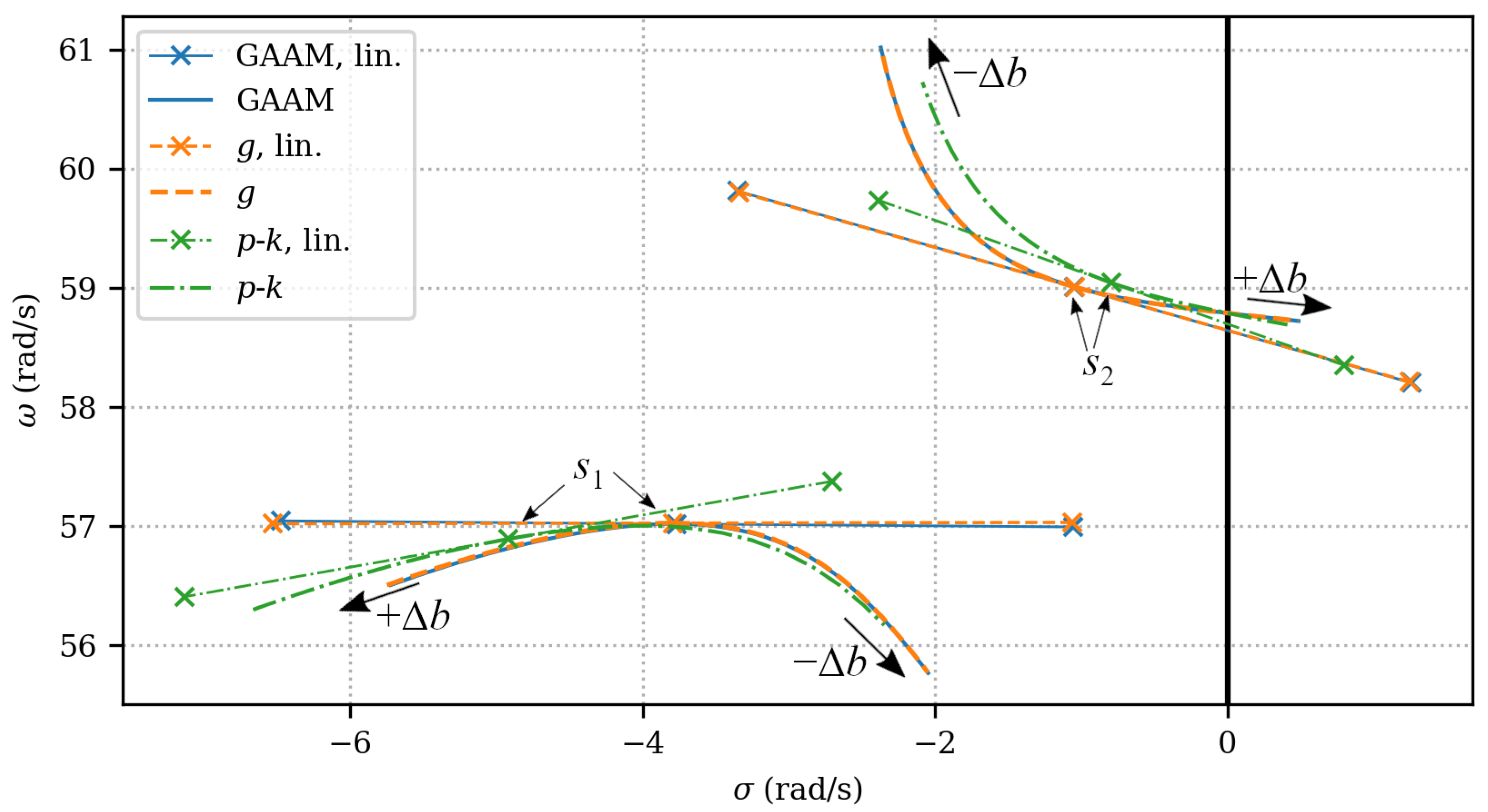
Figure 3 displays the change in the eigenvalues for changing half chord length by
at a freestream velocity
m/s. The velocity is close to the flutter onset and, thus, the eigenvalue
is close to the imaginary axis where
. To illustrate the results, at this velocity, the second eigenvalue would become less stable with increasing half chord length and eventually become unstable. Additionally, the predicted linear changes in the eigenvalues by the eigenvalue derivatives are shown as lines attached to the eigenvalues of the unchanged section model. The depicted lines display the scaled eigenvalue derivatives by multiplication with
. From visual judgement, the resulting tangent lines show very good agreement with the slopes of the nonlinear curves at the solution of the unchanged model. In addition to the visual comparison, the numerical values of the obtained eigenvalue derivatives are given in
Table 2.
By comparing the result between the
p-
k method,
g method and GAAM in
Figure 3, the difference in the eigenvalue solution for the unchanged section model is noted, as is also shown in
Figure 2. This difference is more pronounced at
with greater distance from the imaginary axis. Hence, the nonlinearly changing eigenvalues exhibit differences, which are the greatest for the
p-
k method, since the unchanged eigenvalue solution already shows the greatest offset. The
g method shows very little difference to GAAM for the nonlinearly and linearly obtained second eigenvalues
. For the first eigenvalue, a small offset in the unchanged eigenvalue is observed, with little differences in the nonlinearly obtained eigenvalues for greater values of
. Although the unchanged eigenvalues for the
g method and GAAM are very close, a small but visible difference in the visualized eigenvalue derivatives at the first eigenvalue is observed, as reported in
Table 2, reflecting the difference in the underlying aerodynamic damping approximation. This is one of the main results of the current work, pointing out the effect of the aerodynamic damping approximation on the aeroelastic eigensensitivities, even though the predicted eigensolution to the flutter equation is very similar.
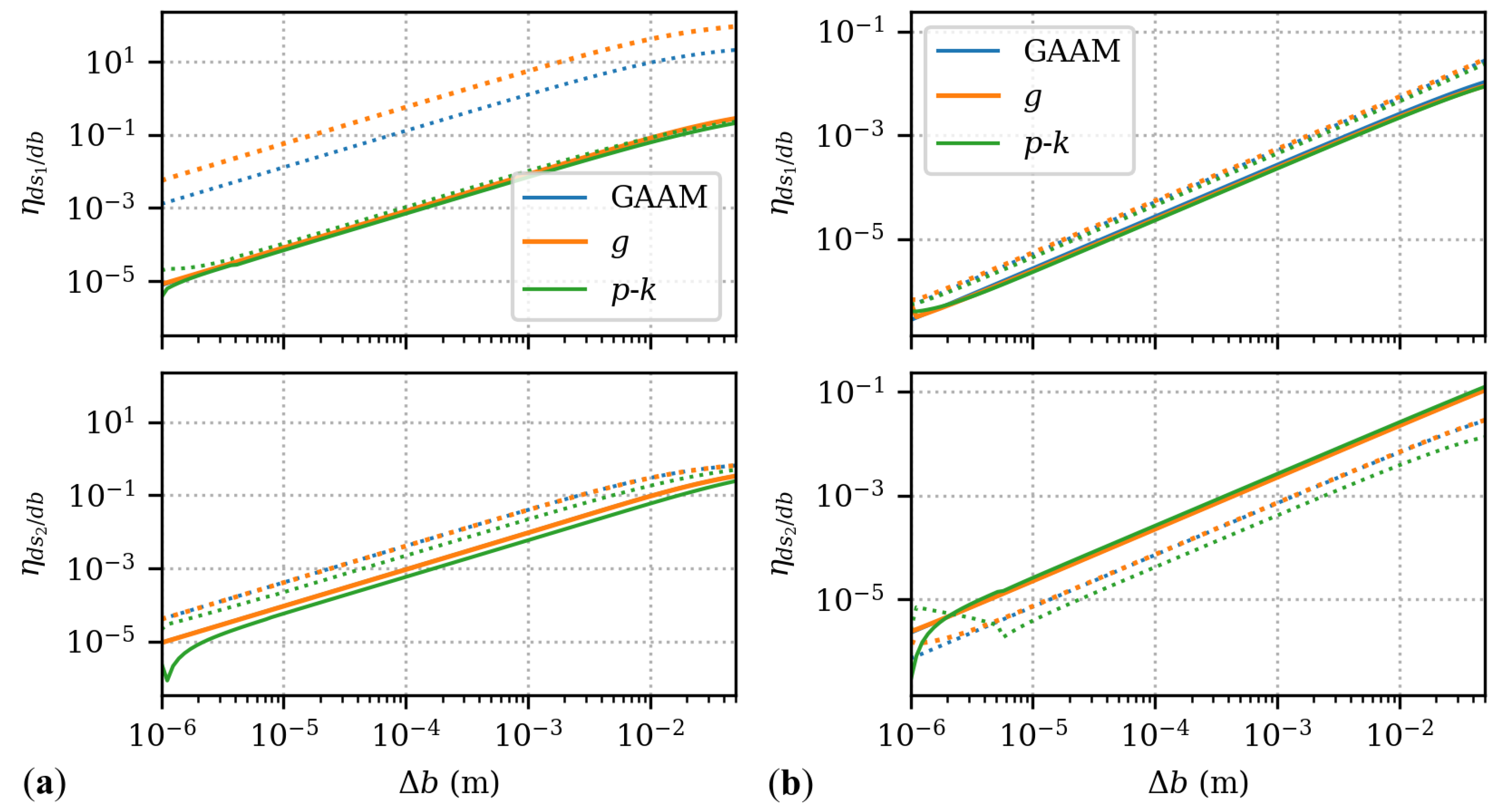
Finally, the derived analytical eigenvalue derivatives are verified by the analysis of the relative error to forward finite difference approximations. Considering the eigenvalues as a function of
renders the finite difference approximations using nonlinearly obtained eigenvalues evaluated at
. Subsequently, the relative error is given by
where the latter equality results from Taylor’s theorem, leading to a first-order approximation error if the evaluated derivatives are the analytical derivatives. Consequently, the relative error converges linearly with decreasing
for the analytical derivatives.
Figure 4 displays the relative errors of Equation (
34) for the eigenvalue derivatives at two freestream velocities
m/s and
m/s. For the three investigated aerodynamic damping approximations, the relative errors separated in real and imaginary parts exhibit an exponential decline for the decreasing step size
. Examining the slopes shows a first-order reduction in the relative error, which is in line with the stated condition for analytical derivatives in Equation (
34). For very small step sizes
, the relative error deviates from the first-order reduction because of the increasing numerical error in the finite difference approximations due to numerical cancellation. From these results, it is concluded that the obtained eigenvalue derivatives are in agreement with the finite difference approximations, verifying the derived equations for the eigenvalue sensitivities.
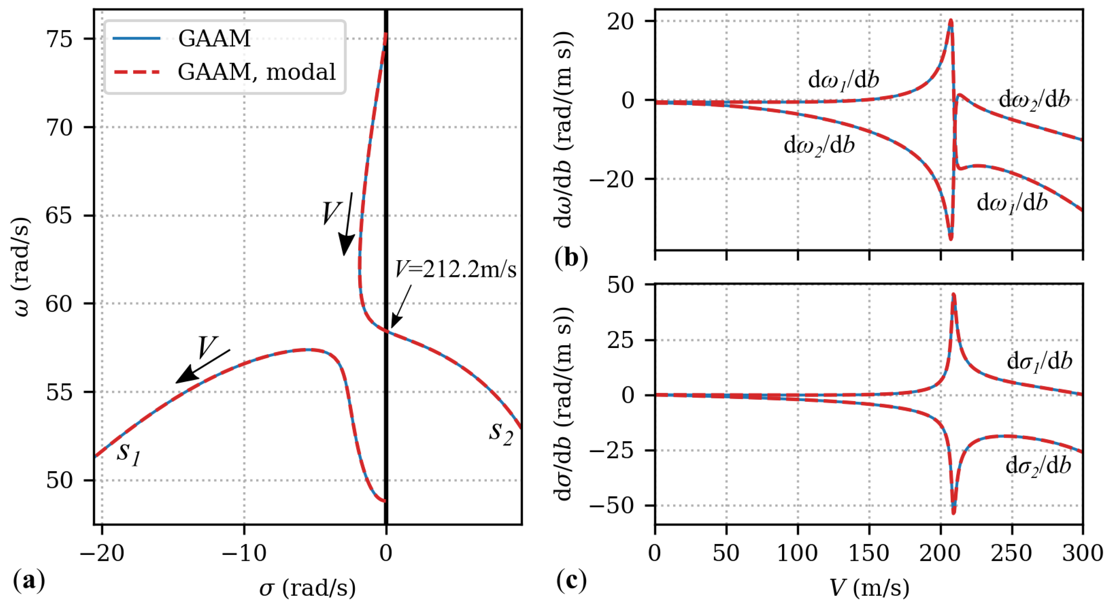
To this end, it remains to verify the eigenvalue sensitivities employing modal coordinates. For this, it is sufficient to compare the eigenvalue derivatives obtained in modal coordinates without modal truncation to the verified solutions obtained in physical coordinates.
Figure 5 shows this comparison for the design parameter
b employing GAAM. In
Figure 5a, the eigenvalue solutions are displayed for a velocity sweep from 0 m/s to 300 m/s.
Figure 5b,c show the real and imaginary parts of the eigenvalue derivatives at each velocity. The eigenvalue derivatives are obtained by the direct method in physical coordinates—see Equation (
14)—and in modal coordinates—see Equation (
15). No differences are observed in
Figure 5, verifying the equality of the solutions of the direct method in physical and modal coordinates without modal truncation.
4.2. Aeroelastic Sensitivities of the AGARD 445.6 Wing
In this section, the derived aeroelastic sensitivities are applied to the AGARD 445.6 weakened wing model for varying wing sweep. The AGARD 445.6 weakened wing model is a widely known aeroelastic test case [
24,
25]. It is a swept wing clamped at the wing root with a quarter chord sweep of
, a root chord length of
m, a span of 0.762 m and a taper ratio of 0.66. The model comprises a finite element model (FEM) with 200 shell elements and a doublet lattice model (DLM) with 200 boxes, which both are obtained from [
26] for a Mach number of 0.9 and air density
= 0.31 kg/m
3.
The commercial solver MSC Nastran [
7] is employed in order to extract the mass matrix
and stiffness matrix
as well as the modal matrix
by performing a linear modal analysis. In this model, the first four structural mode shapes are considered, which are the first wing bending and first wing torsion, followed by the second wing bending and second wing torsion. The structural eigenfrequencies are listed in
Table 3 together with the parameter values. Furthermore, the aerodynamic transfer function matrices
employing DLM are extracted from MSC Nastran, sampled at 17 reduced frequencies
ranging from 0.001 to 5, clustered densely in the region up to 1. An interpolation method based on piecewise cubic functions provides the evaluation of
at additional frequencies, which are required in obtaining the eigenvalue solutions. Moreover, the interpolation method enables the efficient evaluation of the derivatives of
with respect to
, which are, therefore, continuous up to the second order. The aerodynamic transfer function matrices include the spline matrix, which is required for mapping the structural displacement onto the aerodynamic grid as well as the aerodynamic forces onto the structural grid using infinite plate spline interpolation [
27]. Taken together, the extracted matrices allow us to solve the nonlinear aeroelastic eigenproblem in modal coordinates; cf. Equation (
2).
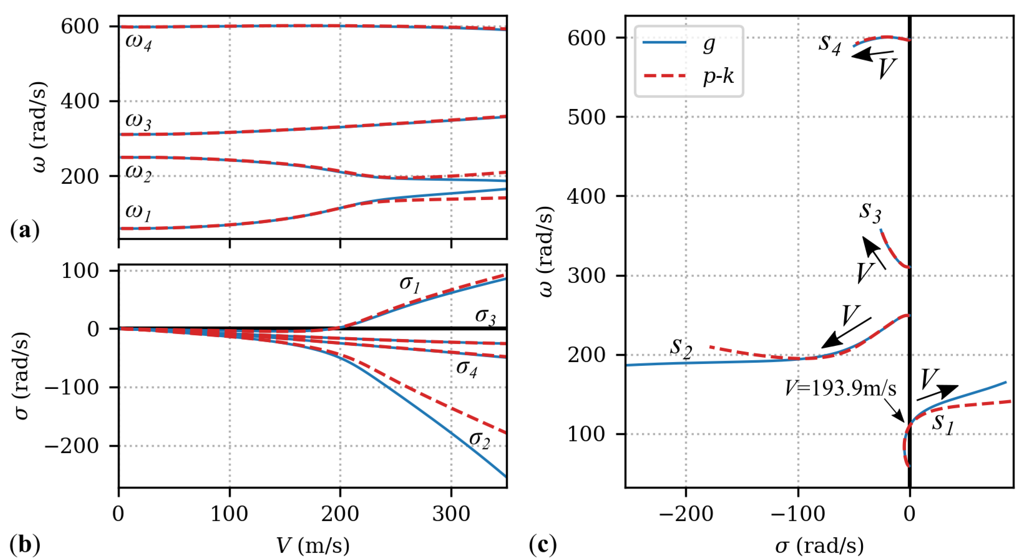
In
Figure 6, the eigenvalue solutions for the AGARD 445.6 weakened model obtained by the
p-
k method and the
g method are shown over a velocity sweep from 0 m/s to 350 m/s. The flutter onset is found by both methods for the first eigenvalue
at the freestream velocity
m/s, as shown in
Figure 6b,c. For smaller freestream velocities, the
p-
k method and the
g method yield very similar solutions. The solutions start to differ for higher freestream velocities, where the real part of the eigenvalues
increases. This is most pronounced for the first and second eigenvalues,
and
, which exhibit the most damping and, thus, significant deviations between both methods are observed for freestream velocities greater than the flutter onset velocity.
The sweep angle of the AGARD 445.6 weakened model is varied by applying a shear transformation for a step size
without affecting the other parameters, such as root chord length, span and taper ratio. The sweep angle is changed for step sizes ranging from 4.67 × 10
to
. For each step size, MSC Nastran is employed for acquiring
,
,
and
, as described previously. Subsequently, the nonlinear aeroelastic eigenproblem is solved for each sweep angle in order to obtain the nonlinearly changing eigenvalues for varying sweep. Furthermore, the extracted mass matrix
and stiffness matrix
are used for forward finite difference approximations of the model sensitivities
and
. From these sensitivities, the sensitivity of the modal matrix
is obtained following
Section 3.5. Additionally, the sensitivity of the aerodynamic transfer function matrix
is determined by forward finite difference approximations for each sampled frequency. With these defined model sensitivities, the eigenvalue sensitivities are solved by employing the direct method for separated real and imaginary parts, as stated in Equation (
22) in model coordinates. Hence, the linear system of equations includes the additional terms regarding the derivative of the modal matrix; see Equation (
11).
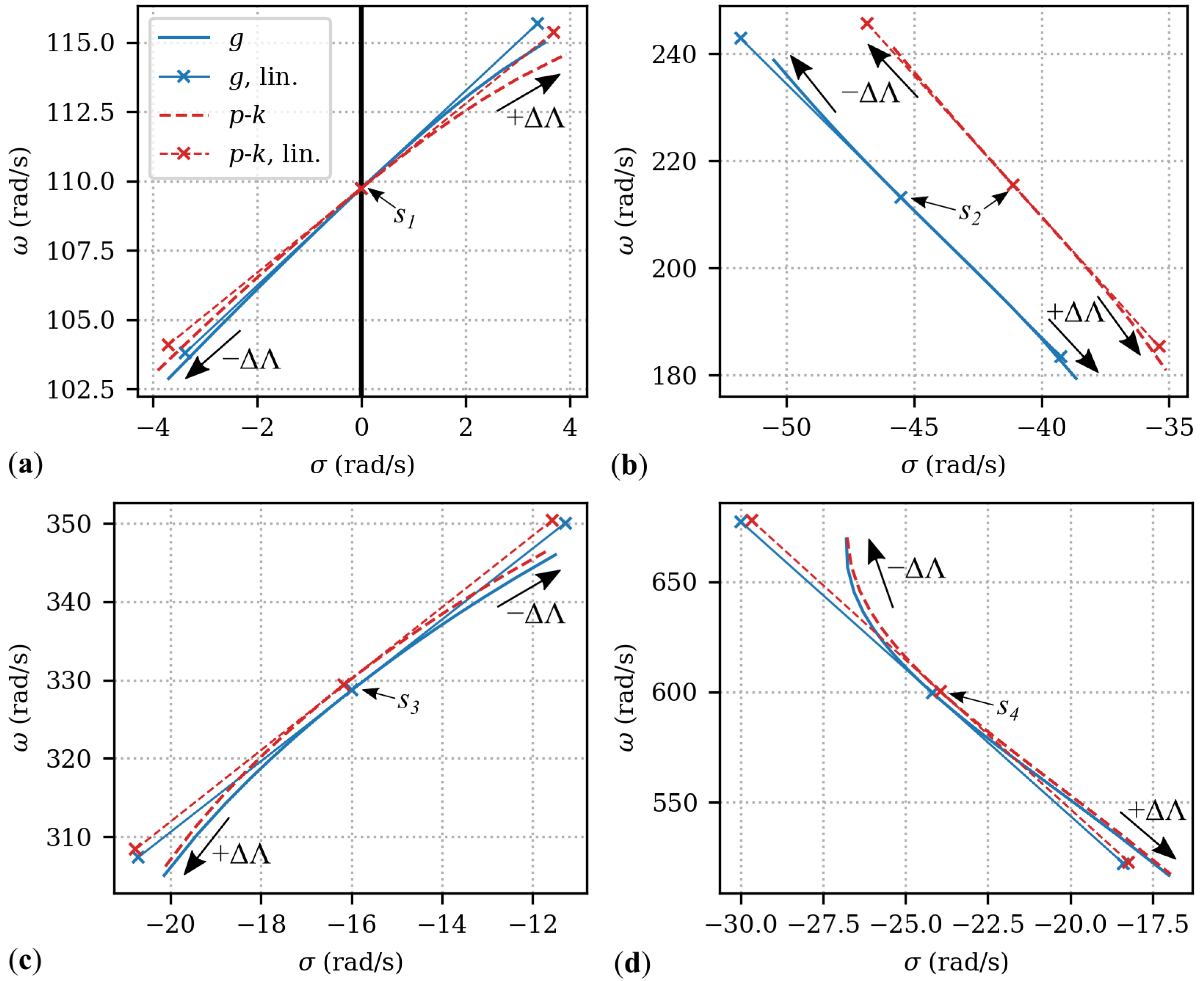
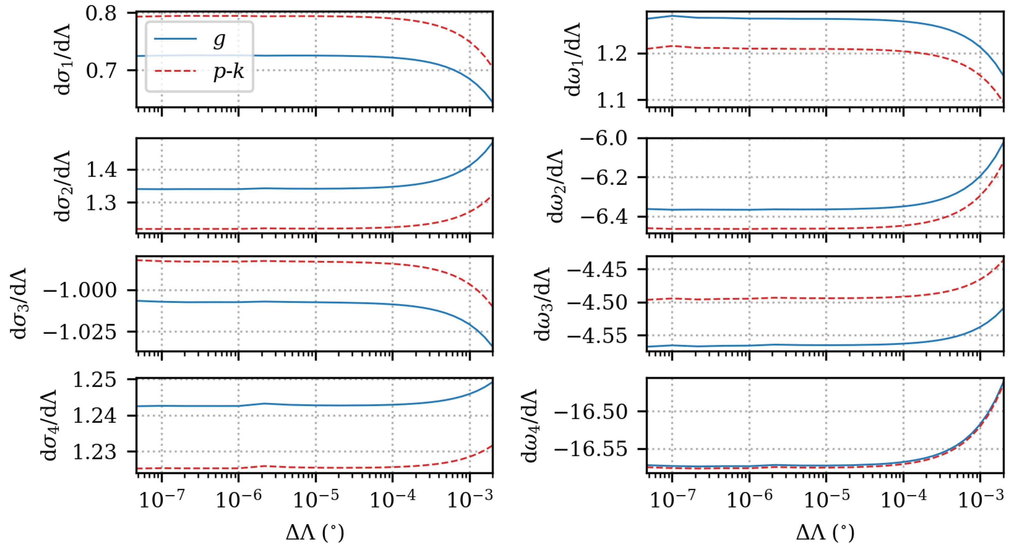
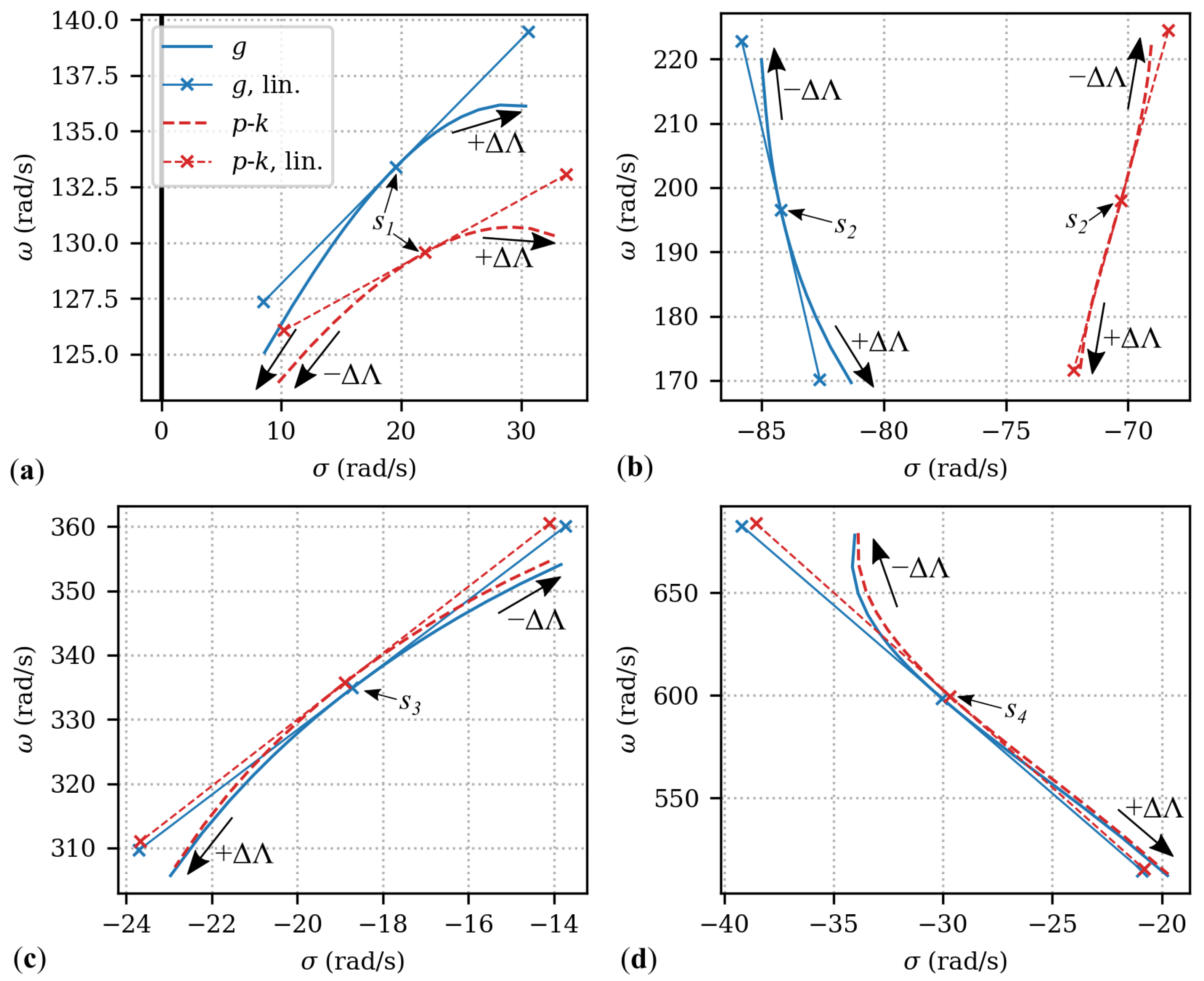
Figure 7 shows the nonlinearly changing eigenvalues as well as the predicted linear change from the eigenvalue sensitivities for varying sweep at the flutter onset velocity. Similar to
Section 4.1, the lines representing the eigenvalue sensitivities are defined by the multiplication of the eigenvalue sensitivities with
. The eigenvalue sensitivities are shown for the model sensitivities obtained for the step size
= 5.9 × 10
, resulting from a convergence study, shown in
Figure 8. For the flutter onset velocity, the
p-
k and
g methods yield the same eigenvalue
for the unchanged model, as is confirmed in
Figure 7a. However, the nonlinearly obtained eigenvalues for changing sweep differ for both methods, which is correctly reflected by the observed difference in the linearly predicted eigenvalues. Hence, the eigenvalue sensitivities are different for the
p-
k method and the
g method, although the eigenvalue solutions are the same and, moreover, have a real part of zero.
For the second eigenvalue
—see
Figure 7b—the difference between both methods results primarily from the offset between the eigenvalue solutions for the unchanged model. As a result, different eigenvalue sensitivities are obtained—see also
Figure 8, where numerical values are compared. The difference in the eigenvalue solutions of the third and fourth eigenvalue shown in
Figure 7c,d is less pronounced. This is in line with the previous observation that the first and second eigenvalues are more affected by the investigated aerodynamic damping approximations.
In
Figure 9, the eigenvalue solutions for changing sweep are shown for the freestream velocity
m/s, above the flutter onset. In this case, the difference between both methods results from the offset for the first and second eigenvalue,
and
, of the unchanged model. Moreover, the eigenvalue sensitivities as well as the nonlinearly obtained eigenvalues reveal the difference in the change in the aeroelastic stability resulting from the different aerodynamic damping approximations.


