Low Speed Aerodynamic Analysis of the N2A Hybrid Wing–Body

Abstract

Reduction of atmospheric emissions is currently a mandatory requirement for aircraft manufacturers. Several studies performed on Blended Wing–Body configurations showed a promising capability of reducing fuel consumption by increasing, at the same time, passengers’ transport capabilities. Although several aerodynamic studies are available at transonic speeds, low-speed evaluations of aerodynamic performances of Blended Wing Body aircrafts are less investigated. In this framework, the present paper deals with the aerodynamic performance of the N2A aircraft prototype at low-Mach number conditions. Aircraft longitudinal aerodynamics is addressed at $M_{\infty }=0.2$ with steady state three-dimensional RANS simulations carried out at two Reynolds numbers equal to $6.60\times {10}^6$ and $1.27\times {10}^8$, respectively. The former refers to an experimental test campaign performed at NASA Langley 14-by-22 foot subsonic tunnel, while the latter is related to free-flight conditions close to an approach and landing phase. Flowfield simulations are performed using the Computational Fluid Dynamic code FLUENT and the SU2 open-source code, currently adopted for research applications. Numerical solutions are validated by using available experimental data with reference to lift, drag, pitching moment and drag polar estimations. Pre-stall and post-stall aerodynamic behaviour through mean flow-field visualization along with the comparison of pressure distributions at several AoAs is addressed. Furthermore, the effect of convective discretization on a numerical solution for SU2 is discussed. Results indicate a good agreement with available experimental predictions. The present study aims to bridge existing computations at a Eulerian low-Mach number, with RANS computations and constitutes a further test-case for SU2 code with respect to a full aircraft configuration.

1. Introduction

The mandatory urge to reduce atmospheric emissions caused by the recent climate changes has also been reflecting on the design of commercial aviation aircrafts. It was estimated in the past that emissions from commercial aviation have been quantified to be two or three percent of the total emissions [1]. However, as this percentage is expected to rapidly increase in the upcoming future, the design of fuel saving configurations is currently being considered.

Several conceptual studies performed by McDonnell Douglas, and the joint collaboration of NASA and Boeing, demonstrated that Blended Wing–Body (BWB) aircraft represent promising configurations to improve aerodynamic efficiency and to reduce fuel consumption compared to the conventional Tube and Wing (TAW) configurations [2,3]. BWB is a hybrid aeroshape which integrates the concept of a uniform lifting body seamlessly compenetrated with an airfoil-shaped fuselage. The aerodynamic advantage of the BWB design relies on its lower wetted area to volume ratio and its Sears–Haack like body cross sections [4]. The BWB design provides a lower skin friction drag and a lower interference drag, driving to an increase of aircraft aerodynamic efficiency [5]. Additionally, because of the smoother wing-fuselage integration, it allows for increasing the passenger transport capabilities. Furthermore, the integration of the engine in the rear part of the lifting body improves the noise shielding.

Although BWB configuration has several advantages, such design is affected by a reduced longitudinal control authority due to the absence of the horizontal stabiliser. More precisely, BWB has no separate horizontal and vertical stabilizer. The longitudinal stability is ensured by reducing the aerodynamic load on the center body [3]. Additionally, directional stability is obtained with winglets and/or vertical tails, but inevitably the control authority is relaxed [1].

Finally, non circular cross-sections can be subjected to structural problems related to cabin pressurization. Because BWB is optimally designed for transonic cruise speed ($M_{\infty }=0.8$), the reduced control authority can compromise landing or take-off phases in the presence of external aerodynamic disturbances [1]. Therefore, earlier BWB concepts by Northrop in 1930s to the mid 1950s were abandoned.

In the recent years, BWB design is reconsidered because of the strict mandatory reduction of NO_x and CO₂ emissions required for aircraft industries. In this framework, it is worth emphasizing the activities of the German Cluster for Sustainable and Efficient Energy Aviation [5]. The program is actually aimed at finding mutual influence between brand new aircraft configurations and the development of new technologies over atmospheric emissions.

Current research activities on BWB demonstrate that the coupling of high fidelity aerodynamics (Eulerian- or RANS-based) with optimization procedures can improve BWB aircraft (drag) performances [4,6,7]. Specifically, trade-offs between aerodynamics, stability and structural constraints enable new design solutions, eventually driving to drag reduction [4]. Because computing facilities made it possible to perform Euler or RANS-based simulations inside optimization loops, several toolkits specifically developed for aerodynamic simulations become effective for BWB design [8].

In this scenario, affordable and less time-consuming numerical codes with robust numerical schemes and accurate domain discretizations are of fundamental importance to have a reliable design tool to feed Multidisciplinary Design Optimization (MDO) procedures [6,9,10]. With this in mind, the present study focuses on the aerodynamic analysis of a BWB prototype, namely N2A, at low-Mach number conditions with the aim to explore and assess the accuracy of flowfield simulations carried out with grids built with about 15 M cells (half body), suitable for MDO procedures. Although several previous CFD studies on BWB are available at cruise speed conditions [2,3,11,12,13], research literature shows that subsonic aerodynamics need to be further investigated, especially at approach and landing speeds. Two CFD tools, namely ANSYS-FLUENT and SU2 (v7.2.0 Blackbird), are adopted and compared with both experimental wind tunnel (WT) data and with other CFD simulations available in literature [6,14]. SU2 code is gaining a growing attention from the research community focused on aerodynamic design. SU2 is released under an open-source licence, and it is constituted by several pre-compiled CFD solvers and PDE-constrained optimization algorithms [8].

In the present framework, first the consolidated solver FLUENT is adopted and compared with experimental WT data to address convergence properties of numerical solutions with respect to the grid resolution and numerical discretisation adopted. The lift and drag coefficients, drag polar and pitching moment coefficients are computed at several angle of attacks (AoAs) with steady state RANS simulations. The same computations are then performed with the SU2 toolkit.

The data gathered make an interesting validation case due to the unconventional aeroshape and allows for bridging the existing CFD results, available in literature for transonic Mach numbers, with the low-subsonic ones. Additionally, it will shed light on the potential capability of SU2 work to be employed to build several computations for a complete aircraft configuration.

2. Related Work

Performances of BWB aircrafts are investigated in literature with massive use of CFD simulations. It is worth noting that optimal aerodynamic performances of BWB are obtained at transonic speed. Therefore, the majority of CFD studies available in literature refer to this flight condition.

Early numerical assessments of BWB compared to experimental data were carried out using a NASA transonic wind tunnel by Liebeck [11,12]. Good fit with experimental data were found for all aerodynamic coefficients. Aerodynamic performance of BWB at $M_{\infty }=0.85$ were analysed in Qin et al. [3]. Panel method and RANS simulation were jointly used in an inverse twist design method to reduce drag coefficient. A lift coefficient for untwisted wing planform was evaluated with panel methods. Then, local wing sections were twisted to match potential field computations deriving a correction factor for spanwise lift distribution. RANS simulation was then used to evaluate viscous contribution. Optimization runs for a minimum drag objective showed the major impact over the design of pressure drag. Deere et al. [13] focused on the aerodynamic predictions of a Hybrid Wing–Body (HWB) to simulate transonic cruise condition. Three different configurations of the same BWB were considered in order to evaluate the influence of engines over global aerodynamic prediction: (i) complete aircraft configuration; (ii) the wing–body tail configuration; (iii) and the isolated nacelle configuration. Aerodynamic performance was found to be sensitive to the spanwise loading distribution resulting from the coupled effect of engine interference. Comparisons performed between RANS codes adopted by NASA and Boeing showed only minor differences ascribed to different turbulence models.

Currently, research on BWB integrates high fidelity CFD data into optimization procedures because of the increased computational power, which allows both Euler and RANS-based computation.

Almosnino [6] performed a first evaluation of low-subsonic performance of NASA’s N2A wing–body configuration. Specifically, inviscid computations performed with an adjoint solver were performed and compared to experimental data. Results showed good agreement for the lift coefficient, while the drag coefficient was underestimated, of course. It was concluded that, due to a stiffness problem associated with the low-Mach condition, the grid resolution was not sufficiently refined to accurately predict drag.

Martins at al. [4] exploited RANS-data driven optimizations to trade-off aerodynamic and stability characteristics of a BWB configuration. Geometric design variables, like planform area and airfoil shape, were considered as constraints. The adoption of CFD data in an optimization loop demonstrates a reduction of the drag coefficient both in single- and multi-point optimization, thus also suggesting a lower planform area.

Karpuk et al. [5] developed a design approach with a different fidelity level for a fuel-efficient BWB aircraft. The multi-fidelity aerodynamic was based on an AVL tool for low-fidelity levels while SU2 coupled to the FFD approach to change geometry was adopted for high fidelity computations. These tools were integrated in a common framework to improve aerodynamic efficiency. Although lift was fairly predicted by the two approaches, underestimation of transonic drag coefficients with AVL were instead detected by SU2.

Additionally, WT experimental test campaigns are also available for the N2A aeroshape. They have provided a comprehensive dataset of the low speed aerodynamic performance of this aircraft [14,15,16].

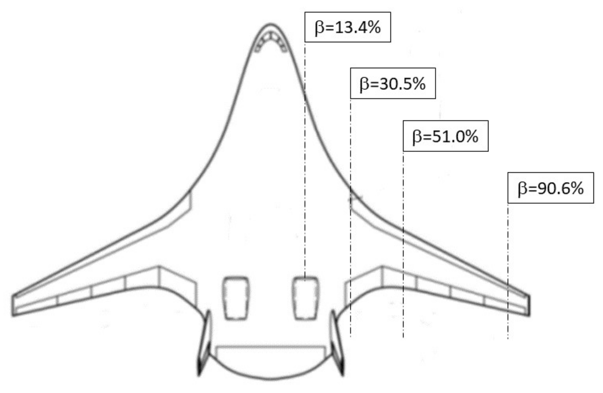
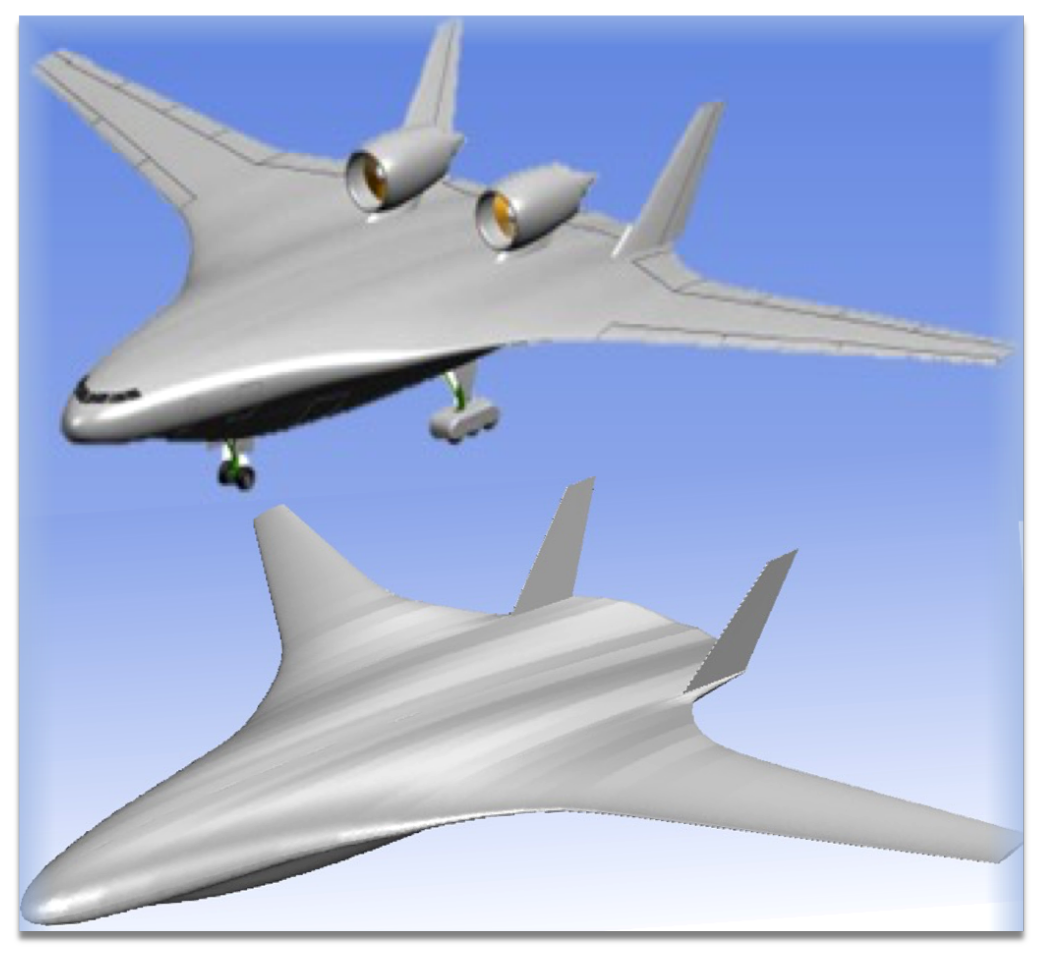
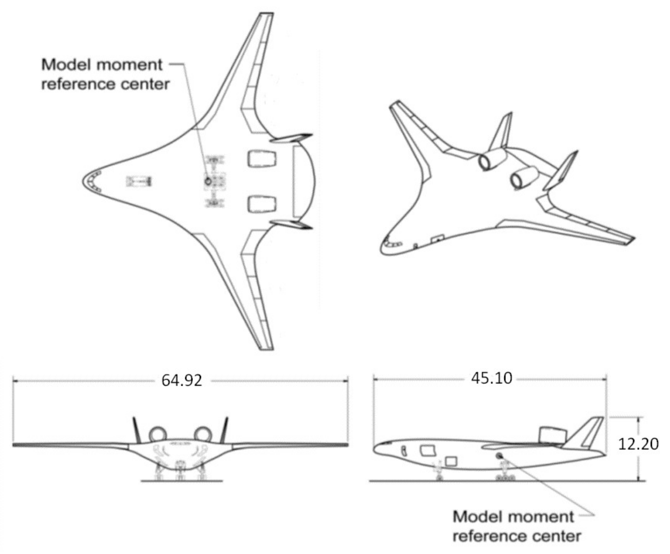
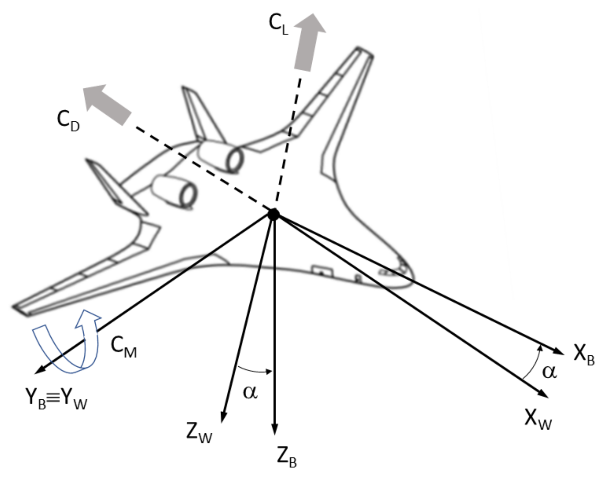
3. Aircraft Aeroshape and Aerodynamics

The aircraft aeroshape under investigation is shown in Figure 1. Specifically, in the upper detail of the figure, the realistic aircraft configuration is provided, while, in the lower part of Figure 1, the studied configuration is shown. Neither nacelles nor landing gears are considered for the sake of simplicity. This water-tight aeroshape is provided by the NASA code OpenVSP [17].

The N2A aircraft features a HWB configuration incorporating twin, podded nacelles mounted on the aircraft leeside, close to two low Aspect Ratio (AR) vertical tails. This aeroshape was derived by a NASA Research Announcement (NRA) aimed at developing an efficient low-noise HWB subsonic transport aircraft [18]. NRA was also aimed to meet the goals of both fuel and noise reductions, and additionally to study the subsonic aerodynamics performance of the HBW configuration [14,15,16].

With this in mind, several WT tests were carried out in the NASA Langley 14-by-22 foot subsonic tunnel on the 5.8% scale model of N2A aircraft. Two sets of WT data are available for comparison, namely the cruise configuration and the baseline configuration. The former is the N2A wing–body configuration, without fins and nacelles, and with no dropped leading edge. The latter (i.e., baseline configuration) is the full N2A configuration. Therefore, present CFD results will be compared with literature data available for the cruise configuration.

Longitudinal aerodynamic coefficients of the aircraft as well as pressure distribution along with selected spanwise locations are evaluated and compared.

A three views drawing of the aircraft configuration is provided in Figure 2. As shown, the N2A configuration under investigation refers to clean configuration (i.e., all elevons and rudder undeflected); landing gear off; nacelles at the mid location; and the vertical tails mounted with a ${10}^{\circ }$ cant angle at the aft location [14]. The wing span is 64.92 m, while the body length is 45.10 m long. Furthermore, the sweep angle at the quarter-chord of the constant sweep, the outboard portion of the wing, is $24.2^{\circ }$. Then, a negative wing twist of $-8.{87}^{\circ }$ is provided at the wing tip through a linear variation. The wing thickness taper (i.e., $t/c$) is ∼$8\%$.

Aircraft aerodynamics rely on the ISO 1151 standard. Therefore, force and moment coefficients are provided according to Figure 3, where both body and wind reference frames are provided together with sign definitions for lift, drag and pitching moment coefficients.

Aeroshape reference area reads $S_{ref}=925.2{\mathrm{m}}^2$, while the reference length is $L_{ref}=26.52\mathrm{m}$.

Finally, the moment reference centre is located at 24.33 m aft of the aircraft nose (i.e., $53.94\%$ of the fuselage length).

4. CFD Simulation of the N2A Configuration

In order to address the aerodynamic performance of the N2A configuration, both the ANSYS-FLUENT and open-source code SU2 were adopted and compared.

Both experimental results and previous CFD studies performed with the CART3D solver are also available [6]. Air is modelled as perfect gas, with viscosity given by Sutherland law and specific heat at constant pressure equal to Cp = 1006 J/kgK. Air thermal conductivity is assumed constant, k = 0.0242 W/mK. The adiabatic wall boundary condition is applied on the vehicle aeroshape, while the pressure farfield and the pressure outlet boundary conditions are used at the domain inlet and outlet, respectively. RANS closure is performed by using the Shear Stress Transport (SST) $k-\omega$ model.

4.1. CFD Test Matrix

Aircraft aerodynamics have been addressed according to the test matrix summarized in

Table 1. CFD Test matrix for free-flight ($R{e}_{L_{ref}}$ = 1.27 $\times {10}^8$) and WT test ($R{e}_{L_{ref}}$ = 6.60 ×${10}^6$) conditions.

AoA (deg)	${\mathit{M}}_{\mathit{\infty }}$ (-)	${\mathit{Re}}_{{\mathit{L}}_{\mathit{ref}}}$$\times {10}^8$ (-)	SU2	FLUENT	${\mathit{Re}}_{{\mathit{L}}_{\mathit{ref}}}$$\times {10}^6$ (-)	SU2	FLUENT
−5.00	0.20	1.27	x	x	6.60	x	x
−2.50	0.20	1.27			6.60		x
0.00	0.20	1.27	x	x	6.60	x	x
2.50	0.20	1.27			6.60		x
5.00	0.20	1.27		x	6.60	x	x
8.36	0.20	1.27	x		6.60	x	x
10.00	0.20	1.27	x	x	6.60		x
13.00	0.20	1.27		x	6.60		x
15.00	0.20	1.27	x	x	6.60		x
20.00	0.20	1.27		x	6.60		x

, where “x” denotes whether simulation has been performed at selected AoA.

As shown, two flight conditions have been considered in addressing aircraft aerodynamics, namely WT test (i.e., $R{e}_{L_{ref}}=6.60\times {10}^6$) and free-flight (FF) (i.e., $R{e}_{L_{ref}}=1.27\times {10}^8$) conditions. Moreover, according to Ref. [16], there are two WT tests, namely T597 conducted with a closed test section and T612, which refers to measurements conducted with an open test section. Some data of both these tests are considered hereinafter for the assessment of the reliability of the present numerical research effort.

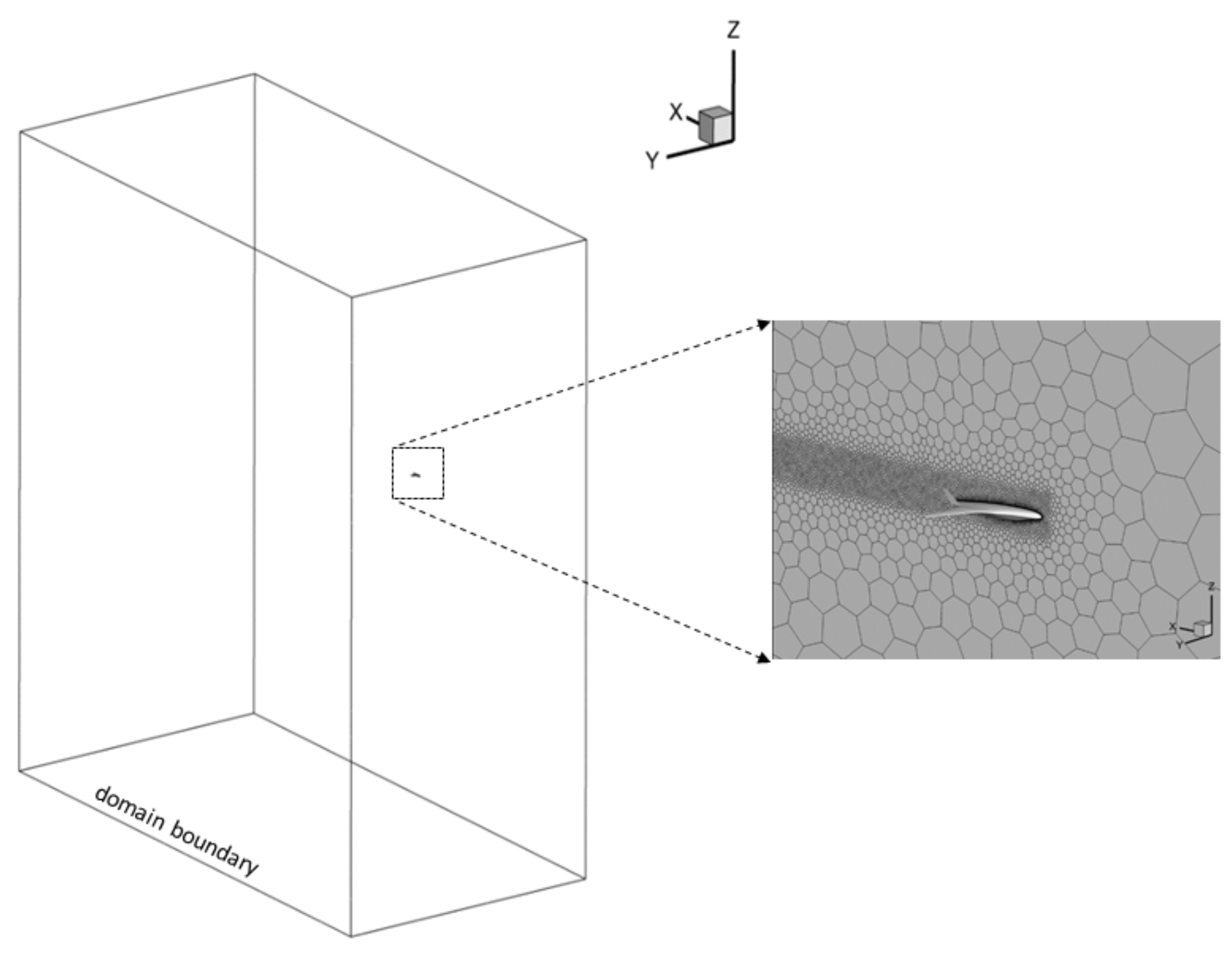
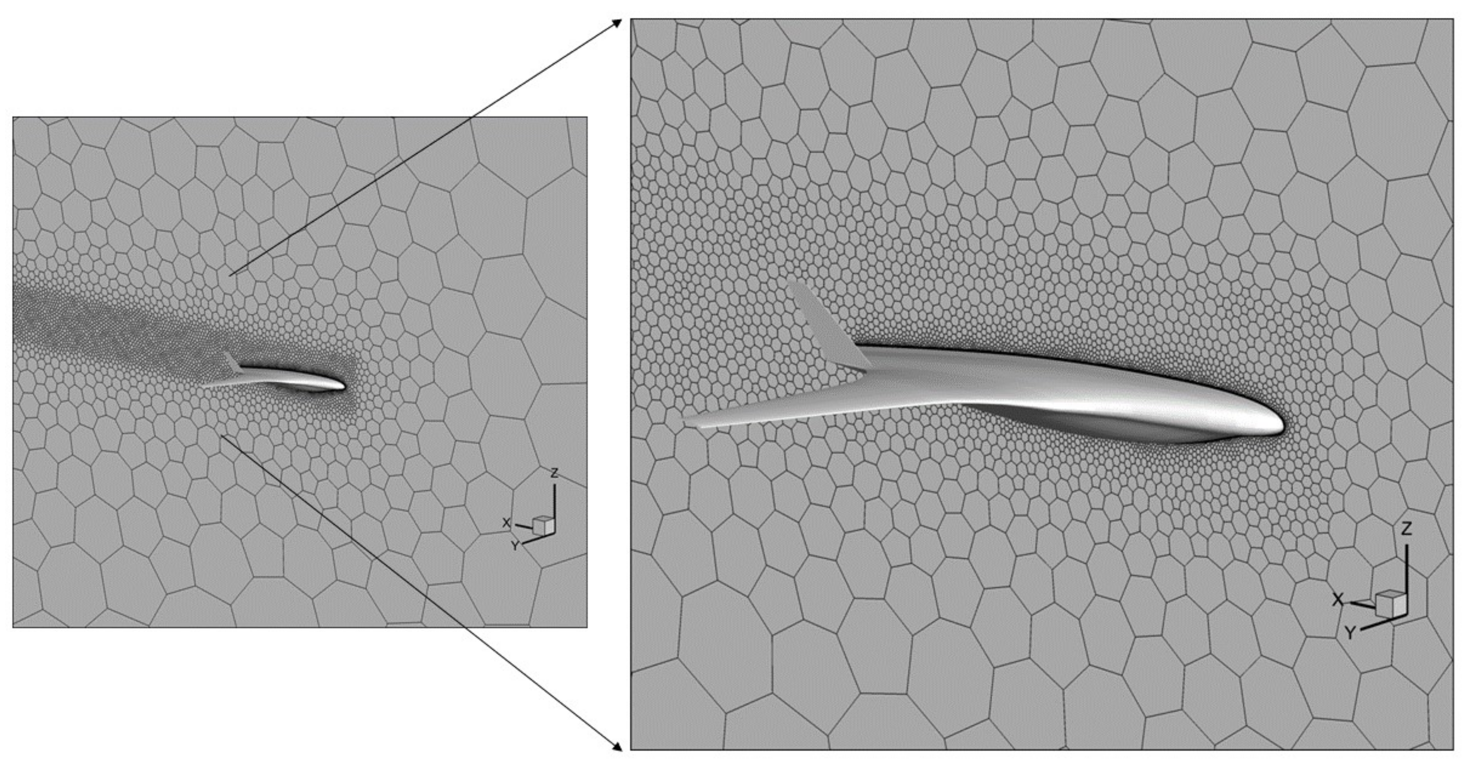
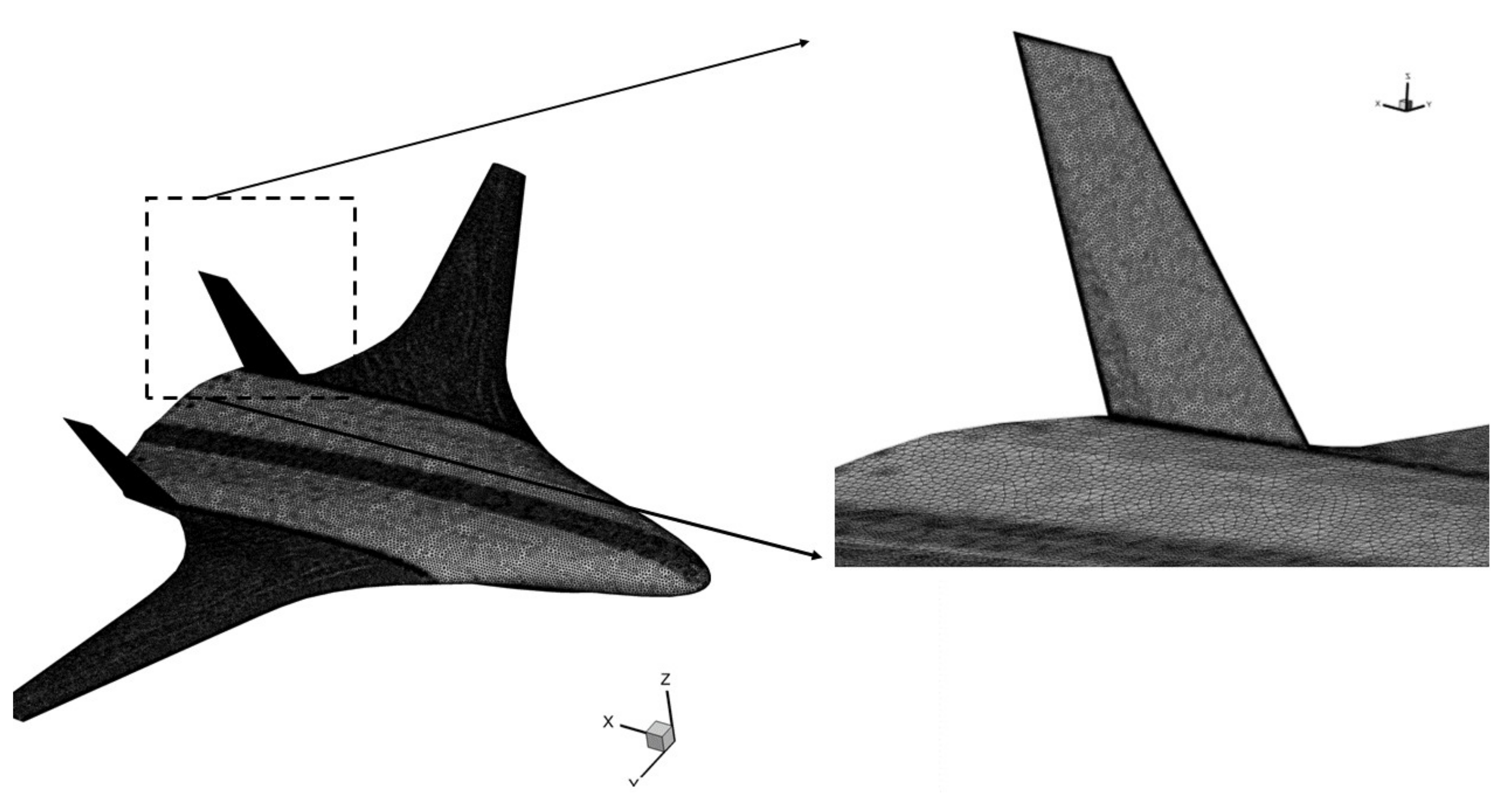
4.2. CFD Mesh Domain

Flowfield investigations have been carried out on hybrid grids, close to those shown in Figure 4, Figure 5 and Figure 6. The computational domain is provided in Figure 4.

As shown, the rather low free-stream Mach number demands a wide domain in order to avoid reflections of spurious numerical modes arising from the interference of the aircraft body with the domain boundaries. Specifically, the farfield boundary condition has been set at about fifty body lengths both upstream and downstream the aircraft (see Figure 4). Figure 5 shows the unstructured grid on the airplane symmetry plane. Clearly visible is the body of influence surrounding the aeroshape that has been used to allow refinements, thus improving the mesh close to the body.

The developed grids feature polyhedral cells in the field and prism inflation layers in the boundary layer, with enough points to describe the viscous sublayer and allow $Y^{+}=O\left(1\right)$ at the body surface to accurately predict velocity and temperature gradients normal to wall. Mesh domains with tetrahedral and prism cells have been previously built using the commercial tool ICEM-CFD, while conversion to polyhedral cells has been obtained using Fluent and preserving the prisms in the boundary layer.

An overview of the unstructured triangular mesh on the airplane surface is provided in Figure 6, where a detail of the mesh on the portside of the left vertical tail is also included.

The adopted grid resolution has been determined performing a grid convergence study, summarized in

Table 2. Grid convergence study at $\alpha$ = 0 deg and AoA = 0 deg.

Mesh	Cells, Half Body	${\mathit{C}}_{\mathit{L}}$	${\mathit{C}}_{\mathit{D}}$	$\mathit{ϵ}\left({\mathit{C}}_{\mathit{L}}\right)\%$	$\mathit{ϵ}\left({\mathit{C}}_{\mathit{D}}\right)\%$
Coarse	6610108	−0.0188	0.00654	9.30	5.31
Medium	14408538	−0.0175	0.00639	1.74	2.90
Fine	16544006	−0.0172	0.00621	-	-

, considering three different hybrid grids (half body), namely Coarse, Medium and Fine mesh. As shown, the number of cells of the medium grid is double the one adopted for the coarse mesh, as usual. However, the fine grid features only about 2.5 M more cells than the medium mesh. Note that the maximum number of about 17 M cells (half body) has been set as a fair compromise between accuracy and convergence time.

Recall that this numerical investigation aims to find a trade-off between accuracy and computational complexity for RANS simulations to support surrogate-based models for Multidisciplinary Design Optimization (MDO) activities on the HWB aeroshape. Anyway, computationally obtained lift and drag coefficients for all grids are compared in Table 2. The differences in $C_L$ and $C_D$ values with changes in mesh are respectively less than $2\%$ and $3\%$ after the medium grid size. Thus, this moderate mesh size (about 14.4 M cells) could be chosen to perform all numerical investigations. However, to further improve results’ reliability, the fine grid has been considered for the CFD investigations. Finally, the same mesh has been considered for both WT and FF simulations, ensuring that, for both meshes, the adopted $y^{+}$ resolution agrees with a wall resolved boundary layer.

5. Fluent Solver

The steady state, pressure-based (segregated) solver available in ANSYS Fluent is used. Although, in its original formulation, it is developed for incompressible flow, the adopted version is applicable for a wide range of flow regimes from low-speed incompressible flow to high-speed compressible flow. The velocity field is evaluated from the momentum equation, and continuity is achieved by solving a pressure correction equation. The Semi-Implicit Method for Pressure-Linked Equations (SIMPLE) scheme was considered for the pressure–velocity coupling [19]. Solution control is addressed by implicit under-relaxation factors. Default settings are considered for them in the flowfield simulations. The second-order upwind scheme is used for the spatial discretisation of convection terms, while the gradients of solution variables at cell centers are obtained by using the Least-Squares Cell-Based (LSCB) method. Furthermore, the standard scheme is considered for calculating cell-face pressures [19]. Solution convergence is assessed for each CFD test matrix condition by verifying that overall mass, momentum, energy and scalar balances are achieved. Force and moment plots versus iteration are also monitored to verify that they no longer change with subsequent iterations. Residual histories are considered to verify that a decrease in residuals by three orders of magnitude at least is reached, while a scaled energy residual should decrease to ${10}^{-6}$.

Finally, the net flux imbalance is less than 1% of the smallest flux through the domain boundary.

6. SU2 Solver

SU2 deals with a solution of systems of a partial differential equation (PDE), which are considered in integral (or weak) formulation and discretised according to a finite volume method. Accordingly, having subdivided the computational domain into a finite number of non-overlapping control volumes ${\mathrm{\Omega }}_j$ in which the solution domain $\mathrm{\Omega }$ has been decomposed, the balance equation in integral form for ${\mathrm{\Omega }}_j$ $j=1,\dots ,n$ rewrites:

$$\frac{\partial }{\partial t}{\int }_{{\mathrm{\Omega }}_j}Ud\mathrm{\Omega }=-{\int }_{\partial {\mathrm{\Omega }}_j}n·F(U,\nabla U)dS$$

(1)

where U is the vector of transported properties, F the vectorial flux function through the domain boundaries $\partial \mathrm{\Omega }$, and n is a unit normal vector directed outward with respect to $S=\partial {\mathrm{\Omega }}_j$. Differently by ANSYS-FLUENT, which implements a Finite Volume Method with a Cell-Centered formulation, SU2 exploits a dual grid of control volumes with an edge-based data structure [8]. Therefore, SU2 internally generates a polyhedral grid; with i and j being two edges of an unstructured grid of control volumes ${\mathrm{\Omega }}_j$, a secondary (polyhedral) grid is defined having control volume faces “k” just located in the mid-point between i and j, respectively (see Figure 7).

Therefore, indicating with $\tilde{F}$ the numerical flux function computed at faces “k” and with ${\overline{U}}_j$ the volume average of flow velocity over the control volume ${\mathrm{\Omega }}_j$, replacing surface integral with the sum of the fluxes over the $n_f$ boundaries of the CV, the semi-discretized form of Equation (2) rewrites as:

$$\frac{d{\overline{U}}_j}{dt}=-\frac{1}{|{\mathrm{\Omega }}_j|}\sum _{k\in N\left(j\right)}{\tilde{F}}_k·{\Delta S}_k$$

(2)

where $k\in N\left(j\right)$, with $N\left(j\right)$ being the subset of cell faces surrounding j. In SU2, second order approximations of ${\overline{U}}_j$ are obtained within the secondary grid evaluating ${\overline{U}}_j$ $\cong U_j$ [20]. The spatial gradients are computed with a Green–Gauss approach and averaged at the cell faces when computing viscous fluxes along the edges. SU2 implements both implicit and explicit time integration schemes. An implicit (backward) Euler scheme was adopted in the current computation to discretize the time derivative in Equation (2). Therefore, Equation (2) becomes:

$$\frac{{{\overline{U}}^{n+1}}_j-{{\overline{U}}^n}_j}{\Delta t}=-\frac{1}{|{\mathrm{\Omega }}_j|}\sum _{k=1}^{nf}{({\tilde{F}}^{conv}+{\tilde{F}}^{diff})}_k^{n+1}\Delta S_k=-R\left(U_j^{n+1}\right)$$

(3)

which, once provided a first order linearization of residuals $R\left({U_j}^{n+1}\right)$ in terms of a Taylor expansion in time truncated to first order terms, represents the actual FV equation solved in the present computation [21].

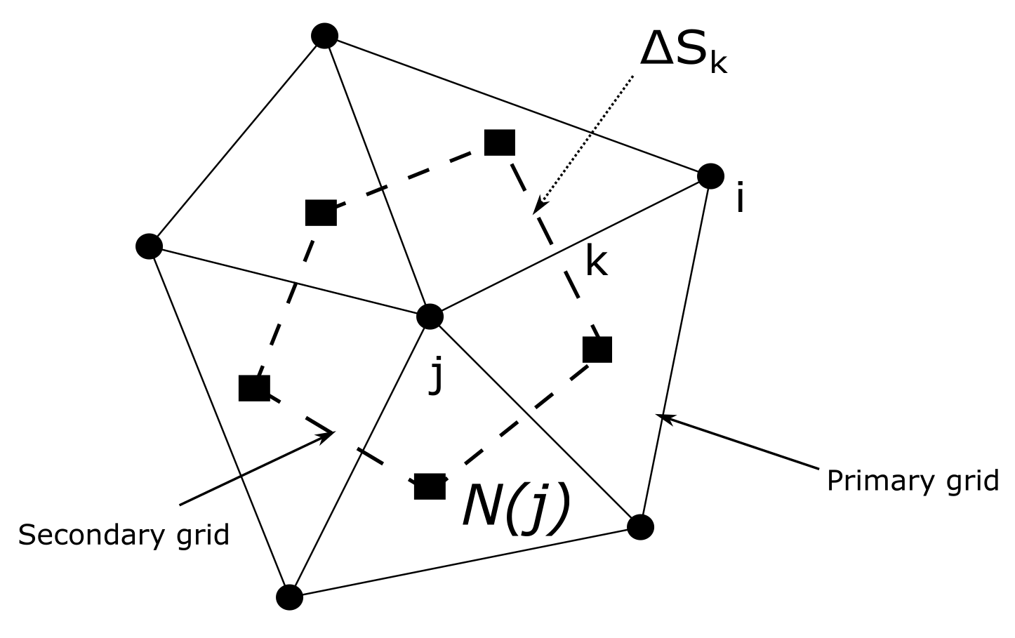
6.1. Solution Methodology

The compressible solver namely “RANS” available in SU2 is adopted in the present computations. Several validation studies of SU2 at high Mach numbers and at transonic conditions are available [8].

On the other hand, few low-Mach applications of incompressible SU2 solver are available [21]. As recommended from the developers’ community, SU2 is mainly developed for compressible applications. Therefore, rather than using the incompressible solver, the additional overhead represented by the slow convergence of a compressible solver at low-Mach is considered acceptable.

Furthermore, the preconditioning properties adopted in SU2 implementations allow for addressing the stiffness of low-Mach computations [22,23]. Convergence is assessed checking that the drop of $L_2$-norm of density residuals is at least $O\left({10}^{-6}\right)$. Convergence of aerodynamic coefficient is also monitored and simulation is stopped when maximum variation of coefficients over a specified iterations number is less than $0.1\%$ of its average value.

6.2. Numerical Schemes Adopted

Convective and diffusive fluxes are discretized with a second order accuracy in space, and gradients are evaluated with weighted least square schemes. Both second order central and upwind discretisations with MUSCL reconstruction are adopted for convective term discretisations [24,25].

Accordingly, numerical flux functions are evaluated at cell faces using the cell average values (which are second order accurate). The ROE scheme and JST scheme are adopted to discretise convective terms. In

Table 3. Effect of numerical discretization of convective terms $\alpha =8.{36}^{\circ }$.

Numerical Scheme	MUSCL	Limiter	${\mathit{ϵ}}_1$	${\mathit{ϵ}}_2$	${\mathit{C}}_{\mathit{L}}$	${\mathit{C}}_{\mathit{D}}$	Converged	${\mathit{C}}_{\mathit{L}}^{\mathit{exp}}$	${\mathit{C}}_{\mathit{D}}^{\mathit{exp}}$
ROE (2nd ord)	YES	Venkatakrishnan	-	-	0.45	0.045	YES	0.442	0.024
JST (2nd ord)	YES	Venkatakrishnan	0.5	0.02	0.43	0.031	YES	0.442	0.024
JST (2nd ord)	YES	Venkatakrishnan	0.38	0.01	0.42	0.029	YES	0.442	0.024
JST (2nd ord)	YES	Venkatakrishnan	0.36	0.01	-	-	NO	0.442	0.024

, comparisons of aerodynamic coefficients at $\alpha =8.{36}^{\circ }$ and experimental open tunnel data are shown. The use of a flux limiter is also adopted in the current computations to preserve monotonicity of solution at low-Mach conditions for the ROE scheme. The ROE scheme provides good estimation for the lift coefficient, while it clearly overshoots the drag coefficient. Because the JST scheme allows more accurate predictions of drag coefficient, the JST scheme is adopted in all following computations. It is worth noting that JST is also recommended by SU2 developers for some low-Mach applications for scale resolving simulations [22,24].

As expected, the drag coefficient is sensitive to JST coefficients ${ϵ}_1,{ϵ}_2$ i.e., (2nd and 4th order dissipation). The dissipation is triggered by a pressure sensor, which optionally activates the damping of spurious oscillations arising near shock waves. As in the present computations, no compressibility effects are involved, and ${ϵ}_1$ and ${ϵ}_2$ can be reduced to control numerical dissipation, thus improving drag computations (see Table 3). However, for ${ϵ}_1\le 0.36$, simulation becomes unstable as the numerical transient is not able to describe the pressure waves propagation in the low-Mach limit (the acoustic wave-speed order of magnitude being higher with respect to convective velocity). Therefore, numerical instabilities due to spurious modes arise and become not sufficiently damped by the second order dissipation.

In Table 3, a difference of 50 drag counts for the best settings of JST coefficients with respect to experimental data is observed. It is worth noting that such behaviour has been previously documented for RANS application of subsonic flow [24]. However, further reduction of 2nd order dissipation leads to an unstable simulation, such an issue being probably related to the adopted grid resolution. Although the actual grid resolution is finer than the one used in [6], eventually it requires a further refinement to resolve all the smallest numerical components of the solution, up to the Nyquist cut-off frequency, to avoid numerical instabilities arising on higher order terms of local truncation error.

7. Result Discussions with Experimental Data Comparisons

In this section, longitudinal aerodynamic coefficients (i.e., lift, drag, and pitching moment coefficients), as well as pressure distributions at four spanwise locations, namely $\beta =13.4\%$; $\beta =30.5\%$; $\beta =51.0\%$; $\beta =90.6\%$ according to Figure 8, are shown and discussed.

When available, experimental data are also provided and compared with outcomes of present numerical computations in order to address results’ reliability. The trend of aerodynamic coefficients related to flight attitudes is shown in Table 1, discussed considering the flow behaviour on the leeward surface.

Results are compared to low-subsonic numerical and experimental data collected for the N2A aeroshape, as hereinafter discussed [6,14,15,16]. To further support comparisons with experimental data, streamlines and skin-friction lines over BWB at different AoAs are also provided.

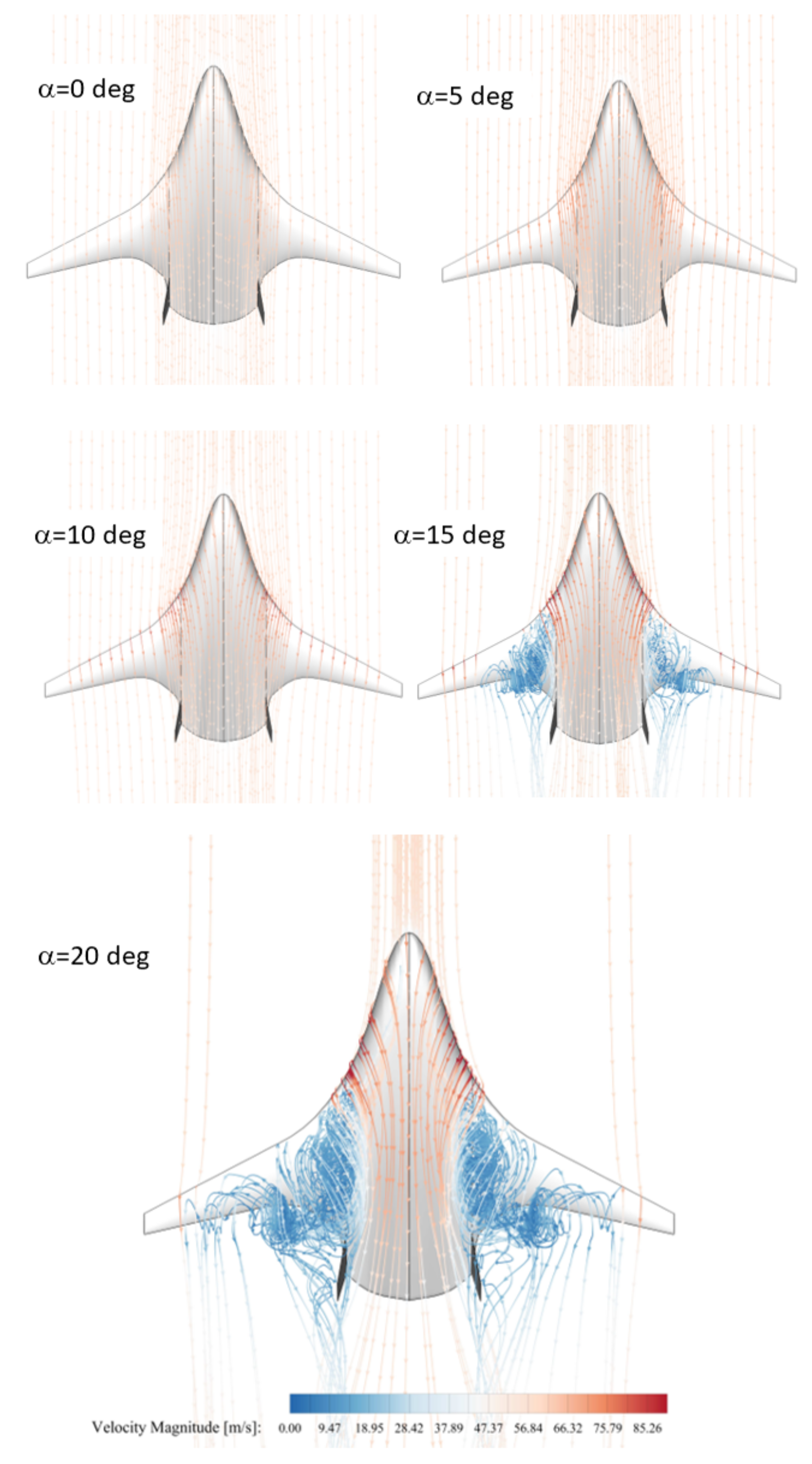
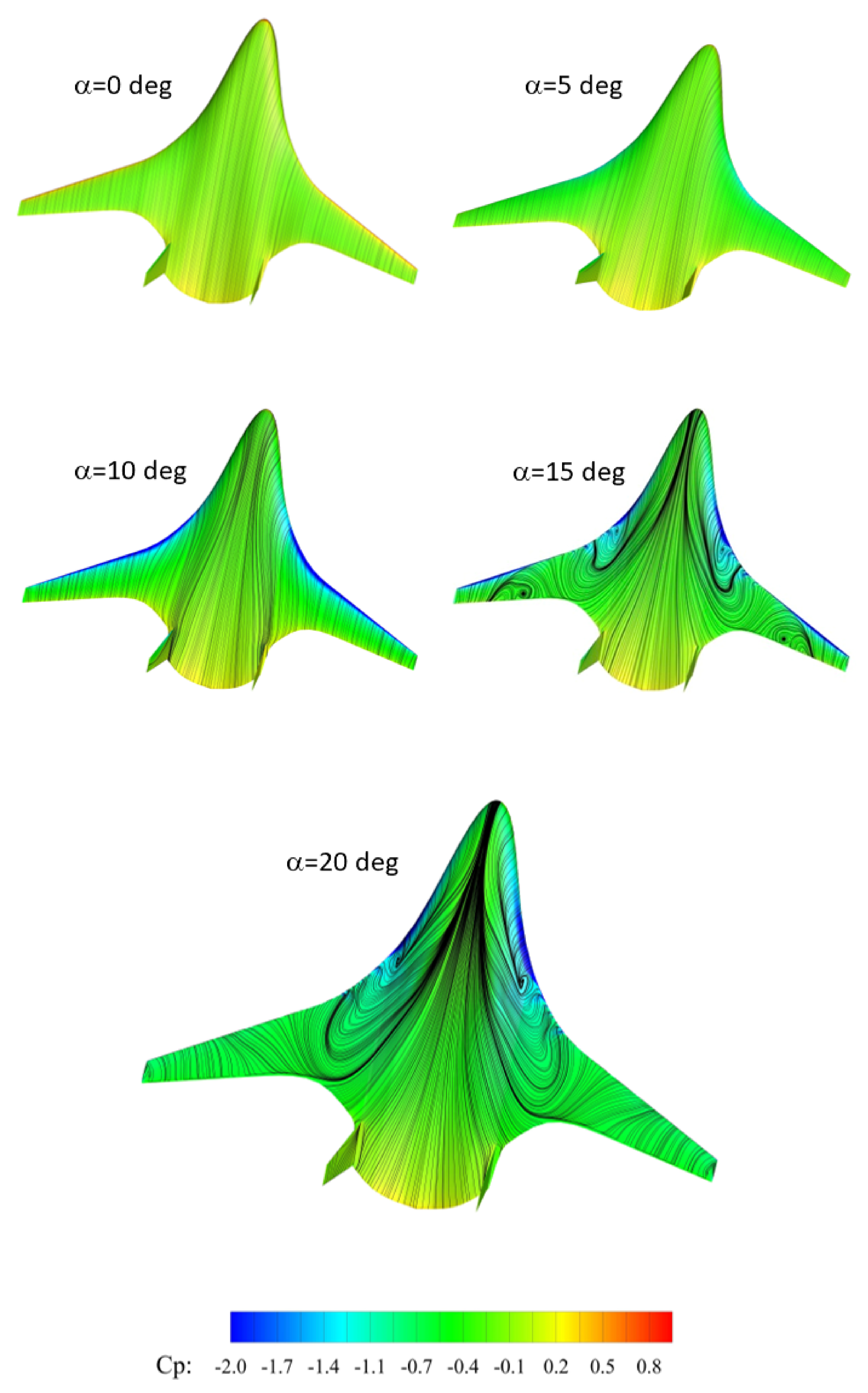
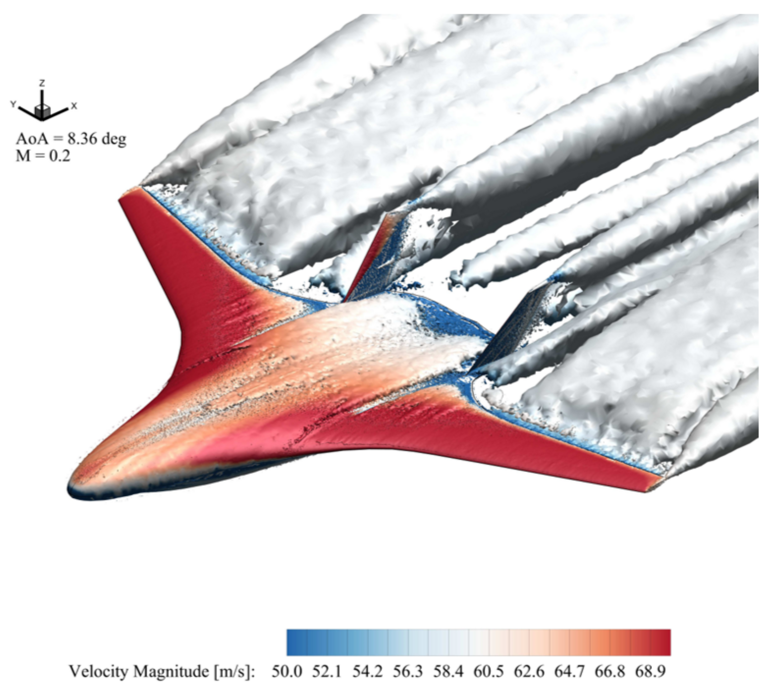
7.1. Flowfield Visualisation

In Figure 9, it is shown that an attached flow is observed up to ${10}^{\circ }$, as it is demonstrated by the ordered and very regular streamlines pattern.

A leading edge vortex emanates from the inboard region of the wing and rolls up at about $\alpha ={10}^{\circ }$ [26]. Leading edge vortex location is observed in Figure 10, where skin-friction lines scrubbing over the leeside are computed at $\alpha =$ $0^{\circ }$, $5^{\circ }$, ${10}^{\circ }$, and ${15}^{\circ }$.

By increasing the AoA from $\alpha ={10}^{\circ }$ to $\alpha ={15}^{\circ }$, the leading edge vortex bursts and breakdown location moves forward to the leading edge. For $\alpha \ge {10}^{\circ }$, surface flow visualization points out many areas of separated and reversed flow. At $\alpha ={15}^{\circ }$, the attached flow region is limited to the centerbody region and partially to wing tips (see Figure 9). The above observations agree well with experimental findings shown in [16], and it is explained considering that the flow at the wingtip is still attached because of the washout. At $\alpha ={20}^{\circ }$, two counter-rotating recirculating flow regions are shown on the aircraft leeward. One originates at the leading edge and extends up to the vertical tail (see Figure 9). The other starts on the rear part of the wing. In those regions, flow is fully three-dimensional and separated. The onset of flow-breakdown and the subsequent flow separation is further propagated downstream up to the trailing edge. This behaviour is also observed in experimental observations in [14], thus suggesting undesired loss of efficiency of the vertical tail.

To provide a further insight on the aerodynamic behaviour of the aeroshape at pre-stall AoAs, the mean-flow velocity field is computed at $\alpha =8.{36}^{\circ }$, and results are shown in Figure 11. For a steady flow field simulation (time averaged), a definition of a coherent structure cannot be applied. Therefore, detection criteria for a vortex structure are not significant. However, Q-criterion allows for detecting a greater order of magnitude of the rotational component of the mean flow field over its strain rate component, which is demonstrated by the current visualization. Therefore, it helps to detect regions where three-dimensional behaviour is broken (e.g., leading edge regions or wing tips). There, unsteady flow phenomena take place and lead to further involvement of aircraft i.e., vertical tail, which need further investigation with other levels of details.

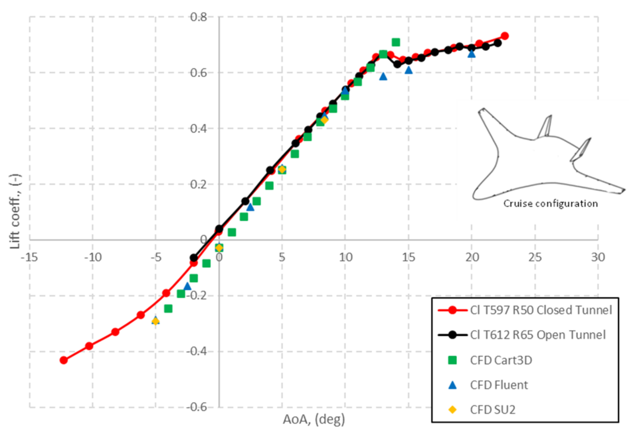
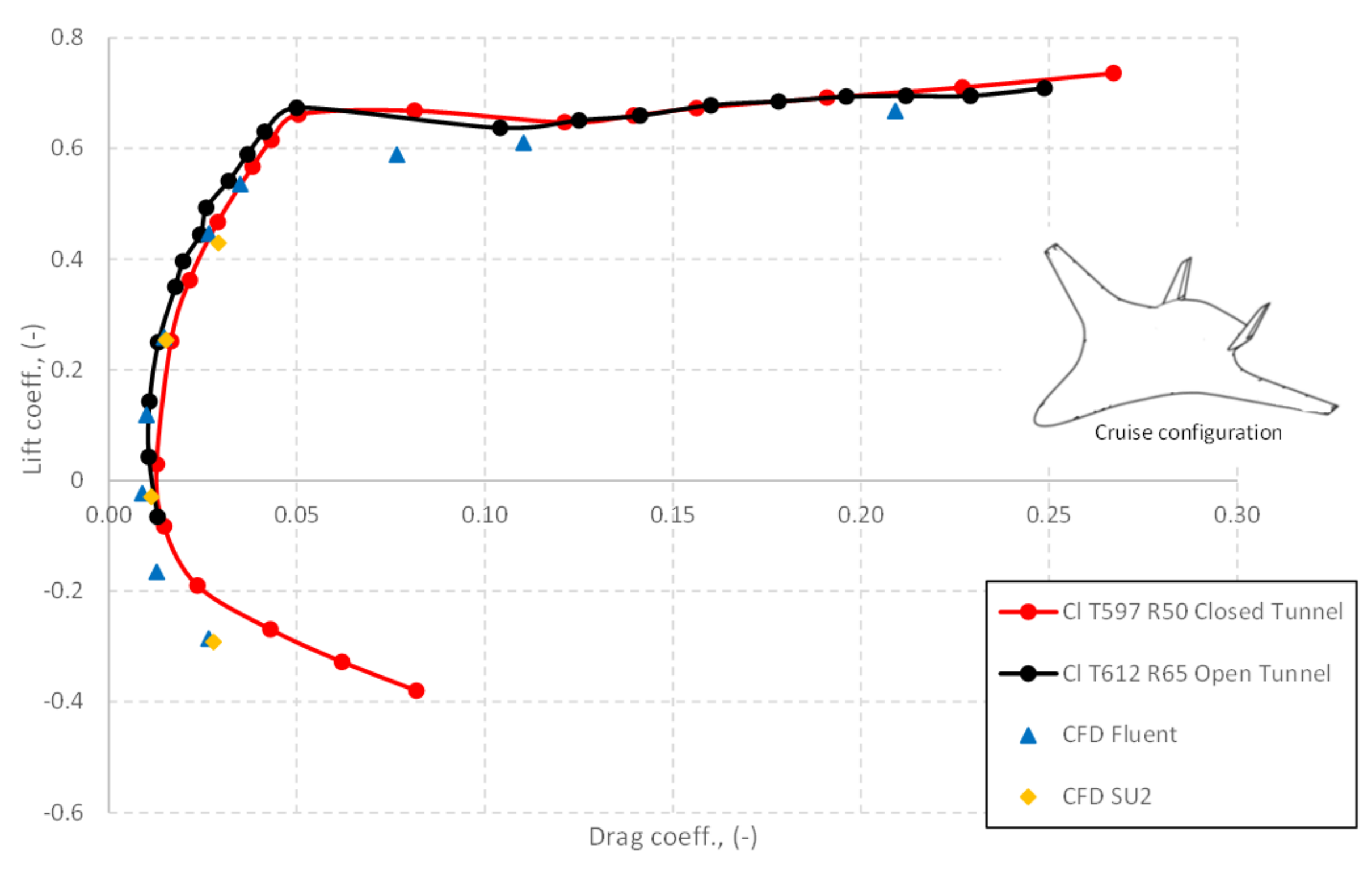
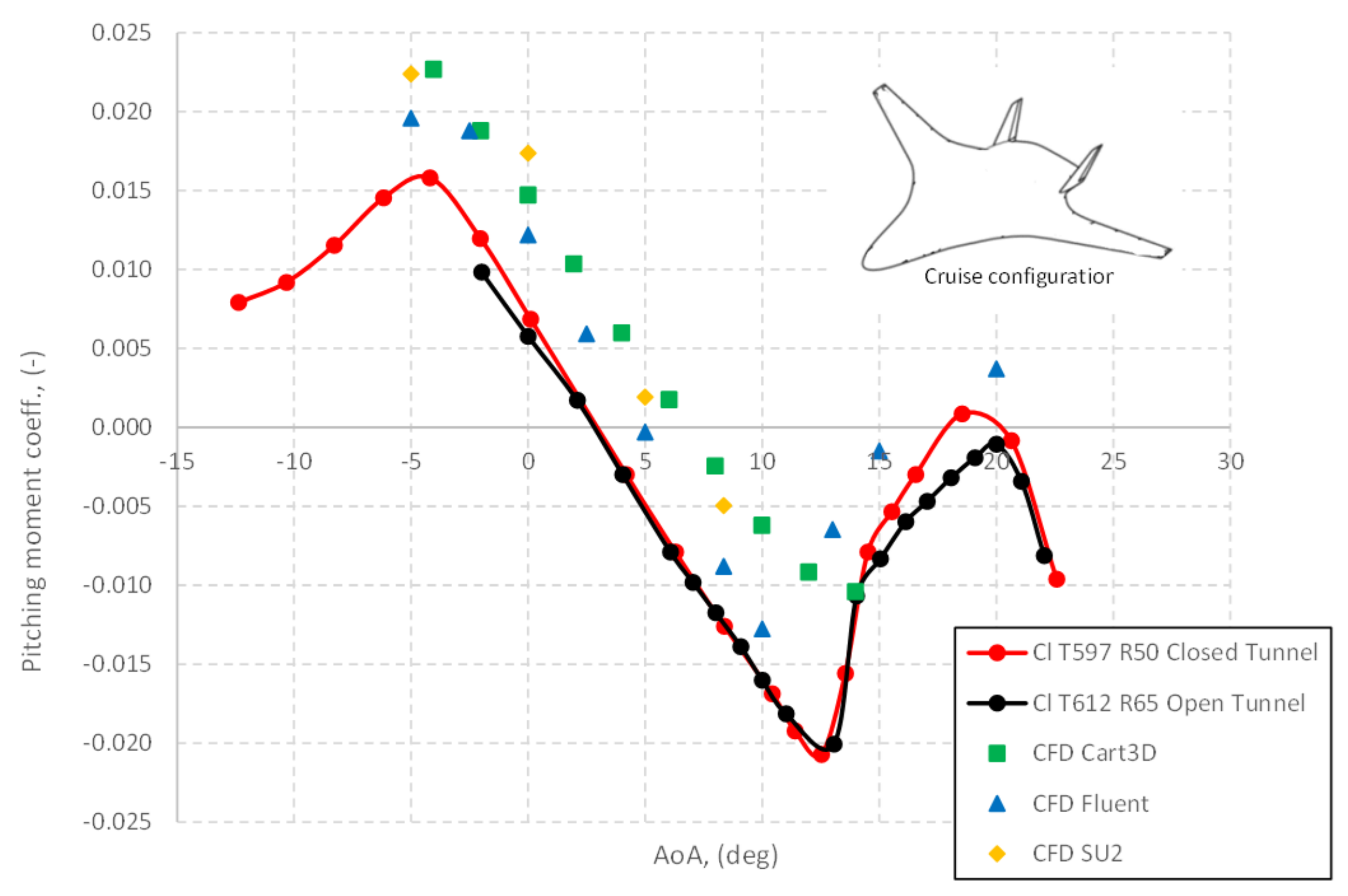
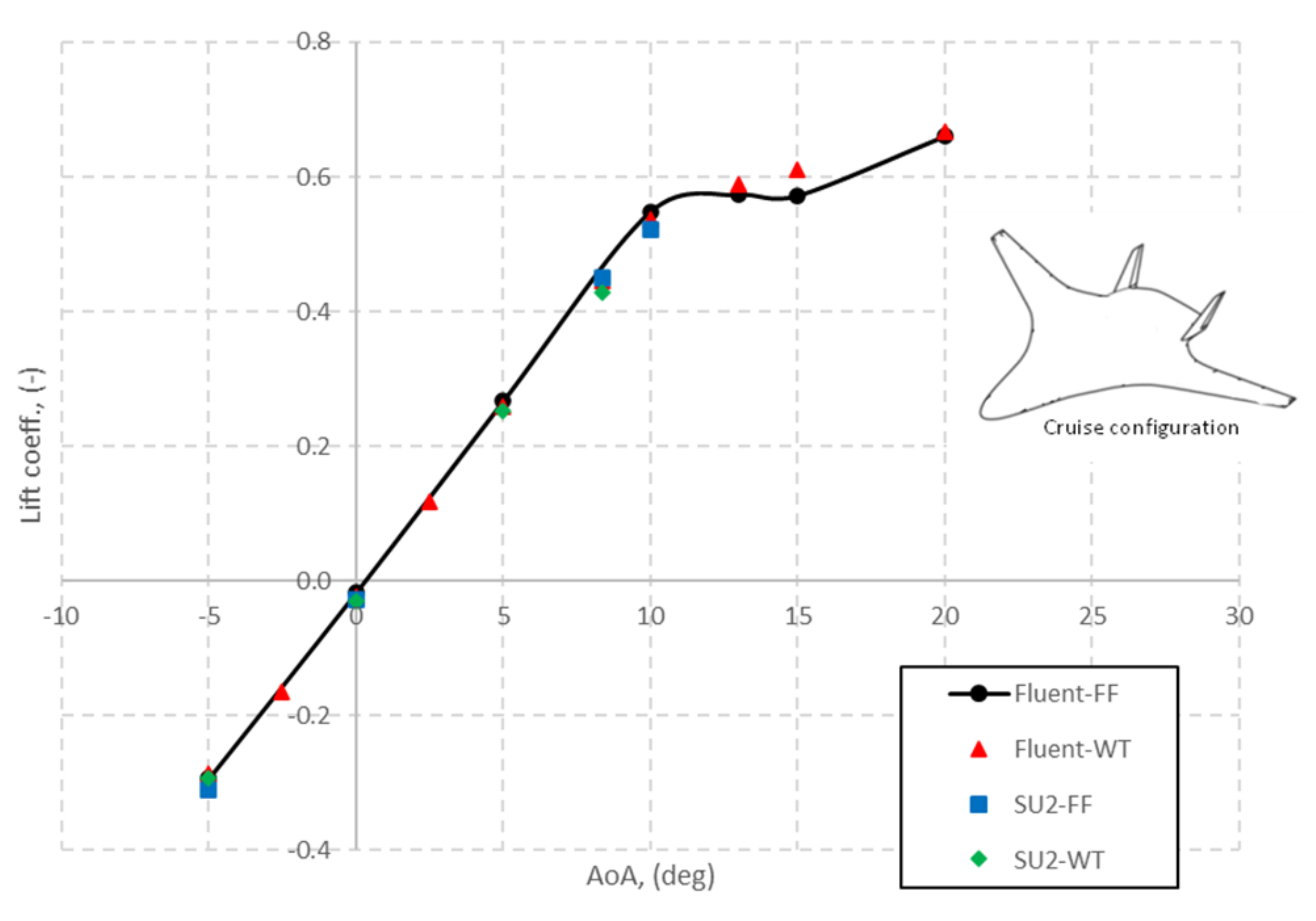
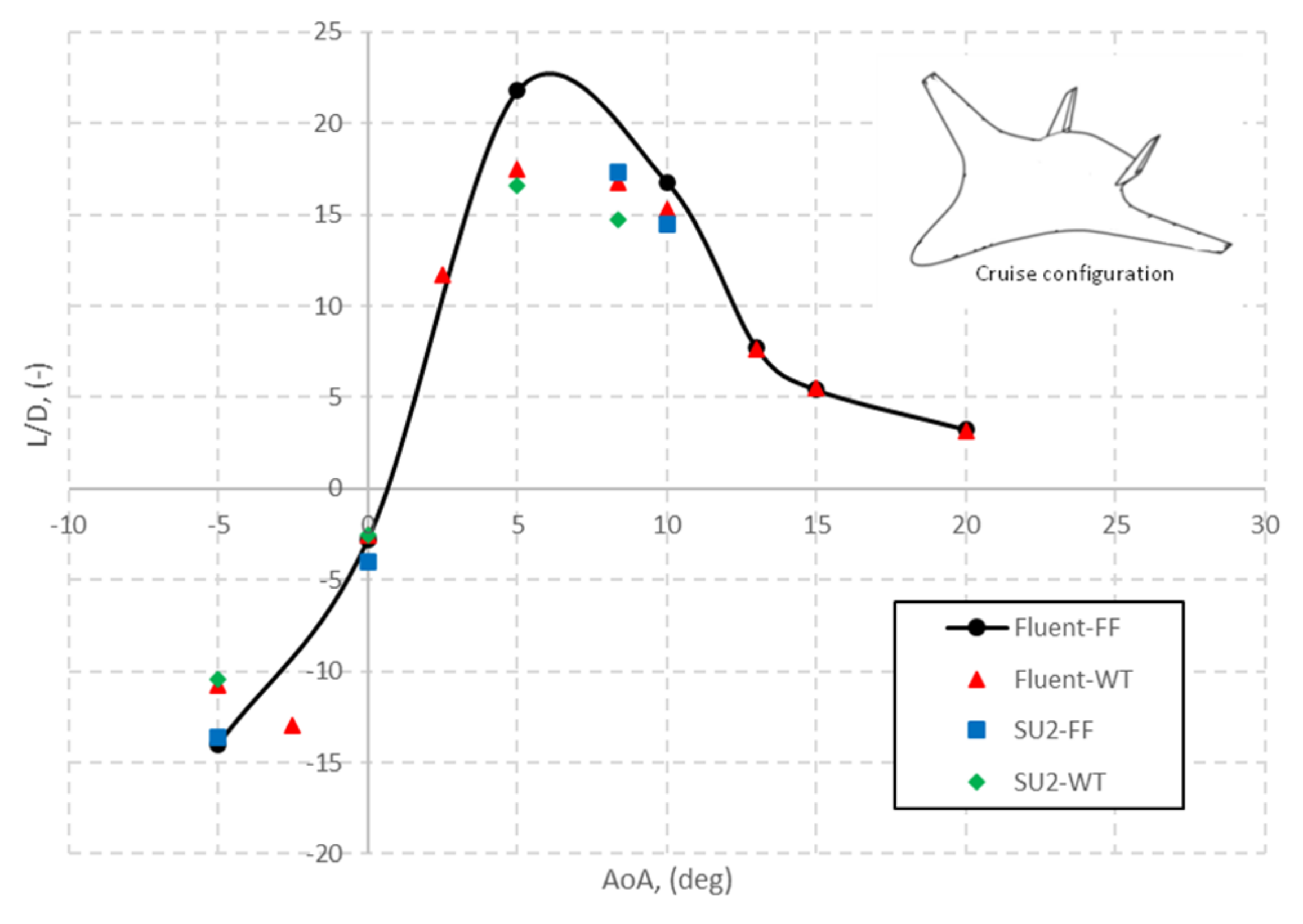
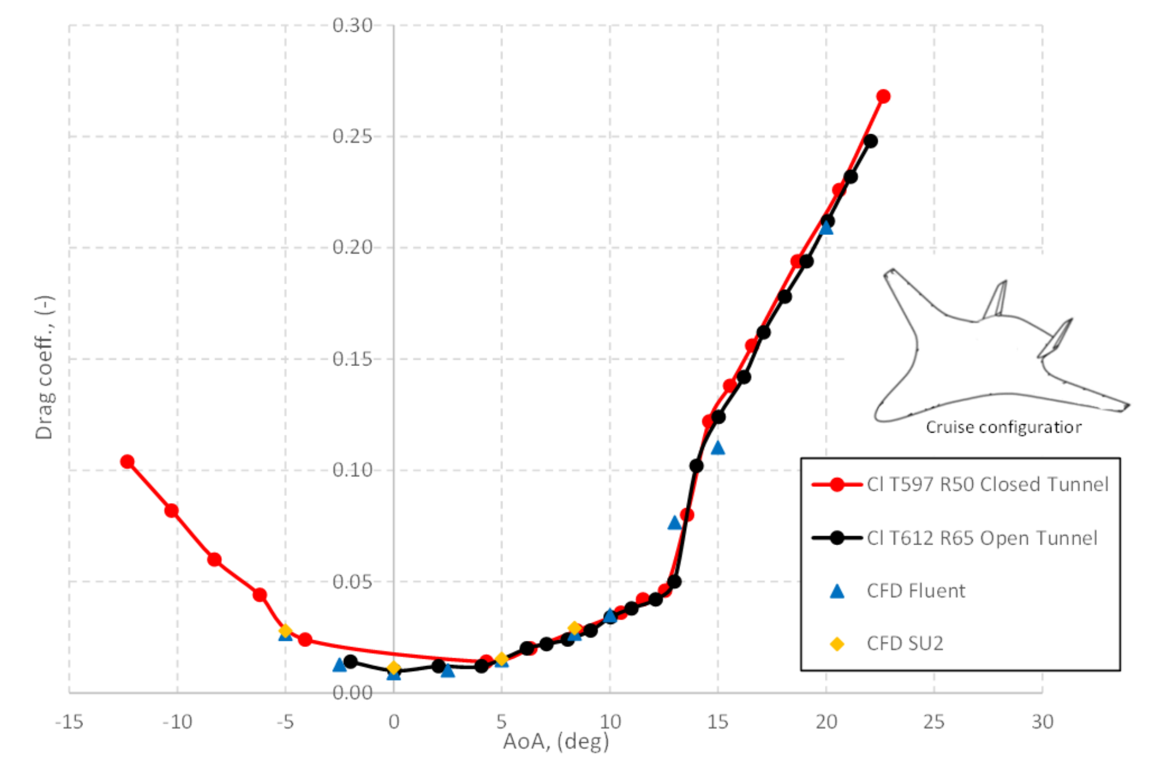
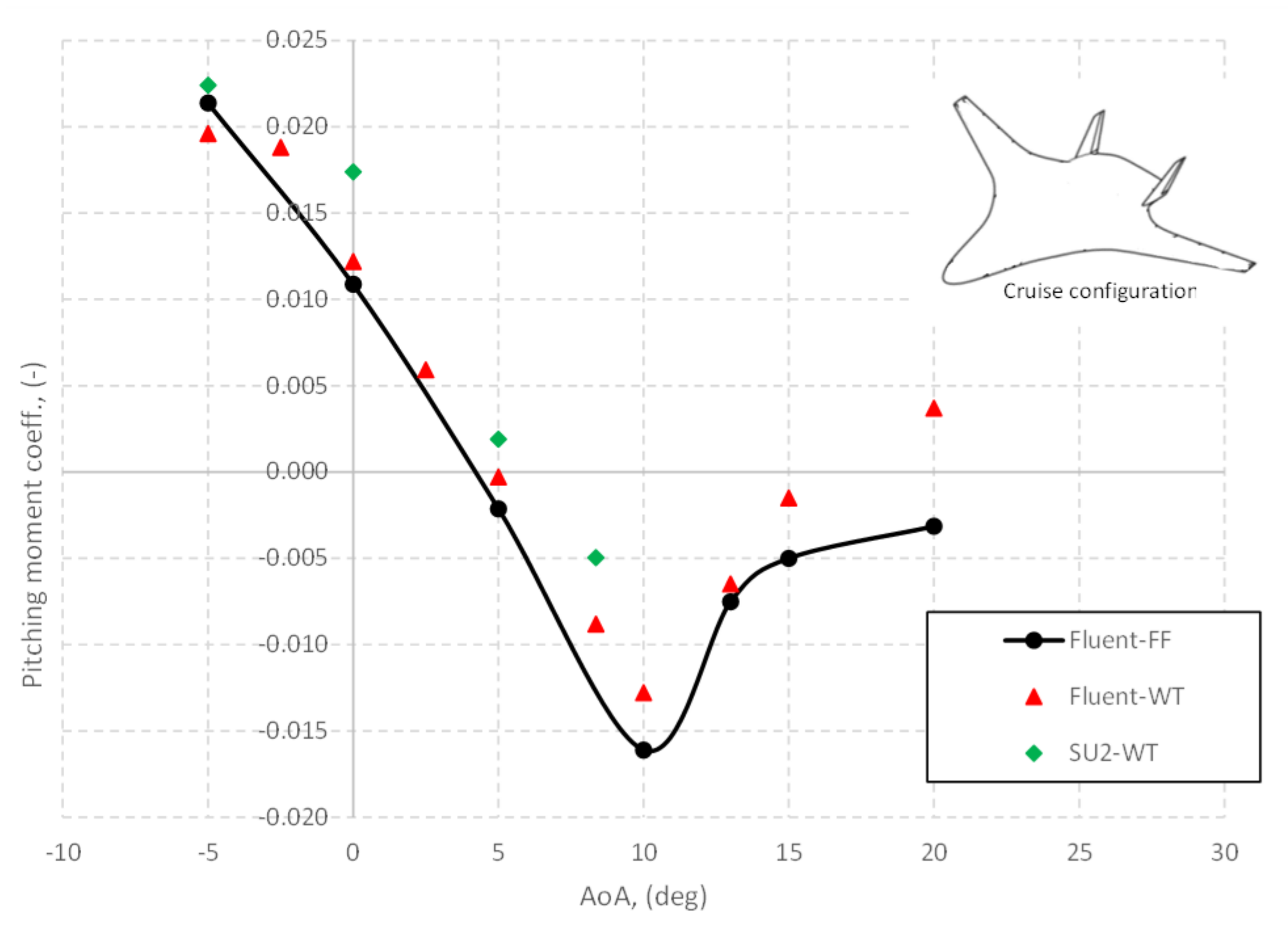
7.2. Aerodynamic Coefficients

In Figure 12, Figure 13, Figure 14 and Figure 15, aerodynamic coefficients versus AoA and drag polar are shown and compared to available WT data both for open (i.e., T612) and closed (i.e., T597) test sections. CFD predictions (i.e., Euler Cart3D) provided in Ref. [6] are also shown for further comparisons.

As it is shown in Figure 12, the lift coefficient exhibits a linear trend for flow incidences ranging from about $-5^{\circ }$ to ${13}^{\circ }$. Outside this attitude interval, significant changes of flow topology due to the onset of stall apply. A rather good prediction of lift coefficient is obtained for both the CFD tools adopted.

Specifically, CFD predictions fit very accurately experimental data immediately in pre-stall AoA. Additionally, both Fluent and SU2 follow the experimental lift slope also at negative AoAs, thus agreeing also with CART3D results. Post stall AoAs are characterized by an under prediction of the lift coefficient, which is due to inability of RANS simulation to describe three-dimensional instabilities and flow separation. Additionally, according to Ref. [6], discrepancies between WT and CFD data at small negative incidences ($0^{\circ }$ to $-5^{\circ }$) can be explained by recalling the wing washout (wing twist of $-8.{87}^{\circ }$ at tip) and the wing thickness taper. Therefore, when the aircraft is at $\alpha =-5^{\circ }$, this means that the effective AoA of the wingtip is $-13.{87}^{\circ }$. Therefore, a separation bubble is created on the wingtip. As far as AoA is increased, the bubble extends toward the inner body.

Conversely, CFD results provide a linear trend, suggesting that an attached flow condition is predicted [6]. Furthermore, experimental data in Figure 16 highlight a flow deceleration at the aircraft windside, which is opposite to the CFD results. This helps with explaining the mismatch between WT and CFD lift coefficient at pre-stall conditions, considering the pressure increase detected by WT data.

Looking at Figure 13, the drag coefficient also appears to be correctly computed except at low AoA, where an undershoot of $C_D$ is observed.

However, as friction drag contribution is an order of magnitude lower than induced drag, it appears that low-AoA undershoots can be possibly related to insufficient grid resolution. At higher AoA, the drag coefficient is better predicted. Post-stall evaluations reflect the well-known inability of RANS to predict flow instabilities and separation.

The same considerations apply for $C_L=C_L\left(C_D\right)$ where low-AoA drag undershoots are more clearly discernible. As confirmed from both the adopted CFD tools, grid resolution has a significant impact on convergence of results at low AoA [6].

The pitching moment coefficient versus AoA is provided in Figure 15. As it is shown, the behaviour of $C_{M_y}$ reflects the longitudinal stability trend depicted by experimental data, but with a nearly constant displacement of about $\Delta C_{M_y}=0.005$.

The shift between results of present numerical investigations and WT data could be probably due to the mismatch existing between numerical and WT lift coefficients (see Figure 12) that, according to Ref. [6], could be the result of interference from the support system used in the WT test campaigns. In fact, the increase in the pressure distribution on the aircraft windside in Figure 16 highlights a deceleration of the flow toward the center of the body. A little contribution of drag coefficient must be considered as well.

Furthermore, another contribution to this $C_{M_y}$ mismatch can be found by recalling that WT data are obtained also accounting for two flow-through nacelles, not included in the present CFD investigations.

Moreover, remarkable differences are found close to stall conditions (i.e., $\alpha ={13}^{\circ }$), thus highlighting that Fluent results at stall and post stall conditions do not feature good convergence for this HWB aeroshape. However, it is worth noting that, at $\alpha =5^{\circ }$, both CFD tools do not match the experimental stability behaviour.

Specifically, SU2 gives a longitudinally unstable behaviour, while FLUENT depicts a neutrally stable configuration.

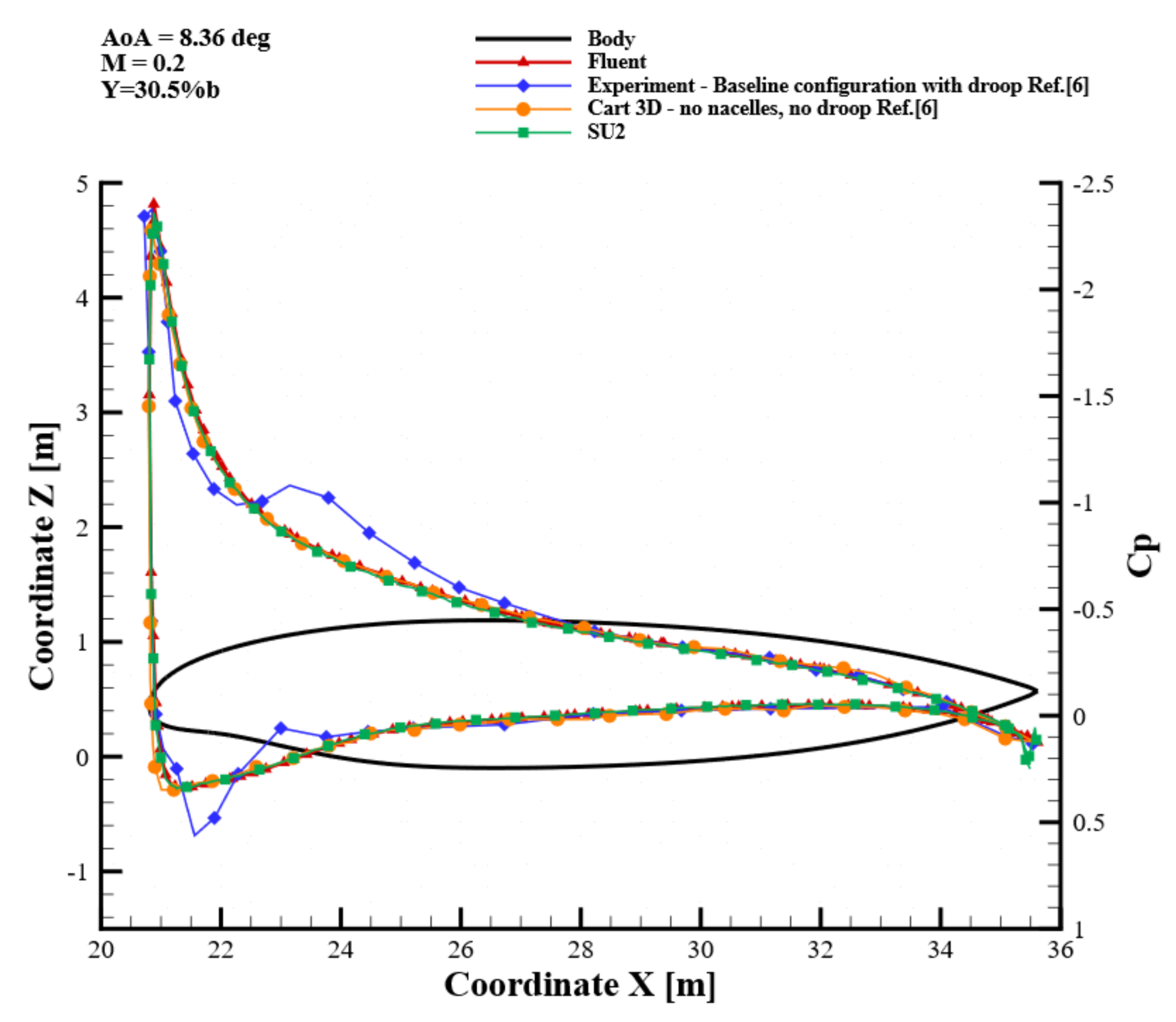
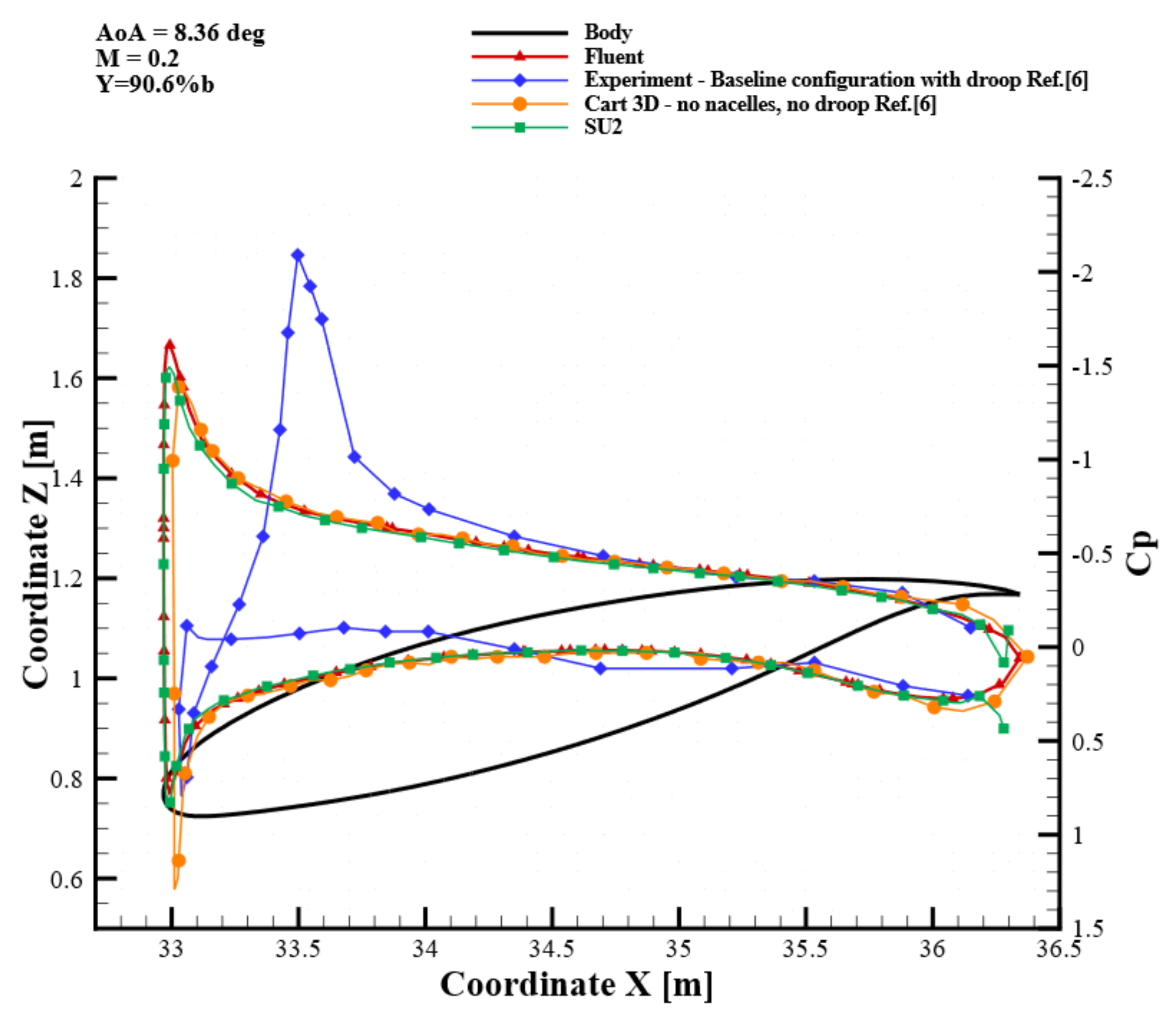
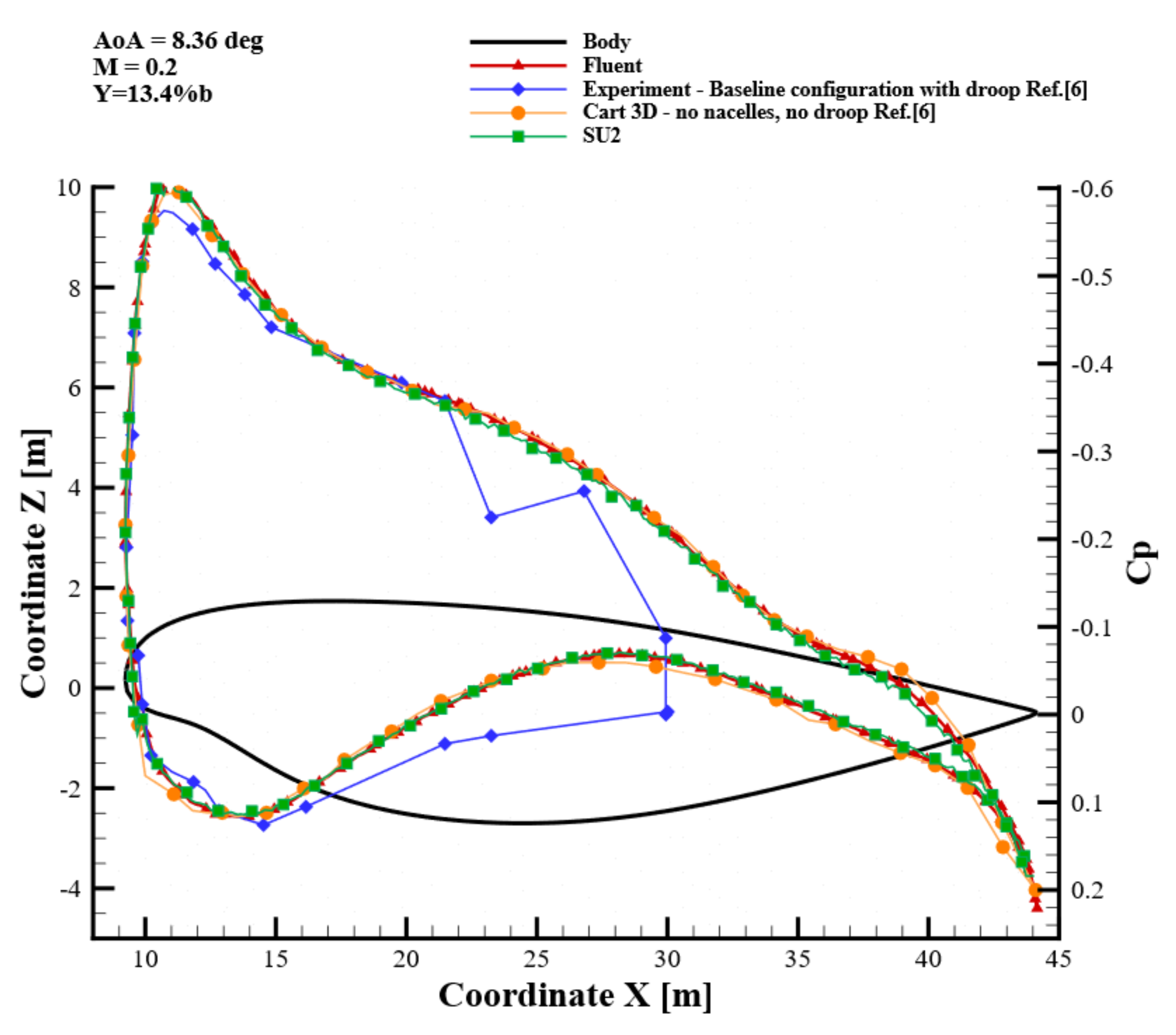
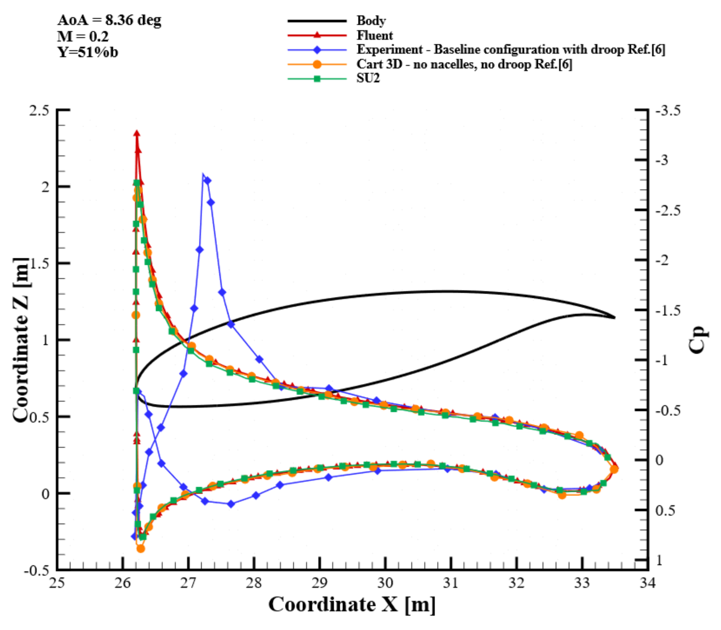
7.3. Pressure Coefficient Distributions

Pressure distributions computed with CFD simulation at four spanwise locations i.e., $13.4\%$, $30.5\%$, $51.0\%$, and $90.6\%$ annotated in Figure 8, are respectively shown in Figure 16, Figure 17, Figure 18 and Figure 19. To correctly ascertain comparisons between experimental and numerical results, it is worth noting that WT measurements refer to baseline configuration (i.e., model with dropped leading edge and nacelles), while CFD results are obtained on configuration without dropped leading edge and nacelles.

Although the simulated model refers to a watertight configuration (without leading edge droop and nacelles), the available experimental data were, to the best of the author’s knowledge, the only available in literature for comparisons. Furthermore, considering that the experimental results felt the presence of droop at $30.5\%$ and $51.0\%$ of spanwise location, leaving unaltered the pressure distribution over the trailing edge, a comparison with the simulated model (without droop and nacelles) can be performed.

In Figure 16, Figure 17, Figure 18 and Figure 19, it is shown that pressure coefficient is well predicted moving from the center body to the aircraft wingtips. Thus, CFD predicts well both the correct location and amplitude of expansion peak, and it is interesting to note that also simulation performed with CART3D behaves very similarly [6]. At spanwise location equal to $13.4\%$, the effect of the droop is not felt (see Figure 16).

Therefore, a good agreement with experimental data is observed at the leading edge. However, considering the pressure probe sections at $51.0\%$ and at $90.3\%$ (see Figure 18 and Figure 19), discrepancies between the simulated model and experimental data on the leading edge are observed because of the pressure spike induced by the droop [6]. Behind the induced-by-droop expansion, both FLUENT and SU2 results agree with experimental available data and with CART3D data as the effect of the droop progressively vanishes.

7.4. Reynolds Number Effect on Aircraft Aerodynamic Coefficients

According to Table 1, two flight conditions have been considered in addressing aircraft aerodynamics, namely WT test (i.e., $R{e}_{L_{ref}}=6.60\times {10}^6$) and free-flight (FF) (i.e., $R{e}_{L_{ref}}=1.27\times {10}^8$) conditions. The former Reynolds refers to testing the campaigns carried out in the NASA Langley 14-by-22 foot subsonic tunnel with a 5.8% scale model of N2A aircraft at $M_{\infty }=0.2$. Therefore, to properly model the effects of the viscous forces relative to the inertial ones, more realistic flight conditions must be considered for $M_{\infty }=0.2$. Thus, the $R{e}_{L_{ref}}=1.27\times {10}^8$ has been considered that corresponds to a full scale N2A aircraft flying at about 30 m altitude and 70 m/s speed. The effects of Reynolds number on aircraft aerodynamics are summarized from Figure 20, Figure 21, Figure 22 and Figure 23, where lift, drag, pitching moment coefficients and lift-to-drag ration are provided, respectively. In these figures, both Fluent and SU2 results are compared.

As shown, there is no significant effect of $Re$ on the lift coefficient characteristics in terms of strength to stall, while lower drag is detected at a higher Reynolds number, as expected. Drag counts difference between WT and FF are summarized in

Table 4. Reynolds number effect over drag coefficient.

AoA, deg	${\mathit{C}}_{\mathit{D}}\left(\mathit{WT}\right)$	${\mathit{C}}_{\mathit{D}}\left(\mathit{FF}\right)$	$\mathbf{\Delta }{\mathit{C}}_{\mathit{D}}$, Counts
−5	0.02655	0.0209	56.3
0	0.00896	0.0062	27.4
5	0.01476	0.0122	25.1
10	0.03497	0.0326	23.5
13	0.07666	0.0744	23.0
15	0.11031	0.1057	46.3
20	0.20918	0.2042	49.9

.

As far as the pitching moment is concerned, Figure 22 points out that the increase in Reynolds number does not affect aircraft static stability significantly; while the natural trim point lowers to about $\alpha =4$ deg, this means a $L/D$ decrease close to $10\%$, see Figure 23.

Finally, Figure 23 points out that a larger aerodynamic efficiency at FF conditions is expected. Specifically, L/D in FF is about $30\%$ and $13\%$ larger at $\alpha =5^{\circ }$ and $\alpha ={10}^{\circ }$, respectively.

8. Conclusions

Low-Mach number aerodynamic assessments of the non-proprietary N2A aeroshape has been addressed as a preparatory study phase to multidisciplinary design optimization procedures involving massive use of computational fluid dynamics. N2A is a hybrid wing–body twin-jet aircraft developed by NASA to study innovative aeroshape configurations capable of meeting low-noise and low-fuel burn requirements. Numerical investigations performed with two different CFD codes, namely Fluent and SU2 within pre-stall and attached flow conditions, were performed and compared with available literature data, both numerical and experimental. The largest outlier observed in numerical simulation is the pitching moment. A constant shift of $\Delta C{M}_y=0.005$ between the experimental and numerical data sets within the pre-stall conditions has been observed. Present results showed good agreement with the experimental measurements except at high incidence. In fact, predicting the separation as demonstrated by the under prediction of lift on a highly swept curved aeroshape, as the center body of N2A is a challenging problem for many CFD codes. Therefore, further investigations are mandatory and surely suggested. Although mean-flow evaluations were involved, current simulations demonstrated that, by increasing AoA, the inboard wing region, which has a larger leading edge radius, promotes vortex bursting and breakdown. The flow separation is not uniformly distributed over the blended wing body geometries. Vertical tails are also interested by the recirculating flow consequent to breakdown; therefore, more detailed unsteady studies are required.

Finally, considering the growing interest of research community around SU2, the current study demonstrates the robustness and accuracy of the present solver for future high-fidelity CFD data-driven conceptual designs.

References

1. Chen, Z.; Zhang, M.; Chen, Y.; Sang, W.; Tan, Z.; Li, D.; Zhang, B. Assesment on critical technologies for conceptual design of blended-wing-body civil aircraft. Chin. J. Aeronaut. 2019, 32, 1797–1827. [Google Scholar] [CrossRef]
2. Ikeda, T.; Bill, C. Aerodynamic performance of a Blended Wing Body Configuration Aircraft. In Proceedings of the International Congress of Aeronautical Sciences (ICAS), Hamburg, Germany, 3–8 September 2006. [Google Scholar]
3. Qin, N.; Vavalle, A.; Le Moigne, A.; Hackett, K.; Weinerfelt, P. Aerodynamic considerations of blended wing body aircraft. Prog. Aerosp. Sci. 2004, 40, 321–343. [Google Scholar] [CrossRef]
4. Lyu, Z.; Martins, J.R.R.A. Aerodynamic design optimization studies of a blended wing body aircraft. J. Aircr. 2014, 51, 1604–1617. [Google Scholar] [CrossRef] [Green Version]
5. Karpuk, S.; Yaolong, L.; Ehlam, A. Multi-fidelity design optimization of a Long-Range blended wing body aircraft with new aiframe technologies. Aerospace 2020, 7, 87. [Google Scholar] [CrossRef]
6. Almosnino, D. A Low Subsonic Study of the NASA N2A Hybrid Wing-Body Using an Inviscid Euler-Adjoint Solver. In Proceedings of the 34th Applied Aerodynamics Conference, Washington, DC, USA, 13–17 June 2016. [Google Scholar]
7. Aprovitola, A.; Iuspa, L.; Pezzella, G.; Viviani, A. Phase-A design of a reusable re-entry vehicle. Acta Astronaut. 2021, 187, 141–155. [Google Scholar] [CrossRef]
8. Economon, T.D.; Palacios, F.; Copeland, S.R.; Lukaczyk, T.W.; Alonso, J.J. SU2: An Open-SOurce suite for multiphysics simulation and design. AIAA J. 2016, 54, 828–846. [Google Scholar] [CrossRef]
9. Aprovitola, A.; Di Nuzzo, P.E.; Pezzella, G.; Viviani, A. Aerodynamic Analysis of a Supersonic Transport Aircraft at Landing Speed Conditions. Energies 2021, 14, 6615. [Google Scholar] [CrossRef]
10. Kontogianniss, A.; Parenteau, M. Viscous-Inviscid Analysis of Transonic Swept Wings using 2.5D RANS and Parametric Shapes. In Proceedings of the AIAA Scitech, San Diego, CA, USA, 7–11 January 2019. [Google Scholar]
11. Liebeck, R.H. Design of the blended wing body subsonic transport. J. Aircr. 2004, 41, 10–25. [Google Scholar] [CrossRef] [Green Version]
12. Liebeck, R.H.; Page, M.A.; Rawdon, B.K. Blended-wing-body subsonic commercial transport. In Proceedings of the 36th Aerospace Sciences Meeting & Exhibit, Reno, NV, USA, 12–15 January 1998. [Google Scholar]
13. Deere, K.A.; Luckring, J.M.; McMillin, S.N.; Flamm, J.D.; Roman, D. CFD predictions for transonic performance of the ERA hybrid wing-body configuration (invited). In Proceedings of the 54th AIAA Aerospace Sciences Meeting, San Diego, CA, USA, 4–8 January 2016. [Google Scholar]
14. Gatlin, G.M.; Vicroy, D.D.; Carter, M.B. Experimental Investigation of the Low-Speed Aerodynamic Characteristics of a 5.8-Percent Scale Hybrid Wing Body Configuration. In Proceedings of the 30th AIAA Applied Aerodynamics Conference, New Orleans, LA, USA, 25–28 June 2012; Volume 1. [Google Scholar]
15. Vicroy, D.D. Blended-Wing-Body Low-Speed Flight Dynamics: Summary of Ground Tests and Sample Results (Invited). In Proceedings of the 47th AIAA Aerospace Sciences Meeting and Exhibit, Orlando, FL, USA, 5–8 January 2009. [Google Scholar]
16. Vicroy, D.D.; Gatlin, G.M.; Jenkins, L.N.; Murphy, P.C.; Carter, M.B. Low-Speed Aerodynamic Investigations of a Hybrid Wing Body Configuration. In Proceedings of the 32th Applied Aerodynamics Conference, Atlanta, GA, USA, 16–20 June 2014. [Google Scholar]
17. NASA N2A Hybrid Wing Body. Available online: http://hangar.openvsp.org/vspfiles/349 (accessed on 1 December 2021).
18. Dowling, A.; Greitzer, E. The Silent Aircraft Initiative—Overview. In Proceedings of the 45th AIAA Aerospace Sciences Meeting and Exhibit, 2007-0452CP, Reno, NV, USA, 8–11 January 2006. [Google Scholar]
19. Ansys Fluent User’s Guide 2019R1; ANSYS, Inc.: Canonsburg, PA, USA, 2019.
20. Vitale, S.; Pini, M.; Colonna, P.; Gori, G.; Guardone, A.A.; Economon, T.D.; Palacios, F.; Alonso, J.J. Extension of the SU2 Open Source CFD code to the simulation of turbulent flows of fluids modelled with complex thermophysical laws. In Proceedings of the AIAA Aviation, Dallas, TX, USA, 22–26 June 2015. [Google Scholar]
21. Ravishanara, A.K.; Ozdemir, H.; van der Weide, E. Implementation of a pressure based incompressible flow solver in SU2 for wind turbine applications. In Proceedings of the AIAA Scitech, Orlando, FL, USA, 6–10 January 2020. [Google Scholar]
22. Molina, E.; Alonso, J.J. Scale-Resolving simulations in SU2. In Proceedings of the 1st SU2 Conference, Princeton, NJ, USA, 10–12 June 2020. [Google Scholar]
23. Duraisamy, K. Entropy-Stable Schemes in the Low-Mach-Number regime: Flux preconditioning, entropy breakdowns, and entropy transfers. arXiv 2021, arXiv:2110.11941. [Google Scholar]
24. SU2 Website Documentation. Available online: https://su2code.github.io (accessed on 21 December 2021).
25. Vleer, B. Towards the Ultimate Conservative Difference Scheme III. Upstream-centered Finite Difference Schemes for Ideal Compressible Flow. J. Comput. Phys. 1977, 23, 263–275. [Google Scholar]
26. Viviani, A.; Aprovitola, A.; Iuspa, L.; Pezzella, G. Low Speed Longitudinal Aerodynamics of a Blended Wing-Body Re-Entry Vehicle. Aerosp. Sci. Technol. 2020, 107, 106303. [Google Scholar] [CrossRef]
Figure 1. N2A aircraft aeroshape: realistic configuration (up); simulated configuration (down).
Aerospace 09 00089 g001
Figure 2. Three views drawing of N2A aircraft. Dimensions in metres.
Aerospace 09 00089 g002
Figure 3. Longitudinal aerodynamic coefficients according to ISO 1151 standard.
Aerospace 09 00089 g003
Figure 4. Computational domain brick with the details of the aircraft on its center.
Aerospace 09 00089 g004
Figure 5. Unstructured polyhedral grid on the aircraft longitudinal plane. Details of mesh close to the aircraft.
Aerospace 09 00089 g005
Figure 6. Unstructured triangular mesh on the airplane surface. Details of mesh on the portside of the left vertical tail.
Aerospace 09 00089 g006
Figure 7. Sketch of an edge-based dual grid control volume grid.
Aerospace 09 00089 g007
Figure 8. Locations of the four chordwise pressure tap rows on aircraft aeroshape.
Aerospace 09 00089 g008
Figure 9. Computed streamlines at α = 0 , 5 , 10 , 15 , 20 ; colour scale based on velocity magnitude.
Aerospace 09 00089 g009
Figure 10. Shearlines and pressure coefficient (Cp) distribution at different AoAs, namely 0 , 5 , 10 , 15 , and 20 .
Aerospace 09 00089 g010
Figure 11. Three dimensional visualization of mean flow field at α = 8 . 36 .
Aerospace 09 00089 g011
Figure 12. Lift coefficient. Comparison between present results and literature data [6,14,15,16].
Aerospace 09 00089 g012
Figure 13. Drag coefficient. Comparison between present results and literature data [6,14,15,16].
Aerospace 09 00089 g013
Figure 14. Drag polar. Comparison between present results and literature data [6,14,15,16].
Aerospace 09 00089 g014
Figure 15. Pitching moment coefficient. Comparison between present results and literature data [6,14,15,16].
Aerospace 09 00089 g015
Figure 16. Chordwise pressure distribution at β = 13.4 % . Comparison between present results and literature data.
Aerospace 09 00089 g016
Figure 17. Chordwise pressure distribution at β = 30.5 % , comparison between present results and literature data.
Aerospace 09 00089 g017
Figure 18. Chordwise pressure distribution at β = 51.0 % , comparison between present results and literature data.
Aerospace 09 00089 g018
Figure 19. Chordwise pressure distribution at β = 90.6 % , comparison between present results and literature data.
Aerospace 09 00089 g019
Figure 20. Lift coefficients versus AoA, effect of the Reynolds number.
Aerospace 09 00089 g020
Figure 21. Drag coefficients versus AoA, effect of the Reynolds number.
Aerospace 09 00089 g021
Figure 22. Pitching moment coefficients versus AoA, effect of Reynolds number.
Aerospace 09 00089 g022
Figure 23. Lift-to-drag ratio versus AoA, effect of Reynolds number.
Aerospace 09 00089 g023