Article

In-Situ Optical Measurements of Solid and Hybrid-Propellant Combustion Plumes

by
Stephen A. Whitmore
1,*,
Cara I. Frischkorn
1 and
Spencer J. Petersen
2
1
Department of Mechanical and Aerospace Engineering, Utah State University, Logan, UT 84322, USA
2
Department of Mechanical Engineering, Weber State University, Ogden, UT 84408, USA
*
Author to whom correspondence should be addressed.
Aerospace 2022, 9(2), 57; https://doi.org/10.3390/aerospace9020057
Submission received: 26 December 2021 / Revised: 17 January 2022 / Accepted: 18 January 2022 / Published: 23 January 2022
(This article belongs to the Special Issue Advances in Aerospace Sciences and Technology II)

Abstract

:
A method for in-situ optical measurements of solid and hybrid propellant rocket plumes is developed, and results from proof of concept tests are presented. The developed method inserts fiber-optic cables acting as radiation conduits into the solid-fuel combustion port, allowing optical signals to be transmitted from the flame zone to externally-mounted spectrometers. Multiple hot-firings using a using a lab-scale gaseous-oxygen, thermo-plastic fueled hybrid rocket system were performed to validate the sensing method. Burn durations varied from 5 to 25 s, and the inserted fiber optic sensors survived for all of the hot fire tests. The obtained optical spectra were curve-fit to Planck’s black-body radiation law, and Wien’s displacement law was used to estimate the internal flame-temperature. Optically-sensed flame-temperatures are correlated to analytical predictions, and shown to generally agree within a few degrees. Additionally, local maxima in the optical spectra are shown to correspond to emission frequencies of atomic and molecular hydrogen, water vapor, and molecular nitrogen; all species known to exist in the hybrid combustion plume. Based on these preliminary test results, it is concluded that this simple in-situ measurement system operates as designed, and it shows considerable promise for future applications to a wide swath of gas-generator systems.

1. Introduction

Due to the hostility of the combustion environment, obtaining in-situ thermal measurement of rocket plumes is an extremely difficult task. Currently the only feasible technique for collecting internal plume data involves the installation of Gardon heat-flux gauges [1]. Gardon gauges are capable of sensing very high radiative heat flux levels, but require a complex and invasive installation. A typical installation must install the sensor into a port in the motor case sidewall, with a sapphire optical window protecting the gauge from the high temperatures. Figure 1a shows a Schmidt-Boelter [2] type of gauge, with Figure 1b depicting a typical installation, and Figure 1c depicting typical heat flux paths. Water cooling is required. In Figure 1a the sensor body, quartz window, water cooling pipes, and mounting flange clearly visible. The optical window is subject to stress-fracture and is easily contaminated by the internal exhaust products. Gardon gauges cannot distinguish between convective and radiative heat flux. Finally, due to their intrusive nature, Gardon gauges cannot be used for fight applications.
This project investigates an alternative, minimally-intrusive approach for obtaining in-situ plume measurements. In this approach fiber optic cables are mounted between the motor case and the outer surface of the solid-fuel grain, and routed to look directly into the plume core flow. The cables transmit optical signals from the internal flame zone to externally-mounted spectrometers. Although the fiber optic cables inserted into the flow are consumed by the flame, the tips of the cables remain at the solid fuel boundary and recede at the same rate as the regressing fuel surface. Figure 2 shows results from an early proof-of-concept test; whereby, a fiber optic cable was mounted into ethylene propylene diene monomer (EPDM) rubber and burned using an oxy-acetylene torch. Figure 2c shows that the melted fiber optic tip still transmits light through the cable. Following each of the initial burn tests, the optical-response of the melted fiber-optic cable was compared to that of a fresh-cable using a known light source. The associated output spectra were essentially identical. Thus, it appears that the melted tip does not significantly distort the sensed spectrum.

2. Tests Systems

This section describes the test apparatus used for this development campaign. The fiber-optic sensor systems and the associated spectrometers will be described first. The hybrid rocket motor test systems, and their adaptations for fiber optic measurements will be presented next. Finally, the instrumentation systems used to collect the motor performance data will be described.

2.1. Optical Systems Design

For the testing campaign to be reported, two C11708MA [3] miniature spectrometers (Hamamatsu, city, country) were adapted as the optical sensors. The units were designed for installation into mobile measurement equipment and feature a complementary metal oxide semiconductor (CMOS) image sensor integrated with a light receiving slit and. The internal optical system is comprised of a convex lens with a grating etched by nano-imprint. These spectrometers have a nominal operating range that covers part of the visible and infrared spectra, from approximately 640 to 1050 nm wavelengths. Figure 3a shows the custom adapter designed connect the fiber optic cable to the spectrometer head. Figure 3b plots the response transfer function of the Hamamatsu spectrometers, and Figure 3c shows a schematic of the spectrometer processing system and acquisition systems.

2.2. Thrust Chamber Assembly

In order to test the fiber-optic systems in a realistic environment, a legacy 75-mm hybrid thruster system previously used by Whitmore et al. [4,5] for hydrogen peroxide testing was re-purposed to use gaseous oxygen (GOX) as the oxidizer. As a time and cost-saving measure for this study, 3-D printed and extruded acrylonitrile butadiene styrene (ABS) was used in lieu of hydroxyl-terminated polybutadiene as the fuel. Figure 4 shows the thrust chamber. Major system components are: (1) the nozzle assembly, (2) nozzle retention ring, (3) motor case, (4) 3D printed ABS ignitor cap with embedded electrodes, extruded main fuel grain section (5) insulating phenolic liner, (6) chamber pressure fitting, and (7) motor cap with a single-port injector. The 75-mm diameter motor case, constructed from 6061-T6 aluminum, was procured commercially. (Anon., “Cesaroni Pro-X, A Better Way to Fly, Pro75® hardware”, http://pro75.com/products/pro75/pro75.php, (accessed on 15 April 2020)). Full details of the motor systems are presented by Whitmore et al. [6].
Motor ignition relies on the patented low-wattage arc-ignition system invented at Utah State University (USU). [7] The fuel grain was fabricated in four pieces. The head-end section, depicted as the red segment in Figure 4, is manufactured from Stratasys ABSPlus-340 feed stock, (Anon., “ABSplus, For Mechanical Strength and Multi-Colors”, Stratasys Inc. Spec. Sheet, https://www.stratasys.com/materials/search/absplus (accessed on 25 July 2016)) printed at full in-fill density using a Stratasys Dimension ES-1200 FDM printer. (Anon., “Dimension 1200es, Durability Meets Affordability”, http://www.stratasys.com/3d-printers (accessed on 15 October 2021)) The head-end section has 3-D printed slots where the ignition electrodes are inserted. Printed inserts protect the embedded electrode wires from the combustion flame. Impingement shelves help to concentrate oxygen locally in the head end, facilitating ignition. Figure 4 also depicts the fiber optic cable routed through the injector cap, along the outer fuel grain wall and into the fuel port, and along the nozzle wall and into the fuel grain. The upper and lower sections of the fuel grain, pictured in blue in by Figure 4, were also 3-D printed from ABS Plus feedstock. The center section, pictured as light beige, was machined from a solid piece of extruded ABS, procured commercially. (Impact-Resistant Easy-to-Form ABS Rods, https://www.mcmaster.com/abs/shape~rod-and-disc/ (accessed on 15 October 2021)) This design allows optical plume sensing at two points along the fuel port. The extruded grain section has essentially the same thermodynamic properties as the printed section but can be procured at considerably less cost.

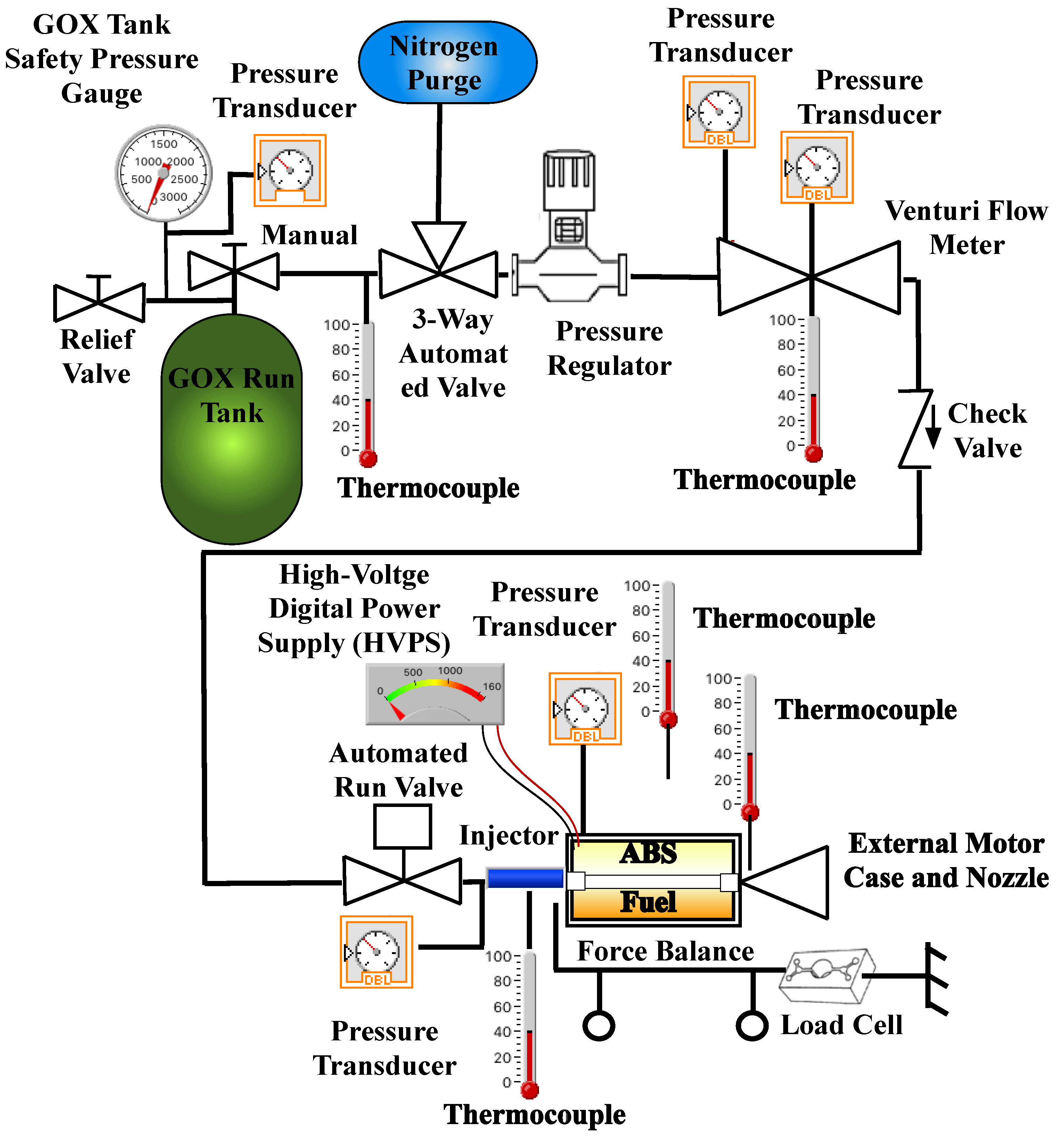
2.3. Motor Instrumentation and Test Assembly

Figure 5 shows the piping and instrumentation diagram (P&ID) of the experimental apparatus used for this test series. Test stand measurements include Venturi-based oxidizer mass flow, load-cell based thrust, chamber pressure, GOX tank pressure, injector feed pressure, and multiple thermocouples mounted at various points along the flow path. The motor was mounted to a custom-built and calibrated thrust-stand with flexible mounts that allowed thrust transmission in the axial direction. Also depicted by Figure 5 is the high voltage power system (HVPS) used for motor ignition. Custom fire control, data acquisition, and processing software were pre-programmed to ensure run-to-run test consistency. Connection from the motor instrumentation pallet to the control/data logging laptop was via a single universal serial bus (USB) cable. All tests to be reported were performed in the Battery and Survivability Limits Testing (BLAST) Lab on the USU campus. Separate laptops were used for motor performance and optical spectrum data logging.

3. Analytical Methods

This section details the theoretical and analytical methods that were essential to support the results of this study. A thermochemical analysis of the ABS fuel material and its combustion with gaseous oxygen is presented first. Methods used to reduce and interpret the motor performance data will be presented next. Finally, the methods used to interpret the plume spectra data and their correlations with the motor performance data will be presented.

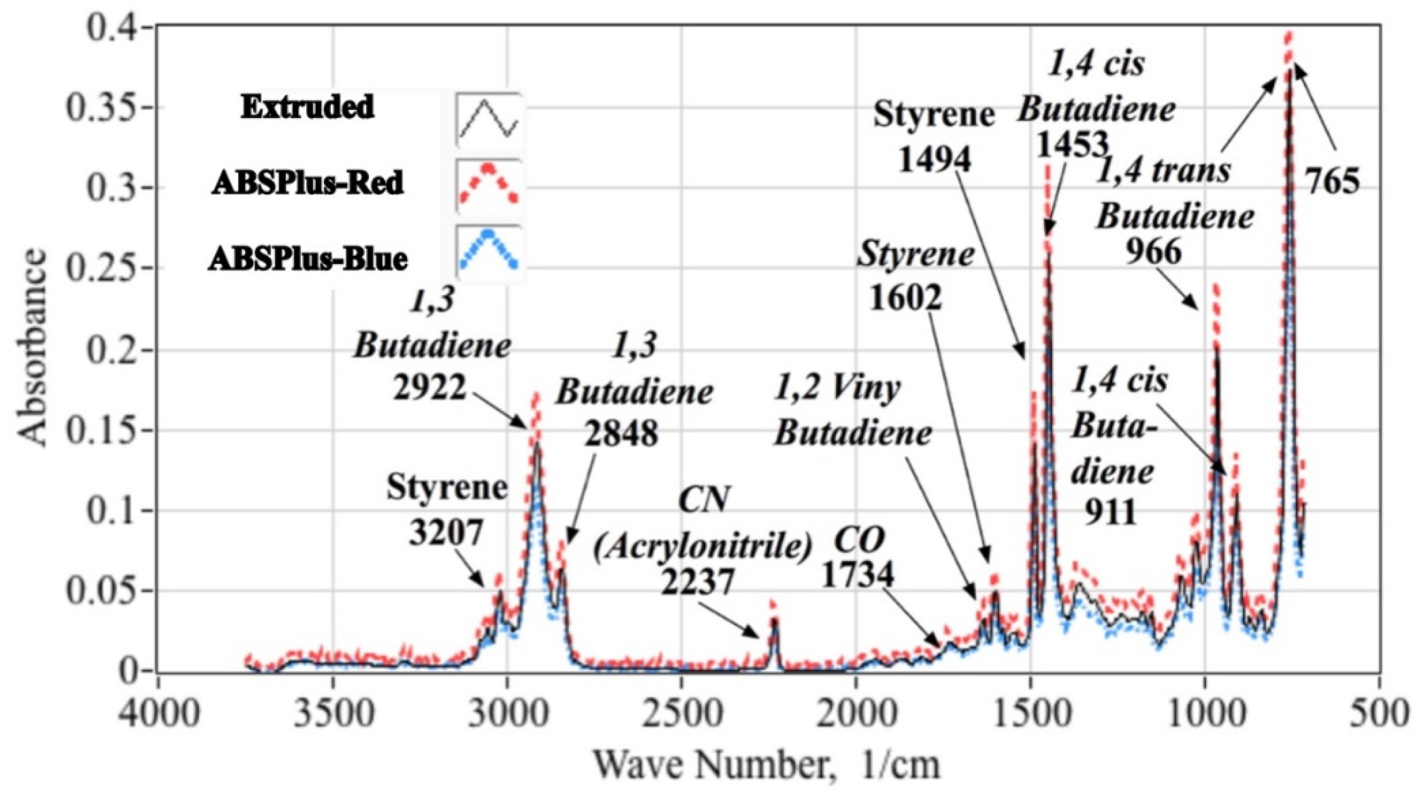
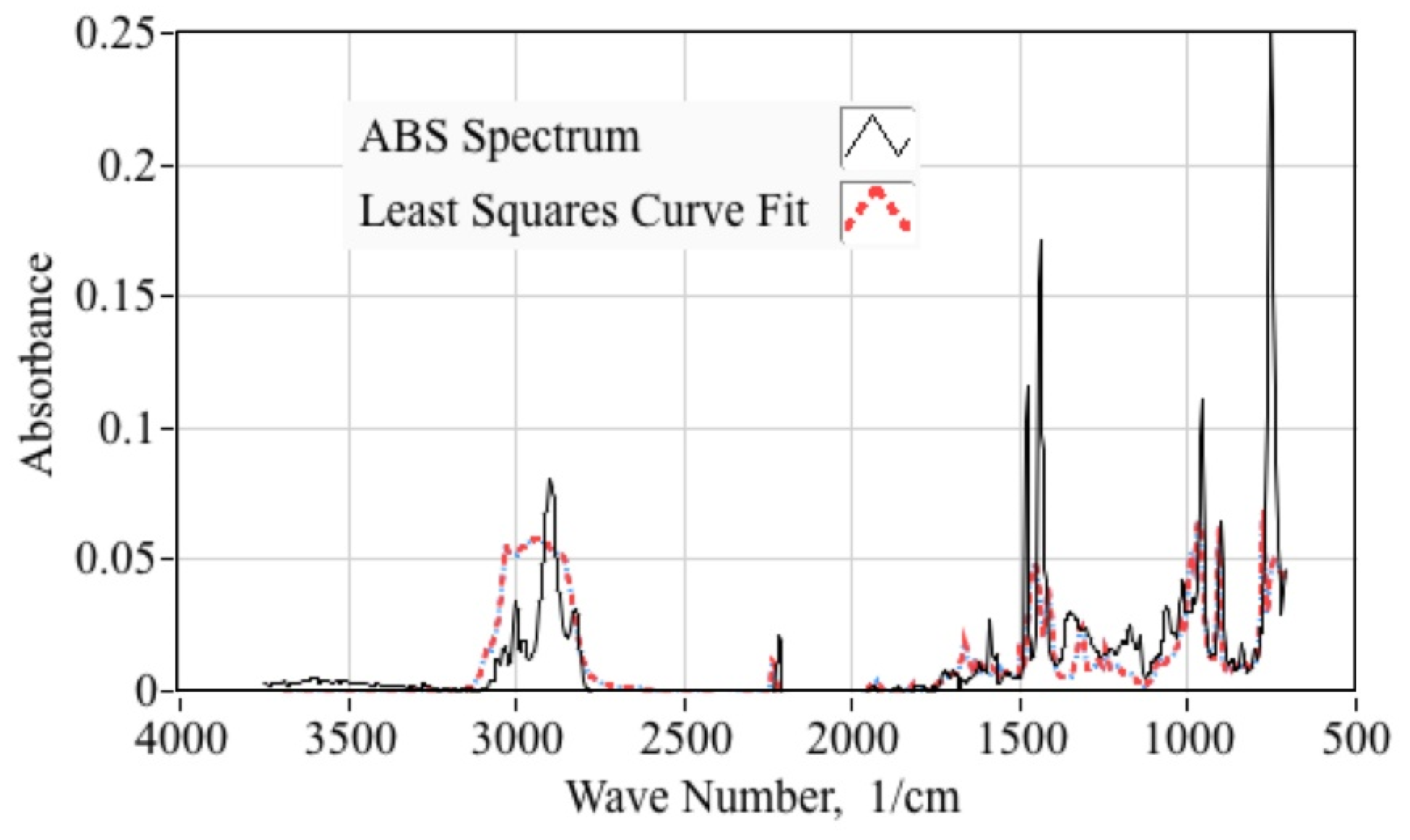
3.1. FTIR Analysis of the ABS Fuel Material

The ABS fuel used for these tests is a terpolymer material, where the constituent monomers are: (1) acrylonitrile [8], (2) butadiene [9], and (3) styrene [10]. The monomer mass fractions can vary widely for ABS preparations [11]; however, the precise chemical formulas of the various commercially available products including FDM feedstocks are tightly-held corporate secrets, and are not generally available in the public domain. Thus, in order to perform thermochemical analysis of the combustion plume, the general chemical makeups including monomer mass and mole fractions, molecular weights, and enthalpies of formation and polymerization must first be measured or estimated. This section shows the results of the chemical analysis and calculations required to estimate these properties.
Fourier transform infrared (FTIR) spectroscopy tests were performed to estimate the relative monomer proportions of both the 3-D printed (Stratasys ABSPlus-340) and extruded (McMaster-Carr, Elmhurst, IL, USA) ABS fuel materials. The specific technique used for the FTIR evaluation is known as attenuated total reflection (ATR) [12]. An ATR accessory operates by measuring changes that occur in an internally reflected infrared (IR) beam as it comes into contact with a sample. A sample is placed on a high-reflectance crystal surface, a constant pressure is applied, and the infrared signature collected from the side of the sample in contact with the crystal. An IR beam is directed onto an optically dense crystal where internal reflectance creates a rapidly attenuating (evanescent) wave that penetrates into the sample held in contact with the crystal. In regions of the IR spectrum where the sample absorbs energy, the evanescent wave will be attenuated. The attenuated beam exits the opposite end of the crystal and is directed to the detector in the IR spectrometer. The detector records the attenuated IR beam as an interferogram signal, which is subsequently used to generate the IR Fourier spectrum. Since the infrared penetration is equivalent to only a few microns, ATR is largely independent of sample thickness.
Spectra collected by this method are sensitive to the amount of pressure applied, with increasing pressure translating into primarily greater peak heights. The pressure device being used for this test series has a locking mechanism that ensures a constant pressure and allows quantitative comparison between samples. Each sample was prepared for ATR analysis by excising a small, thin area from the material surface. Once removed, the sample was placed, unexposed surface side down, on the ATR crystal surface for spectral analysis. For this test series the ATR accessory was purged with nitrogen gas and 64 scans per sample were performed with at a wavenumber resolution of 4/cm. A total of eight records were obtained for each test sample, and the associated spectra were ensemble averaged to give a measure of noise rejection.
Figure 6 compares the mean FTIR absorbance spectra obtained for two Stratasys ABS-plus (red, blue) and one extruded ABS (beige) samples. The x-axis plots the spectrum wave number in units of 1/cm, and the y-axis plots the absorbance level in fraction of absorbed power. The identifications and corresponding wavenumbers [13] of major peaks are annotated. Note that there is a high degree of similarity between the three spectra. When correlation coefficients are calculated comparing the spectra from the three different materials, the magnitudes all lie above 93%. This high level of correlation indicates practically negligible differences between the chemical compositions of the three ABS source materials used for these tests.
In order to estimate the mass proportions of each monomer in the feedstock material, the ensemble spectrum from Figure 6 was curve fit to reference spectra for acrylonitrile [14], butadiene [15], and styrene [16] assuming a linear model of the form:
A A B S ( n ) = a   A A c r y l o n i t r i l e ( n ) + b   A B u t a d i e n e ( n ) + c   A S t y r e n e ( n ) ,
with the respective absorbances of acrylonitrile, butadiene, and styrene monomers as independent variables, and the ensemble spectrum of Figure 6 as the dependent variable. The best fit coefficients {a,b,c} are evaluated for each wavenumber to give the overall minimum squared-error between the measured ABS spectrum, and the model of Equation (1). Figure 7 compares least-squares curve fit model against the ensemble spectrum for the Red ABSPlus feedstock. The resulting fit exhibits a correlations coefficient of approximately 0.85, and is deemed to be statistically significant.
The resulting mass proportions for the best-fit model of Figure 6 are: (1) acrylonitrile 28.4%, butadiene 41.4%, and styrene 30.5%. Based on the estimated mass percentages, and the associated molecular weights of the 3 ABS monomers, the corresponding mole-fractions are: (1) acrylonitrile 33.7%, (2) butadiene 47.9%, and (3) styrene 18.4%. The corresponding chemical formula is C4.399 H5.357 N0.337. Table 1 also lists the enthalpy contributions for each of the ABS copolymers including the monomer enthalpy of formation ΔHf and energy required for depolymerizing a particular monomer from the polymer chain ΔQp. Table 1 also lists the ABS material chemical formula and molecular weight Mw. The total enthalpy of the polymer is less than the sum of the enthalpies of the individual monomers and the net enthalpy contribution of each monomer given by the difference between ΔHf and ΔQp. Because the polymer reaction is exothermic, ΔQp must be returned to the fuel material in order to break the polymer bonds, and that energy is not available to support the combustion reaction.

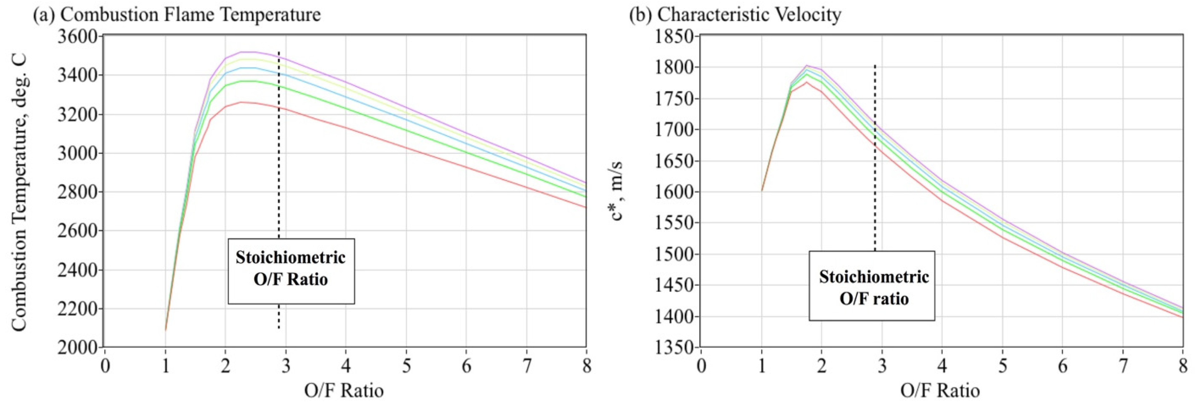
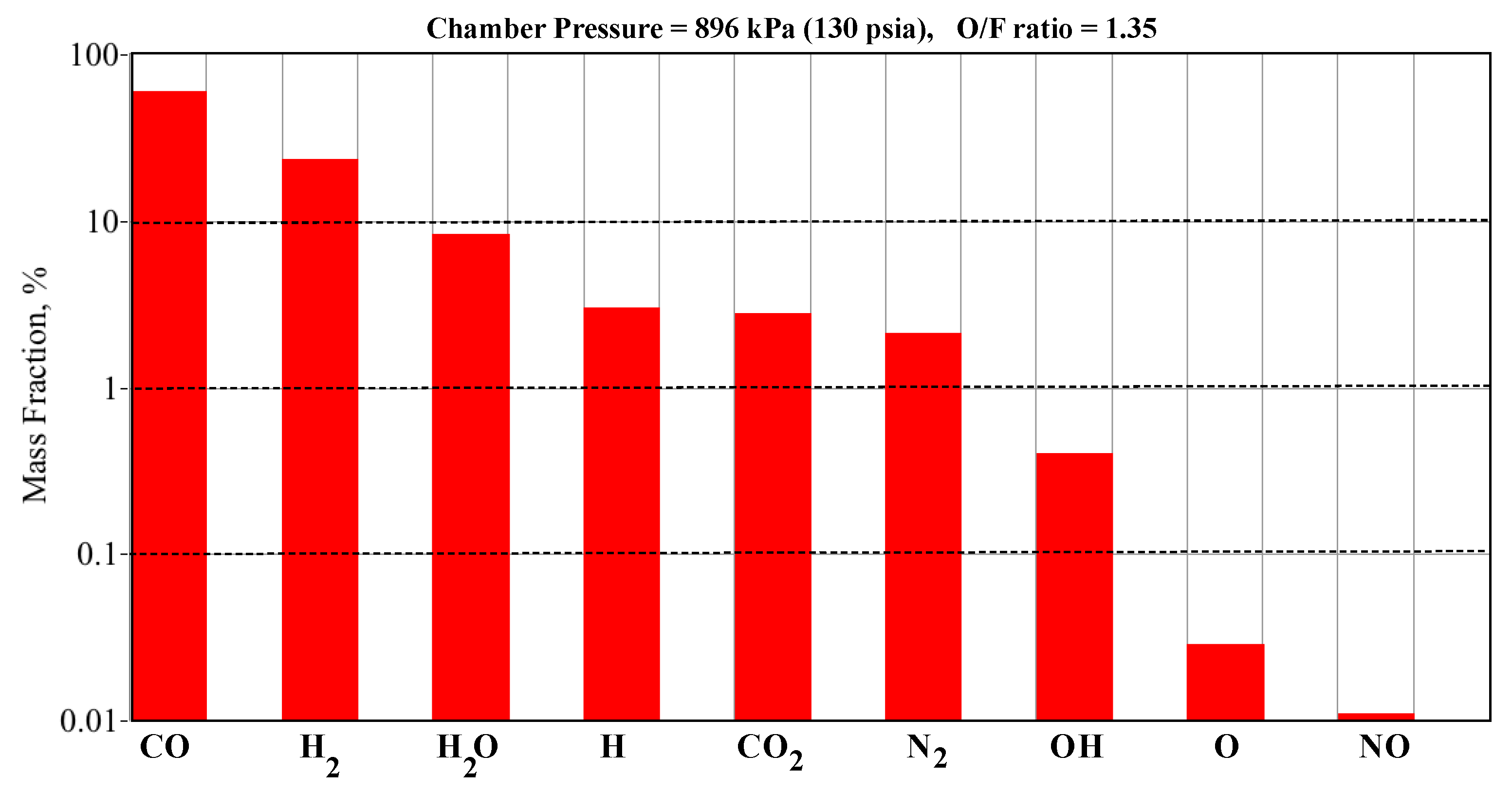
3.2. Thermochemical Analysis of the Exhaust Plume

The resulting enthalpy and molecular weight estimates from Table 1 were used to calculate the theoretical equilibrium combustion properties of ABS and gaseous oxygen as a function of the oxidizer to fuel proportions. The thermo-chemical calculations were performed using the industry-standard NASA Chemical Equilibrium with Applications (CEA) tool [22]. These calculations assume the 3-D printed fuel is burned at 100% efficiency with gaseous oxygen at various oxidizer-to-fuel (O/F) ratios. The assumed combustion (chamber) pressure P0 is allowed to vary across a range of useful combustion pressures for the GOX/ABS propellants. Figure 8 plots the theoretical flame-temperature T0 and characteristic velocity c* as a function of oxidizer-to-fuel ratio O/F. The different curves of Figure 8 represent the combustion chamber pressure levels, varying from approximately 1000 kPa (145 psia) 6000 kPa (870 psia) in 1000 kPa (145 psi) increments. Increasing values for T0 and c* are associated with the higher combustion pressures. The CEA analysis predicts the stoichiometric O/F ratio to be approximately 2.89. This value is also plotted in Figure 8a,b as the vertical dashed lines.
The CEA code also calculates the plume species concentrations for the various O/F ratios. Figure 9 shows an example bar graph that compares the species concentrations at an O/F ratio of 1.35 and a chamber pressure of 896 kPa (130 psia). Note that the predominant species are carbon monoxide, molecular hydrogen, and water vapor, with trace amounts of atomic hydrogen, carbon dioxide, molecular nitrogen, hydroxyl, and atomic oxygen. Table 2 shows the predominant emission wavelengths associated with each of these species. As shown by Table 2, the emission wavelengths of the dominant species, carbon monoxide, lie well outside of the detection range of the Hamamatsu spectrometers (640 to 1050 nm). However, for hydrogen, water vapor, and nitrogen there are emission wavelengths that lie well within the sensitivity of the spectrometers. These species, especially hydrogen and water vapor, should be identifiable in the collected emission spectra.

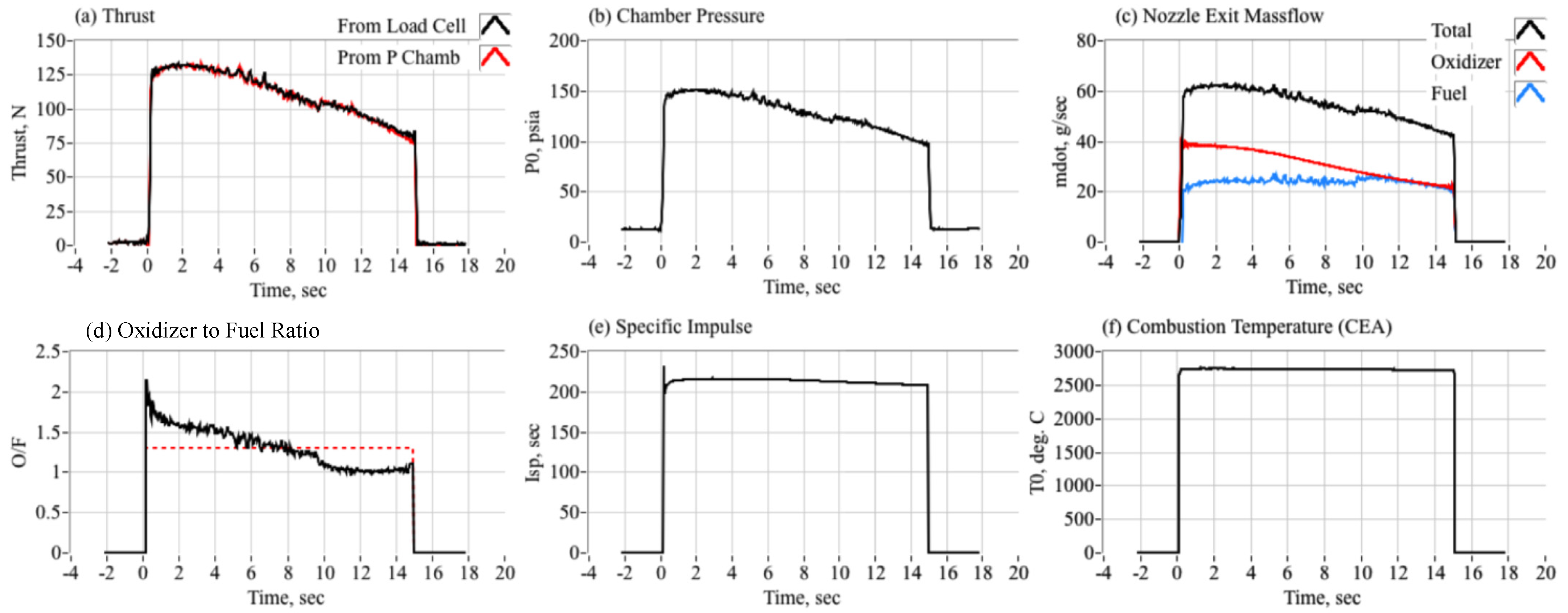
3.3. Motor Performance Analysis

This section presents the analytical methods used to calculate key performance parameters from the raw test data. These calculations include: (1) fuel mass flow rate, (2) oxidizer-to-fuel ratio, (3) equivalence ratio, (4) specific impulse, Isp, and (5) characteristic velocity. As shown by Figure 5 an inline Venturi flow meter directly measures the oxidizer flow rate in real-time; however, the test stand was not configured to directly measure the fuel mass flow. Instead, before and after each hot-firing the fuel grains were weighed to give the total fuel mass consumed during the test. These mass measurements were used to anchor the “instantaneous” fuel mass flow rates, calculated as the difference between the nozzle exit and oxidizer mass flows:
m ˙ f u e l ( t ) = m ˙ t o t a l ( t ) m ˙ o x ( t )
Knowing the nozzle throat-area A* and the plume exhaust gas properties (from the CEA analysis), the total nozzle exit mass flow was calculated from the measured chamber pressure time history P0, using the 1-dimensional choking mass flow equation, (Anderson [23], Chapter 4)
m ˙ t o t a l ( t ) = A * P 0 ( t ) γ R g T 0 ( 2 γ + 1 ) γ + 1 γ 1
The calculation of Equation (3) assumes the flow composition is frozen at the nozzle entrance, (Anderson, [23], pp. 659–661) and no nozzle erosion during the burn. For each data point in the burn time history, the two-dimensional tables of thermodynamic and transport properties from the CEA analysis were interpolated using chamber pressure P0 and mean O/F ratio as lookup variables. Calculated parameters included the gas constant Rg, ratio of specific heats γ, and flame-temperature T0. Defining the combustion efficiency as:
η * = c a c t u a l * c i d e a l * = ( γ + 1 2 γ ) γ + 1 ( γ 1 ) R g T 0 a c t u a l ( γ + 1 2 γ ) γ + 1 ( γ 1 ) R g T 0 i d e a l T 0 a c t u a l T 0 i d e a l
The theoretical flame-temperature is scaled by adjusting the combustion efficiency,
T 0 a c t u a l = η * 2 T 0 i d e a l
The calculations of Equations (2)–(5) are iterated, adjusting η* after each iteration, until the consumed fuel mass, calculated as the integral of Equation (2) over the burn duration, matches the burned fuel mass, calculated from the pre- and post-test fuel weight measurements. For this analysis the prescribed level of accuracy was 1%. Adjusting the combustion efficiency upwards has the effect of increasing the calculated fuel mass consumption, and adjusting efficiency downwards decreases the calculated fuel mass consumption. The instantaneous O/F ratio is calculated as the measured oxidizer mass flow divided by the fuel mass flow as calculated by Equation (2). Whitmore [24] derives the variational techniques used to optimize the calculation. Reference [24] also allows for nozzle erosion; however, for this test series, due to the fuel-rich motor operation, the nozzle erosion was essentially negligible.
Once the total mass flow was calculated, specific impulse and characteristic velocity were calculated using the measured thrust and chamber pressure time histories:
I s p = F t h r u s t g 0 m ˙ t o t a l   and   c * = P 0 A * m ˙ t o t a l
The thrust motor thrust was sensed directly by the test stand load cell. Thrust can also be calculated using the 1-dimensional de Laval flow equation (Anderson [23], Chapter 4), where:
F t h r u s t = P 0 A * ( 2 γ 1 ( 2 γ + 1 ) γ + 1 γ 1 ( 1 p e x i t P 0 ) γ 1 γ + ( A e x i t A * ) ( p e x i t p P 0 ) )
In Equation (7) pexit is the nozzle exit pressure calculated from the nozzle expansion ratio and chamber pressure, and p is the operating ambient pressure. A close and consistent comparison between the load-sensed and calculated thrust levels will be used to verify the verisimilitude of the previously outlined mass flow and O/F ratio calculation procedure.

4. Summary of Test Results

The section presents the test results. To date a total of five successful hot fires with burn durations varying from 5 to 25 s have been performed. Although temporary saturation of the sensors was experienced at the burn initiation, the fiber optic sensors survived for all of the hot fire tests, and both rocket performance and in-situ optical data were successfully collected for each of the five tests. The motor performance results will be presented first, followed by the spectral measurements. Motor performance data will be correlated with the optical plume measurements. Finally, the resulting optical measurements will be compared against the theoretical calculations for combustion temperature and exhaust plume species.

4.1. Motor Performance Data

Figure 10 shows representative rocket performance data collected from a 15-s burn. Plotted are thrust (Figure 10a), chamber pressure (Figure 10b), nozzle-exit mass flow (Figure 10c), oxidizer-to-fuel ratio (Figure 10d), specific impulse (Figure 10e) and the mean combustion temperature (Figure 10f). In analyzing the motor performance data, the plume exhaust thermodynamic and transport properties were provided by the earlier-described CEA analysis. As described by the previous section, the theoretical flame-temperature is scaled to estimate the “true” estimated temperature by adjusting the combustion efficiency such that the calculated fuel mass consumption matches the measured value as calculated from differences of the pre- and post-test weight measurements. Figure 11a also compares the two different thrust estimates; thrust as measured by the thrust-stand load cell and thrust as calculated from chamber pressure using the Equation (7). Figure 11c compares the nozzle exit total mass flow against the measured oxidizer mass flow and the fuel mass flow calculated by the 1-D analysis as described previously in Section 3.3. The drop off in chamber pressure and thrust results from the oxidizer tank bleed-off, where adiabatic cooling causes a large drop in the internal tank pressure. Using an oxidizer tank with a limited supply volume was instituted as a safety measure for these hot-fire tests.
Table 3 summarizes the motor performance data for the 5 burn tests. For this test series the run-to-run variability was quite small. The load-measured thrust level differs from the thrust calculated using Equation (8) by only 1.1%. This difference is within the thrust measurement margin of error, approximately 2.4%. Thus, the close comparisons between the load-sensed thrust, and the chamber pressure-based thrust calculation supports the accuracy of the fuel mass flow and O/F ratio process as described by Equations (2)–(5). Also of significance is the tO/F uncertainty of only 1.3%, with an associated flame-temperature uncertainty of approximately 50 °C. Note that the ensemble mean O/F ratio is 1.358. When compared with the stoichiometric O/F ratio of 2.89, it is clear that the test motor was operated significantly rich with an equivalence ratio, defined as the ratio of the stoichiometric O/F to the actual O/F, of approximately 2.13. The fuel rich operation results from the extended fuel grain length that was required in order to insert and separate the fiber optic cables. This fuel rich operation, coupled with the noted combustion inefficiencies, resulted in flame-temperatures and specific impulse values that are lower than have been previously achieved for GOX/ABS combustion. (Whitmore [25]) The fuel rich operation also limited any effects due to nozzle erosion during the burn.

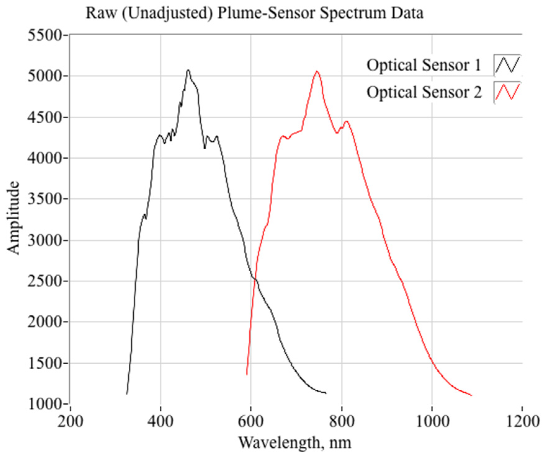
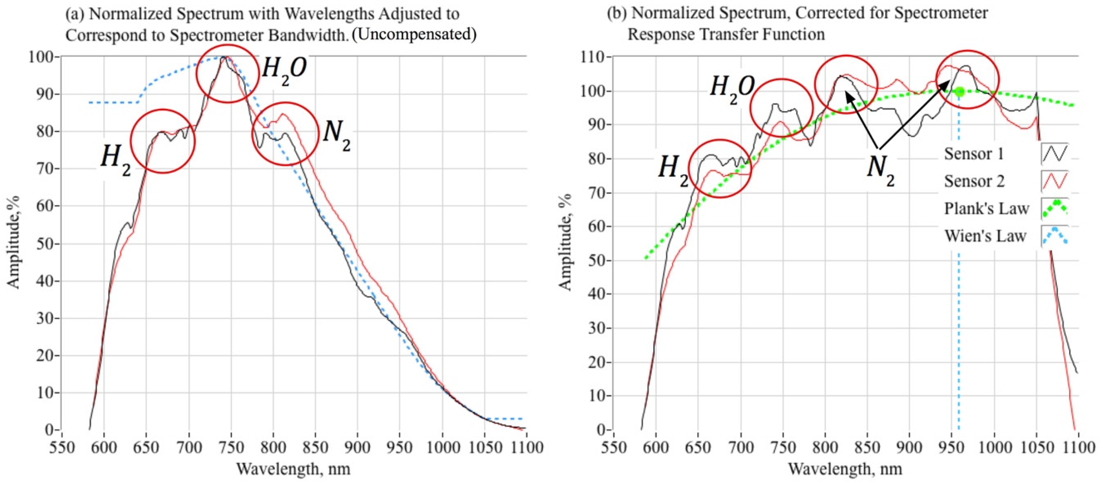
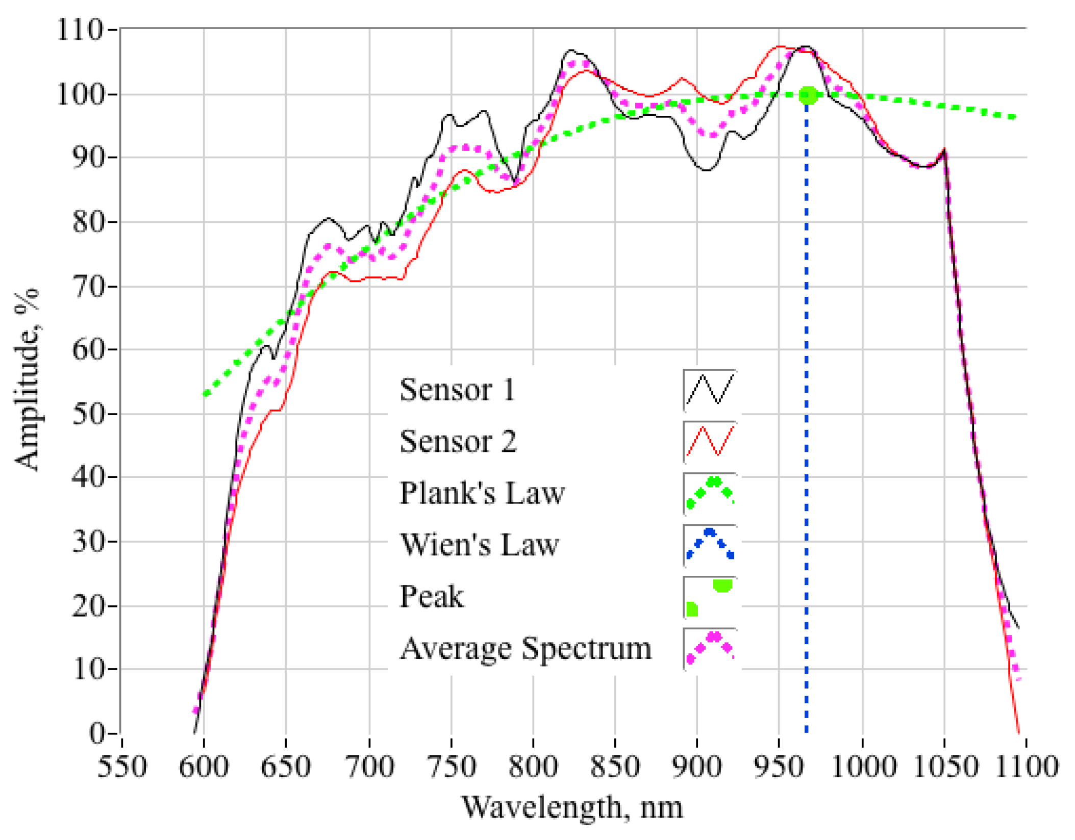
4.2. Plume Spectra Measurments

Figure 11 plots the smoothed, but unscaled spectral radiance as output by the two optical sensors, corresponding to the test data of Figure 11. These data are typical of all of the data collected during the initial testing campaign, and both the fore- and aft fiber optic locations (from Fog. 4) result in similar signatures. The plotted spectrometer data result from a 2-s ensemble average taken near the middle of the burn, approximately 6 s after ignition.
The response range from 640 to 1050 nm and transfer function (Figure 3b) of the spectrometer, are used to scale the output wavelengths and magnitudes of the raw optical sensor data. The compensation method uses the optimal deconvolution algorithm as originally developed by Norbert Wiener in the frequency domain [26]. The original method is modified to replace frequency with wavelength as the independent variable. The deconvolution algorithm amplifies attenuated spectrum wavelengths, while selectively rejecting sensor noise. The model inversion equation, as developed by Wiener, is presented by Equation (8):
S ^ ( λ ) = { ϒ ( λ ) ( S / N λ ) 2 ϒ ( λ ) 2 ( S / N λ ) 2 + 1 } S ( λ )
In Equation (8) the parameters are:
S ^ ( λ ) = adjusted   spectrum ,   calculated   as   a   function   of   the   input   wavelength ,   λ   S ( λ ) = raw   input   radiance   at   each   λ ϒ ( λ ) = spectrometer   transfer   function   coefficient   corresponding   to   λ S / N λ = signal - to - noise   ratio   at   a   given   λ
The Wiener solution weighs the spectrum coefficients to compensate for the S/N of the system as a function of the input signal wavelength. Adaptive Wiener filtering algorithms [27] that estimate the S/N as a part of the filtering process have been developed, but will not be applied here. The filter noise scaling parameter S/Nλ, although technically representing the mean-square signal-to-noise ratio of the unknown true input signal, can be approximated by the square of the signal-to-noise ratio (S/N) of the measured output signal. The S/N values were selected a priori based on the observed noise threshold of the raw spectra signals. Figure 12 shows how this S/N scaling parameter was estimated. Figure 12a plots a typical snapshot of the unfiltered-spectrum, overlaid with the spectrometer transfer function. The measured spectrum, heavily filtered with a 100-pont averaging window is also plotted. The S/N ratio is estimated by dividing the Hamamatsu transfer function coefficients, by the absolute differences between the raw and filtered spectra:
S / N λ ϒ ( λ ) | S ( λ ) n 50 n + 50 S ( λ n ) |
Figure 12b plots the estimated S/N ratio as a function of the input wavelength. This data was used for S/Nλ for all follow-on calculations.
When the spectral data of Figure 11 are compensated using the spectrometer transfer function, the result is as plotted by Figure 13. First, Figure 13a overlays the normalized and smoothed, but uncompensated, radiance data with the spectrometer transfer function. Clearly, the preponderance of the signal roll-off as a function of wavelength results from spectrometer transfer functions. Figure 13b plots the compensated spectra using the method of Equation (8), as well as the average of the two compensated spectra. The compensated spectra, measured at two different locations along the fuel port, generally agree with regard to shape and local maxima. There exist distinct “humps” at wavelengths near 656 nm, 740 nm, and 820 nm. As noted, these wavelengths correspond to H2, H2O, and N2; all species predicted in observable concentrations in the exhaust plume. The magnitude-adjusted spectral also tend to show another weak “hump” at around 950–970 nm, corresponding to second emission wavelength for N2.

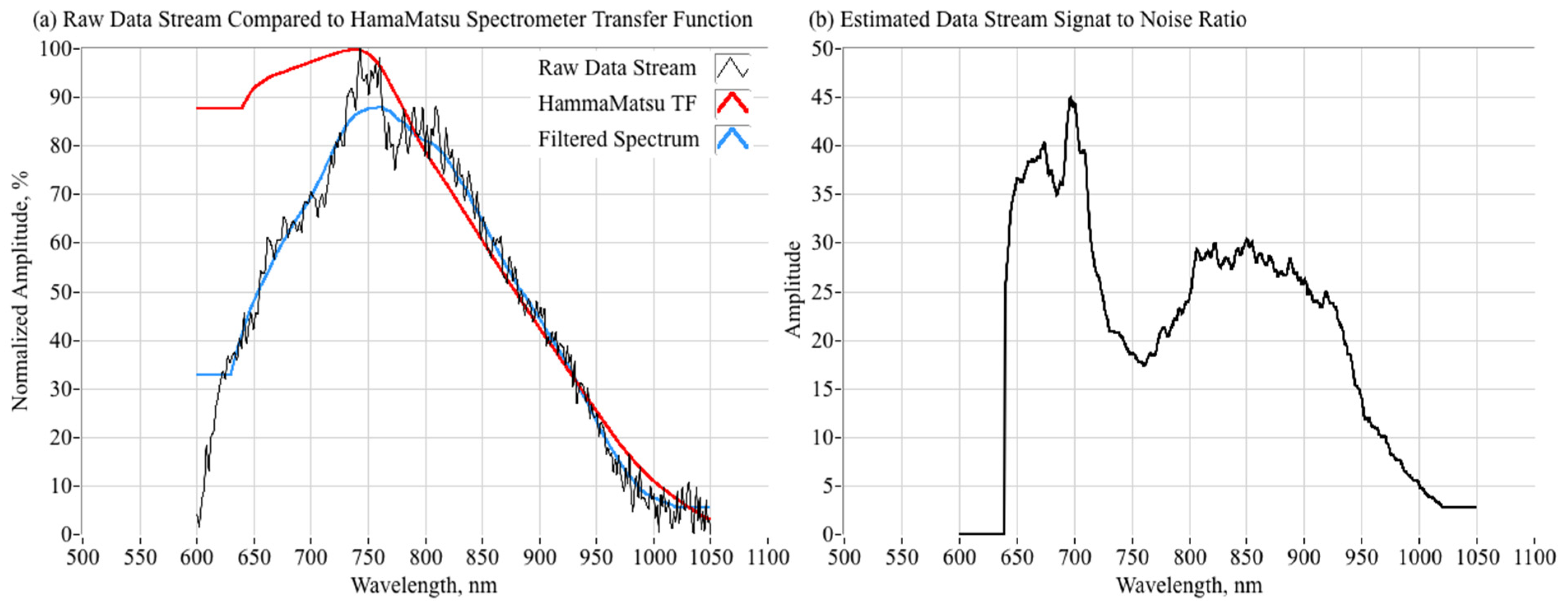
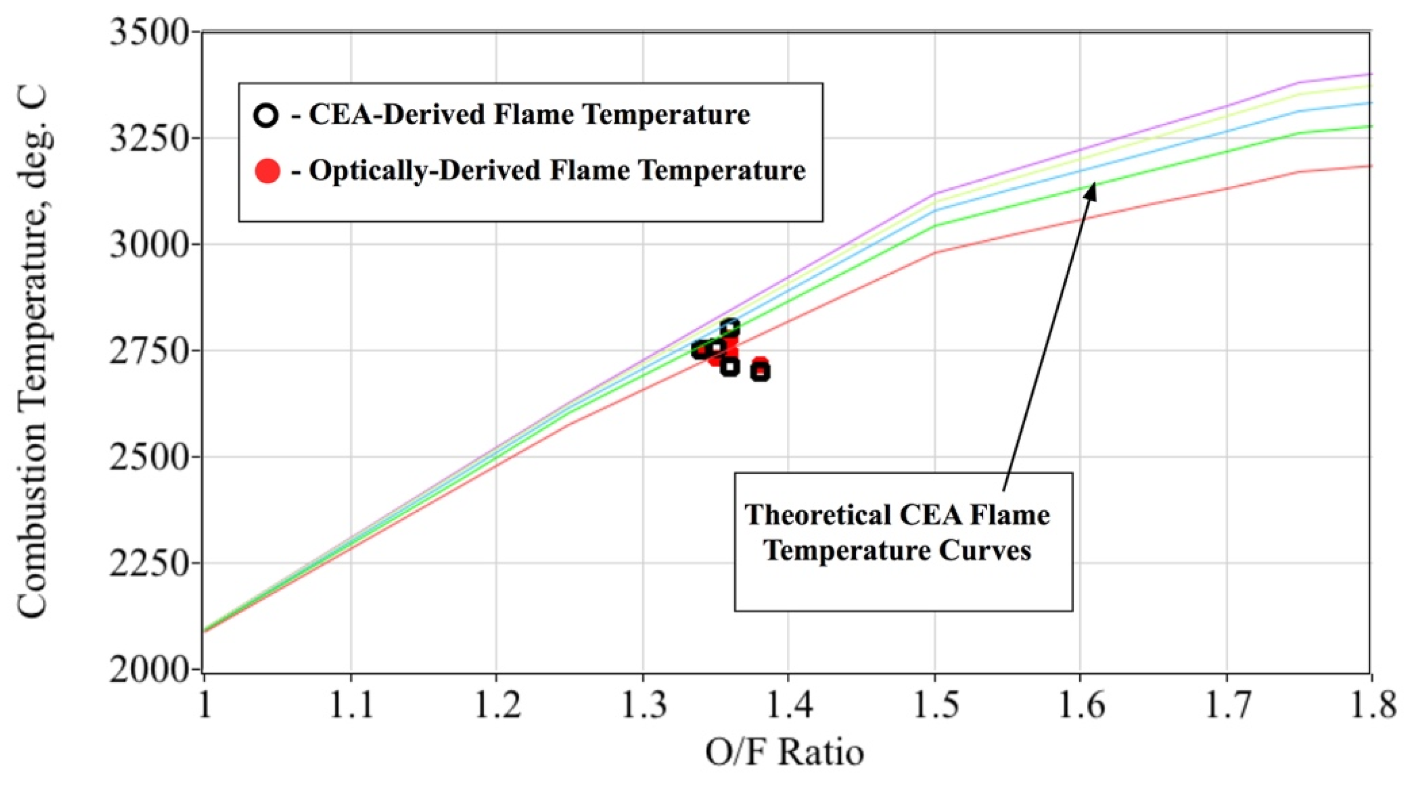
4.3. Estimating the Internal Flame-Temperature

The compensated data of Figure 13 are used to estimate the internal flame-temperature by fitting the black-body spectrum, as predicted by Planck’s Law [28]:
B A ( λ , T ) = 2 A h c 2 λ 5 1 e ( h c λ k B T ) 1
to the average of the two spectra. In Equation (10) h is Planck’s constant, c is the speed of light in a vacuum, kB is Boltzmann’s constant, lambda is the emission wavelength, T is the absolute gas temperature, and A is the amplitude scaling factor. The parameters {A,T} are the minimum-variance curve fit variables. The non-linear regression algorithm, as applied to this problem, is derived in the Appendix A of this paper. Figure 14 shows this comparison. Plotted are the data of Figure 13b overlaid with the black-body spectrum curve fit (dashed green line), and the wavelength (dashed blue line) corresponding to the curve fit maximum radiance value, approximately 957 nm. From Wien’s displacement law [29]:
T = 2.8978 × 10 3 n m K λ m a x
The corresponding gas temperature is calculated to be approximately 2755 °C. For the range of test conditions achieved during this initial testing campaign, the optically-sensed (curve-fit) flame-temperature was found to vary between 2720 °C and 2780 °C, with an ensemble mean of 2747 °C and a standard deviation of 22.5 °C. Figure 15 compares the optically-sensed flame-temperatures against those values calculated using the procedure of Equations (2)–(5) and tabulated by Table 3. The plotted O/F range has been reduced to show greater detail in the region of interest for the test motor; that is, O/F ratios between 1.0 and 2.0. The open black symbols show the CEA-derived flame-temperatures, while the closed red symbols show the optically-derived flame-temperatures for the five test burns. For reference the theoretical CEA flame-temperature curves for chamber pressures varying from 1000 to 6000 kPa are also plotted on this figure.

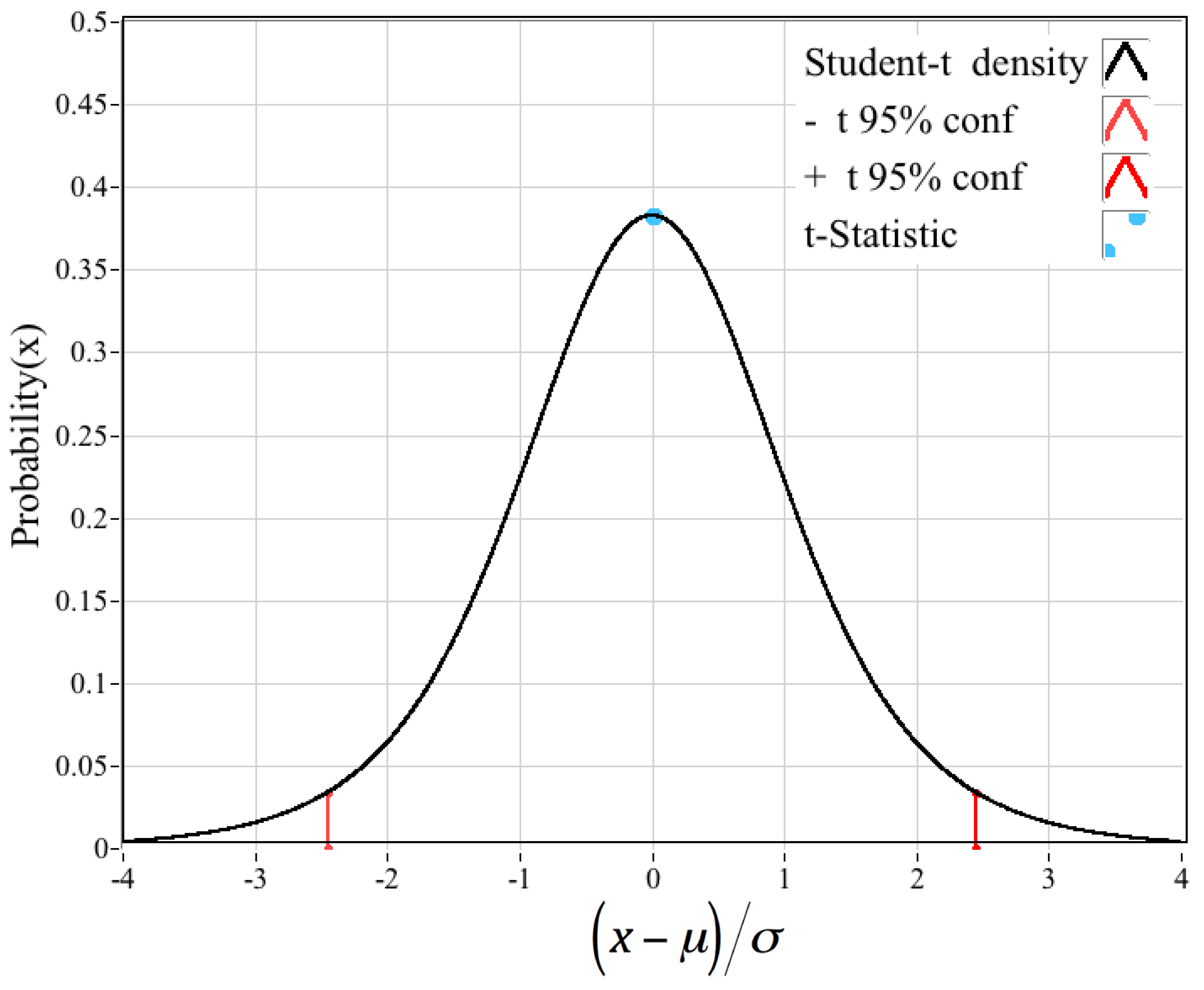
4.4. Student-t Significance Test

With such a small sample set, having only four degrees of freedom, a Student-t significance “t-test” [30] was performed to establish whether the observed differences in the two flame-temperature categories were statistically significant. The associated t-statistic for the two categories of flame-temperatures measurements, calculated as:
t s t u d e n t = | μ C E A μ o p t i c a l | 1 N ( σ C E A 2 σ o p t i c a l 2 )
is only tstudent = 0.00285. In Equation (12) N is the degrees of freedom, and {μ,σ} represent the sample mean and standard deviations for the CEA- and optically-derived flame-temperatures. Figure 16 overlays this t-statistic value on the student-t probability density curve for four degrees of freedom. The observed differences are statistically insignificant. Clearly, the limited data collected thus far demonstrate that the optically-sensed flame-temperature agrees with a very high level of confidence with the theoretically-predicted values.

5. Proposed Future Work

The in-situ data set resulting from this initial testing campaign is very promising, but far from definitive. Although qualitatively successful in demonstrating the feasibility of the optical sensing method, the early experiments mostly achieved quantitative results for a very limited data range. The Hamamatsu spectrometer calibrations used for this analysis rely only on the manufacturer’s specifications for the optical transfer function and the detection frequency range; thus, the absolute accuracy of the sensed optical radiance and the associated wavelengths is unclear. Also, because the spectrometer range was limited to the low visible and high-infrared wavelengths, the dominant species-CO-was not identifiable.
Proposed follow-on activities will not only develop a more capable optical sensor package but will broaden the associated analytical methods to produce verifiably accurate quantitative results. The enhanced optical system will extend the measurement spectrum from approximately 300 nm (ultraviolet spectrum) to 1200 nm (mid-IR) in order to detect exhaust species not identifiable with the original prototype system. The wavelength calibration of the upgraded system will be assessed by blending the printed feedstock with additives such as copper, iron, graphite, or aluminum with known spectral emission wavelengths. In this approach the known spectral lines of the additive materials would provide very precise wavelength benchmarks. Using these infused feed stock grain will allow the calibration to be substantially improved. Previously, ABS feed stock has been infused with copper powders with relative weights of 2, 4, and 6% [31], so this is a well-established methodology.
Although the in-situ sensor was demonstrated to successfully survive for up to 25 s of burn time, the initial testing campaign did not attempt to characterize the fiber optic cable durability, and its ability to survive multiple burn cycles. For the preliminary testing campaign, the embedded cables were replaced after each burn. Similarly, the survivability of the embedded fiber-optic cables under high vibration environments was not addresses. Follow-on testing activities will also seek to determine the survivability of the bedded cables for multiple burn cycles, and under high dynamic vibration loads.
Because of the limited O/F ratios achieved during the preliminary testing campaign, the flame temperature did not vary substantially, by only 100 °C over the entire test ensemble. Securing test data over a wider range of test conditions is clearly desirable. Proposed follow-on efforts will operate the system at a higher chamber pressures and will retrofit the 75-mm test systems with a v-slot ball valve to allow a wide throttling range, from approximately 100% to less than 20%. These modifications will allow a significantly wider range of O/F ratios to be achieved, providing a wider range of flame temperatures and exhaust species concentrations. These test-system changes will significantly challenge the optical measurement systems and will allow a more comprehensive statistical assessment of the overall system accuracy.

6. Conclusions

Preliminary results from this testing campaign demonstrate the presented in-situ optical sensing technique as offering considerable promise. Based on this preliminary analysis, it appears that significant quantitative information can be extracted from the in-situ measurements. The presented method provides the capability for minimally intrusive sensing of the combustion flame temperature, and potentially allows direct measurements of species concentrations. To date a total of five successful hot fires with burn durations varying from 5 to 25 s have been performed. The fiber optic sensors survived for all of the hot fire tests, and both rocket performance and in-situ optical data were successfully collected for each of the five tests. Test results demonstrate that the receding fiber optic tip still transmits light through the cable. The local radiance maxima in the optical spectra curves correspond closely with known the emission frequencies of atomic and molecular hydrogen, water vapor, and molecular nitrogen; all species that are predicted by the theoretical analysis to exist in the combustion plume.
Applying Planck and Wien’s law to the sensitivity-adjusted spectra calculate a radiant gas temperature that closely agrees with theoretical calculations. Using Wien’s displacement law, the corresponding ensemble gas temperatures are calculated to range between approximately 2720 °C and 2780 °C, with an ensemble mean of 2747 °C and a standard deviation of 22.5 °C. When a Student-t significance test is performed on the two flame-temperature categories, the associated only t-statistic shows that the observed temperature differences are statistically insignificant. Thus, it is concluded that the optically-sensed flame-temperature agrees with a very high level of confidence with the theoretically-predicted values. Clearly, the simple in-situ measurement system operates as designed, and it shows considerable promise for future applications to a wide swath of gas-generator systems.

Author Contributions

Conceptualization, S.J.P.; methodology, S.J.P. and S.A.W.; software, S.A.W. and C.I.F.; validation, S.A.W. and C.I.F.; formal analysis, S.A.W.; investigation, S.A.W. and C.I.F.; resources, S.A.W. and S.J.P.; data curation, S.A.W.; writing, original draft preparation, S.A.W.; writing, revision and editing, S.A.W., S.J.P. and C.I.F.; visualization, S.A.W.; supervision, S.A.W.; project administration, S.A.W.; funding acquisition, S.A.W. and S.J.P. All authors have read and agreed to the published version of the manuscript.

Funding

This work was partially funded with a cooperative agreement between Weber State University, Utah State University, and Northrop Grumman Corporation. Funds were also provided by the Utah NASA Space Grant Consortium.

Institutional Review Board Statement

None required.

Informed Consent Statement

None required.

Data Availability Statement

Data available on request due to potential proprietary restrictions.

Acknowledgments

The authors are especially grateful for the assistance of Dixon Nielson, Utah State College of Engineering Business Manager for coordinating with, and securing funding for, the senior design teams supporting this project.

Conflicts of Interest

The authors declare no conflict of interest.

Nomenclature

Symbols
A Average absorbance of total polymer
{a,b,c}FTIR least-squares curve fit coefficients
Aamplitude scaling factor
Acfuel port cross-sectional area, cm2
Aexitnozzle exit area, cm2
A*sectional area at which local flow chokes, cm2
A residual vector for estimated amplitude
Bblack body spectral radiance, W/rad2-m3
cspeed of light in a vacuum, 2.998 × 10⁸ m/s
c*characteristic velocity of propellants, m/s
Fcurve fit function, W/rad2-m3
Fthrustthrust level, N
g0normal acceleration of gravity at sea level, 9.8067 m/s2
hPlanck’s constant, 6.62607015 × 10⁻³⁴ J/Hz
iwavelength index
jiteration index
kBBoltzmann constant, 1.380649 × 10⁻²³ J/K
m ˙ f u e l fuel mass flow, g/s
m ˙ o x oxidizer mass flow, g/s
m ˙ t o t a l total mass flow through the nozzle, g/s
Ndegrees of freedom
nnumber of wavelength points in a given spectrum
O/Foxidizer-to-fuel ratio
pexitnozzle exit pressure, kpa
poperating ambient pressure, kpa
P0combustion chamber pressure, kpa
Sspectrum radiance at a single data point, W/rad2-m3
S residual vector for estimated radiance, W/rad2-m3
S ^ spectrum radiance adjusted for spectrometer response transfer function, W/rad2-m3
S/Nλmeasured spectrum signal to noise ratio at a given wavelength
Tradiant temperature, K
T0stagnation temperature, K
tstudentstudent t-statistic value
tburnburn time, s
T residual vector for estimated temperature, K
Xestimation coefficient vector
ΓJacobian Matrix
ΔHf Molar enthalpy of formation, kJ/g-mol
ΔQp Molar enthalpy of polymerization, kJ/g-mol
Φequivalence ratio
λwavelength, nm
λmaxwavelength of maximum radiance, nm
ϒ spectrometer response transfer function
μmean value
σstandard deviation
η*combustion efficiency
γratio of specific heats
Acronyms
ABSAcrylonitrile Butadiene Styrene
ATRAttenuated Total Reflection
BLASTBattery and Survivability Limits Testing
CEAChemical Equilibrium with Applications
CMOSComplementary Metal Oxide Semiconductor
FDMFused Deposition Manufacturing
FTIRFourier Transform InfraRed Spectroscopy
GOXGaseous Oxygen
HVPSHigh Voltage Power Supply
IRInfraRed
P&IDPiping and Instrumentation
USUUtah State University

Appendix A. Non-Linear Regression Algorithm for Fitting Planck’s Law to the Optical Sensor Data

This section derives the non-linear least squares algorithm used to calculate the “best fit”, of Planck’s law to the ensemble average of the spectrum data sets as presented by Figure 13. The derivation of the iteration algorithm is presented first. The derivations for the functional derivatives are presented after the regression algorithm derivation.

Appendix A.1. Derivation of the Non-Linear Regression Algorithm

First, assume an arbitrary amplitude parameter “A” to give the best match to the observed spectrum amplitude. The resulting function is:
F ( A , T ) B A ( λ , T ) = 2 A h c 2 λ 5 1 e ( h c λ k B T ) 1
The observed “n” spectrum data points over the operating band of the spectrometer are:
S | 1 n = { S ( 1 ) ,   S ( 2 )   S ( n ) }
Expanding F(A,T) in a Taylor’s series for wavelength “i” corresponding to an arbitrary single data point in the spectrum, about some initial guess for the parameters (A(j),T(j)):
S ( i ) = F ( i ) ( A ( j ) , T ( j ) ) + { F A } ( i ) ( j ) ( A ( j + 1 ) A ( j ) ) + { F T } ( i ) ( j ) ( T ( j + 1 ) T ( j ) ) + h . o . t .
Truncating after first order, and writing the equivalence for each wavelength corresponding to each data point in the observed spectrum:
[ S ( 1 ) S ( 1 ) . . . S ( n 1 ) S ( n ) ] [ F ( 1 ) ( A ( j ) , T ( j ) ) F ( 2 ) ( A ( j ) , T ( j ) ) . . . F ( n 1 ) ( A ( j ) , T ( j ) ) F ( n ) ( A ( j ) , T ( j ) ) ] = [ { F A } ( 1 ) ( j ) { F T } ( 1 ) ( j ) { F A } ( 2 ) ( j ) { F T } ( 2 ) ( j ) . . . . . . { F A } ( n 1 ) ( j ) { F T } ( n 1 ) ( j ) { F A } ( n ) ( j ) { F T } ( n ) ( j ) ] [ A ( j + 1 ) A ( j ) T ( j + 1 ) T ( j ) ]
Simplify Equation (A3) by defining the substitutions:
S ( i ) S ( i ) F ( i ) ( A ( j ) , T ( j ) ) A ( j + 1 ) A ( j + 1 ) A ( j ) T ( j + 1 ) T ( j + 1 ) T ( j ) X j + 1 ) = [ A ( j + 1 ) T ( j + 1 ) ] Γ ( j ) = [ { F A } ( 1 ) ( j ) { F T } ( 1 ) ( j ) . . . . . . { F A } ( n ) ( j ) { F T } ( n ) ( j ) ]
and Equation (A4) is written in more compact for as:
S ( j + 1 ) = Γ ( j ) Χ ( j + 1 )
Solving for the minimum-variance curve fit using the pseudo-inverse method [32]:
Χ ( j + 1 ) = [ Γ ( j ) T Γ ( j ) ] 1 Γ ( j ) T S ( j + 1 )
By applying Cramer’s rule [33], Equation (A6) is written in closed form, explicitly in terms of the original variables as:
[ A ( j + 1 ) T ( j + 1 ) ] = [ A ( j ) T ( j ) ] + [ i = 1 N ( { F T } ( i ) ( j ) ) 2 i = 1 n ( { F A } ( i ) ( j ) { F T } ( i ) ( j ) ) i = 1 n ( { F A } ( i ) ( j ) { F T } ( i ) ( j ) ) i = 1 n ( { F A } ( i ) ( j ) ) 2 ] [ i = 1 n ( { F A } ( i ) ( j ) [ S ( i ) F ( i ) ( A ( j ) , T ( j ) ) ] ) i = 1 n ( { F A T } ( i ) ( j ) [ S ( i ) F ( i ) ( A ( j ) , T ( j ) ) ] ) ] i = 1 N ( { F A } ( i ) ( j ) ) 2 i = 1 N ( { F T } ( i ) ( j ) ) 2 ( i = 1 n ( { F A } ( i ) ( j ) { F T } ( i ) ( j ) ) ) 2

Appendix A.2. Derivatives of Planck’s Function

Writing the original function in terms of the “ith” wavelength:
F ( i ) ( A , T ) 2 A h c 2 λ ( i ) 5 1 e ( h c λ ( i ) k B T ) 1 ,
then the partial derivative with respect to “A” is simply:
{ F A } = 2 h c 2 λ ( i ) 5 1 e ( h c λ ( i ) k B T ) 1
Similarly, the derivative with respect to “T” is:
{ F T } = 2 A ( h 2 c 3 λ ( i ) 6 k B T 2 ) e ( h c λ ( i ) k B T ) ( e ( h c λ ( i ) k B T ) 1 ) 2
Equations (A7), (A8) and (A10) constitute the collected solution algorithm. Starting with an initial guess for the parameters (A(j),T(j)), Equation (A7) is iterated using successive substitutions until the differences between iterations for the parameters become acceptably small. The resulting solution gives the minimum variance fit between Planck’s law and the observed spectra. Only the data that lie between the sensitivity limits of the spectrometer, between 640 and 1050 nm, were allowed into the data set that were fit to Equation (A1).

References

  1. Gardon, R. An instrument for the direct measurement of intense thermal radiation. Rev. Sci. Instrum. 1954, 24, 366–370. [Google Scholar] [CrossRef]
  2. Kidd, C.T.; Nelson, C.G. How the Schmidt-Boelter gage really works. In Proceedings of the 41st 41st International Instrumentation Symposium, Research Triangle Park, NC, USA, 7–11 May 1995; pp. 347–368. [Google Scholar]
  3. HAMAMATSU MS Series Mini-Spectrometers. Available online: https://www.hamamatsu.com/resources/pdf/ssd/c10988ma-01_etc_kacc1169e.pdf (accessed on 24 December 2021).
  4. Whitmore, S.A.; Armstrong, I.W.; Heiner, M.C.; Martinez, C.J. High-performing hydrogen peroxide hybrid rocket with 3-D printed and extruded ABS fuel. Aeronaut. Aerosp. Open Access J. 2018, 2, 356–388. [Google Scholar] [CrossRef] [Green Version]
  5. Whitmore, S.A.; Martinez, C.J.; Merkley, D.P. Catalyst development for an arc-ignited hydrogen peroxide/ABS hybrid rocket system. Aeronaut. Aerosp. Open Access J. 2018, 2, 356–388. [Google Scholar] [CrossRef] [Green Version]
  6. Whitmore, S.A.; Babb, R.S.; Gardner, T.J.; LLoyd, K.P.; Stephens, J.C. Pyrolytic graphite and boron nitride as low-erosion nozzle materials for long-duration hybrid rocket testing, AIAA 2020–3740. In Proceedings of the AIAA Propulsion and Energy 2020 Forum, Virtual Event, 24–28 August 2020. [Google Scholar]
  7. Whitmore, S.A.; Inkley, N.R.; Merkley, D.P.; Judson, M.I. Development of a power-efficient, restart-capable arc ignitor for hybrid rockets. J. Propuls. Power 2015, 31, 1739–1749. [Google Scholar] [CrossRef]
  8. Anon. National Institute for Standards in Technology (NIST) Standard Reference Database Number 69. Available online: http://webbook.nist.gov/chemistry (accessed on 1 June 2019).
  9. Othmer, K. Butadiene. In Encyclopedia of Chemical Technology; John Wiley & Sons, Inc.: New York, NY, USA, 2006. [Google Scholar]
  10. Anon. Styrene. National Library of Medicine. PubChem. Available online: https://pubchem.ncbi.nlm.nih.gov/compound/Styrene (accessed on 12 August 2021).
  11. Cha, J. Acrylonitrile-Butadiene-Styrene (ABS) Resin. In Engineering Plastics Handbook; Margolis, J.M., Ed.; McGraw-Hill: New York, NY, USA, 2006; pp. 101–130. [Google Scholar]
  12. Bradley, M. FTIR Sample Techniques: Attenuated Total Reflection (ATR). Thermo Fisher Scientific Technical Note. Available online: https://www.thermofisher.com/us/en/home/industrial/spectroscopy-elemental-isotope-analysis/spectroscopy-elemental-isotope-analysis-learning-center/molecular-spectroscopy-information/ftir-information/ftir-sample-handling-techniques.html (accessed on 1 June 2019).
  13. Junga, M.R.; Horgena, F.D.; Orskib, S.V.; Rodriguez, V.C.; Beers, K.L.; Balazs, G.H.; Jones, T.T.; Work, T.M.; Brignace, K.C.; Royer, S.J.; et al. Validation of ATR FT-IR to identify polymers of plastic marine debris, including those ingested by marine organisms. Mar. Pollut. Bull. 2018, 127, 704–716. [Google Scholar] [CrossRef] [PubMed]
  14. Smith, A.L.; Carver, C.D. (Eds.) Propene Nitrile. In The Coblentz Society Desk Book of Infrared Spectra, 2nd ed.; The Coblentz Society: Kirkwood, MO, USA, 1982; pp. 1–24. Available online: https://webbook.nist.gov/cgi/cbook.cgi?JCAMP=C107131&Index=1&Type=IR (accessed on 1 June 2019).
  15. Smith, A.L.; Carver, C.D. (Eds.) Butadien. In The Coblentz Society Desk Book of Infrared Spectra, 2nd ed.; The Coblentz Society: Kirkwood, MO, USA, 1982; pp. 1–24. Available online: https://webbook.nist.gov/cgi/cbook.cgi?JCAMP=C107131&Index=1&Type=IR (accessed on 1 June 2019).
  16. Smith, A.L.; Carver, C.D. (Eds.) Styrene. In The Coblentz Society Desk Book of Infrared Spectra, 2nd ed.; The Coblentz Society: Kirkwood, MO, USA, 1982; pp. 1–24. Available online: https://webbook.nist.gov/cgi/cbook.cgi?JCAMP=C100425&Index=1&Type=IR (accessed on 1 June 2019).
  17. Baxendale, J.L.H.; Madaras, G.W. Kinetics and heats of copolymerization of acrylonitrile and methyl methacrylate. J. Polym. Sci. 1956, 19, 171–179. [Google Scholar] [CrossRef]
  18. Seymour, R.B.; Carraher, C.E., Jr. Polymer Chemistry, Revised and Expanded, 6th ed.; Marcel Dekker Publishing, Inc.: New York, NY, USA, 2003; Available online: https://www.academia.edu/29185976/Seymour_Carrahers_Polymer_Chemistry_Sixth_Edition (accessed on 5 December 2021).
  19. Van Krevelen, D.W.; Jijenhuis, K. Properties of Polymers: Their Correlation with Chemical Structure; Their Numerical Estimation and Prediction from Additive Group Contributions, 4th ed.; Elsevier Science Ltd.: Amsterdam, The Netherlands, 2009. [Google Scholar]
  20. Prosen, E.J.; Maron, F.W.; Rossini, F.D. Heats of combustion, formation, and isomerization of ten C4 hydrocarbons. J. Res. 1951, 46, 106–112. [Google Scholar]
  21. Prosen, E.J.; Rossini, F.D. Heats of formation and combustion of 1,3-butadiene and styrene. J. Res. 1945, 34, 59–63. [Google Scholar] [CrossRef]
  22. Gordon, S.; McBride, B.J. Computer Program for Calculation of Complex Chemical Equilibrium Compositions and Applications; NASA RP-1311; NASA: Washington, DC, USA, 1994. [Google Scholar]
  23. Anderson, J.D. Modern Compressible Flow, 3rd ed.; The McGraw Hill Companies, Inc.: New York, NY, USA, 2003; Chapter 4; pp. 127–187, ISBN-13 978-0072424430; Available online: https://libcat.lib.usu.edu/search/i0070016542 (accessed on 5 December 2021).
  24. Whitmore, S.A. A variational method for estimating time-resolved hybrid fuel regression rates from chamber pressure. In Proceedings of the AIAA 2020-3762, AIAA Propulsion and Energy Forum 2020, Virtual Event, 24–28 August 2020. [Google Scholar] [CrossRef]
  25. Whitmore, S.A. Nytrox as “drop-in” replacement for gaseous oxygen in SmallSat hybrid propulsion systems. Aerospace 2000, 7, 43. [Google Scholar] [CrossRef] [Green Version]
  26. Meditch, J.S. Stochastic Optimal Linear Estimation and Control; McGraw-Hill: New York, NY, USA, 1969; pp. 288–322. [Google Scholar]
  27. Gonzalez, R.; Woods, R.; Eddins, S. Digital Image Processing Using Matlab; Prentice Hall: Saddle River, NJ, USA, 2003; Chapter 4. [Google Scholar]
  28. Dougal, R.C. The Presentation of the Planck Radiation Formula (Tutorial). Phys. Educ. 1976, 11, 438–443. [Google Scholar] [CrossRef]
  29. Walker, J. Fundamentals of Physics, 8th ed.; John Wiley and Sons: Hoboken, NJ, USA, 2008; p. 891. ISBN 9780471758013. [Google Scholar]
  30. Beckwith, T.G.; Marangoni, R.D.; Lienhard, V.J.H. Mechanical Measurements, 6th ed.; Prentice Hall: Hoboken, NJ, USA, 2006; pp. 43–73. [Google Scholar]
  31. Whitmore, S.A.; Olsen, K.C.; Forster, P.; Oztan, C.; Coverstone, V.L. Test and evaluation of copper-enhanced, 3-D printed ABS hybrid rocket fuels. In Proceedings of the AIAA 2021-3225, AIAA Propulsion and Energy 2021 Forum, Virtual Event, 9–11 August 2021. [Google Scholar]
  32. Boyd, S. Lecture 5, Least-squares, EE263 Lecture Notes. 2007. Available online: https://see.stanford.edu/materials/lsoeldsee263/05-ls.pdf (accessed on 25 May 2021).
  33. Kosinski, A.A. Cramer’s Rule is due to Cramer. Math. Mag. 2001, 74, 310–312. [Google Scholar] [CrossRef]
Figure 1. Typical Gardon Gauge Installation. (Wikimedia Commons, free media repository, public domain). (a) Schmidt -Boelter Gardon Gauge (Wikimedia Commons, public domain). (b) Typical Installation. (c) Heat Flux Paths.
Aerospace 09 00057 g001
Figure 2. Proof-of-Concept Tests for Fiber-Optic Sensor. (a) Fiber Optic Fed Through EPDM Rubber Sample. (b) Burning the EPDM/Fiber Optic Sample. (c) Fiber Optic Cable with Melted Tip, Still Transmitting Light.
Aerospace 09 00057 g002
Figure 3. Hamamatsu Optical Sensing System Components. (a) Fiber Optic Connection to Spectrometer via Custom Adapter. (b) Spectrometer Transfer Function. (c) Block Diagram of the Optical Sensor Electronics and Data Acquisition.
Aerospace 09 00057 g003
Figure 4. Legacy 75 mm Hybrid Motor Adapted for Fiber-Optic Measurement Tests.
Aerospace 09 00057 g004
Figure 5. Motor Test Systems Piping and Instrumentation Diagram.
Aerospace 09 00057 g005
Figure 6. Ensemble Mean FTIR Spectra for ABS Material Samples: ABSPlus-Red, ABS Plus-Blue, and Extruded.
Aerospace 09 00057 g006
Figure 7. Least Squares Curve Fit Model Compared to Ensemble Spectrum for MakerBot ABS.
Aerospace 09 00057 g007
Figure 8. Theoretical Flame-temperature and c* for GOX/ABS Combustion.
Aerospace 09 00057 g008
Figure 9. Theoretical GOX/ABS Plume Exhaust Species for O/F Ratio 1.35 (Φ = 2.14).
Aerospace 09 00057 g009
Figure 10. Motor Performance Results from a 15-s Hot Fire Test.
Aerospace 09 00057 g010
Figure 11. Unscaled Ensemble Spectrum Corresponding to Burn Data of Figure 11.
Aerospace 09 00057 g011
Figure 12. Estimating the Spectrometer Sensor Signal-to-Noise Ratio.
Aerospace 09 00057 g012
Figure 13. Plume Optical Sensor Spectra, Adjusted for Spectrometer Response Sensitivity.
Aerospace 09 00057 g013
Figure 14. Planck’s Law Fit of Compensated Spectra Data.
Aerospace 09 00057 g014
Figure 15. Comparing CEA-Derived to Optically-Derived Flame-Temperatures.
Aerospace 09 00057 g015
Figure 16. Comparing Flame-Temperature t-Statistic with. Student-t Probability Curve for 4 Degrees of Freedom.
Aerospace 09 00057 g016
Table 1. Enthalpy of Formation Contributions of Copolymers in the MakerBot ABS Formulation.
MonomerChemical FormulaMw g/molΔHf Monomer
kJ/g-mol
ΔQp Polymer
kJ/g-mol
Net ΔHf kJ/g-molMole FractionMass FractionNet Enthalpy Contribution
kJ/g-mol
Acrylo-nitrileC3H3N53.06172.62 [17]74.3 [18]98.310.3370.28433.13
ButadieneC4H654.09104.10 [19]72.10 [20]32.000.4790.41115.33
StyreneC8H8104.15146.91 [21]84.60 [20]63.310.1840.30511.65
ABS TotalC4.399 H5.357 N0.37762.95 1.001.0060.11
Table 2. Emission Wavelength Associated with Known Plume Exhaust Species.
SpeciesMass FractionEmission Wavelengths, nm
CO59.8%1568, 2330, 4610
H223.5%410, 434, 486, 656
H2O8.3%605, 660, 750
H3.0%410, 434, 486, 656
CO22.8%300, 444, 1459
N22.1%590, 670, 740, 820, 870, 900, 970
OH0.4%304, 307
O0.03%558, 630, 635
Table 3. Summary of 75-mm Motor Performance Data.
Burn No.Burn Time, sLoad Cell Thrust, NThrust from P0, NChamber Pressure P0, kPa (Psia)Isp
from Load
Mean Total Mass Flow, g/sO/Fη*c*, m/sT0, °C
15112.8111.1880.1 (127.7)208.055.31.380.9411621.72701.6
215117.4116.3893.1 (129.5)213.056.21.340.9601642.92754.0
315117.5116.1891.0 (129.3)214.355.91.360.9641655.62806.4
425118.2117.5897.1 (130.1)213.756.41.350.9601645.82758.9
515117.9116.7896.2 (130.0)215.555.81.360.9481628.12714.4
μ-116.8115.5891.5 (129.3)212.955.91.3580.9551638.22747.1
σ-2. 242.546.82 (0.97)2.890.430.0150.01013.7441.36
95% t-conf.-2.783.158.47 (1.20)3.580.520.0180.01217.0451.32
Publisher’s Note: MDPI stays neutral with regard to jurisdictional claims in published maps and institutional affiliations.

