Multiple Delay-Dependent Guaranteed Cost Control for Distributed Engine Control Systems with Aging and Deterioration

Abstract

Distributed control architecture can bring many benefits to the engine control system, but the delay and packet dropout introduced by network communication will bring negative effects to the control system. The aging and deterioration of the engine are also obstacles in the design of the engine control system. This paper is concerned with the problem of guaranteed cost control for a distributed engine control system (DECS) with these negative constraints. Firstly, a model of DECS with multiple delays, packet dropouts and uncertainties is built. Secondly, a multiple delay-dependent guaranteed cost controller design method is proposed in the form of a set of linear matrix inequalities (LMIs). The non-convex optimal controller design problem is transformed into a convex optimization problem through the cone complementarity linearization (CCL) method, and the suboptimal controller is designed iteratively. Thirdly, turboshaft engine aging and deterioration are treated as sources of uncertainties, and the norm-bounded uncertain model of the turboshaft engine is modeled. Finally, the numerical simulations demonstrate the effectiveness and applicability of the guaranteed cost controller designed for DECS with multiple delays, packet dropouts, engine aging and deteriorations.

1. Introduction

Turboshaft engines are widely used to power helicopters and other vehicles. The helicopters tend to be smaller than conventional aircraft, leading to more severe constraints on engine system cost and weight. One possible direction for the engine control system to take in the future is the distributed engine control system (DECS), and much research and efforts have gone into this area, presented in the literature [1,2,3,4,5]. DECSs can reduce the controller weight and size due to digital signal, lower wire/connector count and reduced cooling need. Besides, using distributed architecture and smart nodes can facilitate the introduction of new control and health management techniques, such as active control and component fault diagnosis and isolation. Advanced health management systems can be changed from time-based maintenance systems to condition-based maintenance systems. This can reduce the maintenance cost and improve mission success. The modularity of the smart nodes can reduce cycle time for design and manufacturing, reduce components and maintenance costs [6,7,8,9].

The main features of the DECS are the intellectualization and digitalization. In the DECSs, smart sensors and actuators are used to replace legacy sensors and actuators. All of these physically distributed smart nodes are connected to the controller via digital transmission over a shared data bus. Based on these distributed smart nodes, the control function is also decentralized. A partially distributed framework is studied in this paper. In this system, the analog-to-digital (A/D) and digital-to-analog (D/A) conversion functions (sampling, shaping and quantization) are distributed to smart nodes while the control logic still remains as the central form.

However, due to the introduction of the data bus, transmission delay and packet dropout are inevitable in DECSs [8]. A number of researches have been committed to this problem. Among them, time delay controller design methods can be briefly divided into two types: single delay and multiple delays methods.

The single delay system has received more attention in DECSs’ researches because it simplifies the problem. However, the single delay methods also have many limitations [10]. Usually there are three methods to simplify the DECS to a single delay system. The first way is the buffer technology [11,12,13]. A buffer before the controller and actuator is used to make delays and packet dropouts the same. It is most commonly used. The buffers can ensure that all sensor delays or control input delays are the same, but this will also amplify some delays. The second way is to assume the packet dropout of all smart nodes on the network is consistent [14,15]. However, packet dropout between different nodes is independent; it is difficult to ensure that the hypothesis is true. The third way is to assume all sensor signals or control signals are lumped into one packet and transmitted [3,16,17]. However, in DECSs, the smart nodes are physically dispersed.

For practical applications, the time delay and packet dropout for each signal may be different, which introduces multiple delays and dropouts into DECSs. Therefore, it is very meaningful to study multiple delays and packet dropouts. In reference [14], the multiple dropout situations are listed and a switching system method is used to design the controller. In reference [18], the augmented delay free system with multiple delays and uncertainties is modeled and a dynamic compensator is developed. It is studied how the continuous time uncertainty affects the sampled-data model. In reference [19], a guaranteed cost controller is designed for a turbine engine control system with multiple delays and packet dropouts, but the uncertainties are not considered.

The aim of this paper is to compensate the DECSs with multiple delays, packet dropouts and uncertainties by a common static compensator. Firstly, to model the DECS with multiple delays and packet dropouts, the time delay system method in reference [12] for a networked control system is extended to the multiple delay case. Then, efforts are made to derive the multiple delay-dependent guaranteed cost controller design method. The method proposed is the main contribution of this paper; the iterative solve algorithm is extended from reference [19]. Besides, to model the turboshaft engine with uncertainties, the uncertain description method in reference [11] for aeroengines with uncertainties is extended to be more general for non-square parameter matrices. This results in the proposed method being more practical in its applicability.

This paper is organized as follows: The model of DECSs with multiple delays, packet dropouts and uncertainties is presented in Section 2. Section 3 presents the multiple delay-dependent guaranteed cost controller design method of DECSs and an iterative solve algorithm. The norm-bounded uncertain linear model of the turboshaft engine with aging and deterioration is also built in this section. In Section 4, the method proposed is applied and the simulations are performed to demonstrate the effectiveness of the proposed method. Finally, Section 5 is the conclusion.

Notations: The notations used throughout the paper are fairly standard. $R^n$ denotes the n-dimensional Euclidean space; $R^{n\times m}$ is the set of all $n\times m$ real matrices; the notation $P$ > 0 means that $P$ is a positive definite matrix; $I$ represents identity matrix with appropriate dimension; the superscript T stands for matrix transposition; and diag(∙) denotes the diagonal matrix. In symmetric block matrices, we use an asterisk (*) to represent a term which is induced by symmetry. Matrices, if their dimensions are not explicitly stated, are assumed to be compatible for algebraic operations.

2. Modeling of DECSs with Multiple Delays

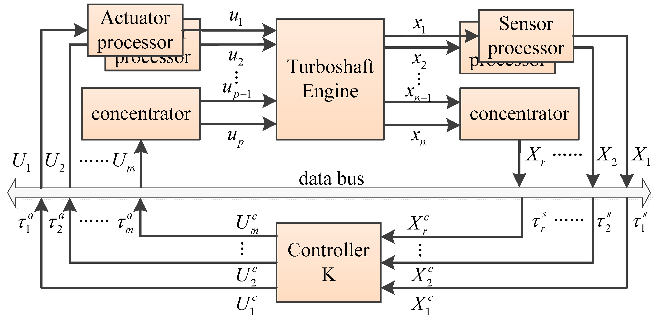
Although it has been developed for decades, there is no final conclusion on the structure of the DECSs [20], which is a gradual process from a centralized structure to a fully distributed structure. A partially distributed turboshaft engine control system architecture with concentrators and smart processor nodes is adopted in this paper; the schematic is shown in Figure 1 [21].

Figure 1 presents a DECS consisting of a turboshaft engine with n states, p inputs and q outputs and a state feedback controller. All these parameters are sensed or actuated by concentrators and processor nodes which are physically separated and attached across a shared data bus. The system with uncertainty for DECS is presented as:

$$\begin{array}{l}\{\begin{array}{l}\dot{x}\left(t\right)=\left[A+\Delta A\left(t\right)\right]x\left(t\right)+\left[B+\Delta B\left(t\right)\right]u\left(t\right)\\ x\left(t\right)=\varphi \left(t\right),t\le 0\\ u^c\left(t\right)=K{x}^c\left(t\right)\end{array}\end{array}$$

(1)

where $x\left(t\right)\in R^n$, $u\left(t\right)\in R^p$ are the state vector and control input vector, respectively; $x^c\left(t\right)$ is the delayed version of state vector, $u^c\left(t\right)$ is the version of control signal before the delay; $\varphi \left(t\right)$ is a continuously differentiable initial function; $A$ and $B$ are constant parameter matrices with appropriate dimensions, $K$ is the controller gain matrix; $\Delta A\left(t\right)$ and $\Delta B\left(t\right)$ denote the norm-bounded parameter uncertainties satisfying the following condition

$$\left[\begin{array}{cc}\Delta A& \Delta B\end{array}\right]=GF\left(t\right)\left[\begin{array}{cc}{E}_a& E_b\end{array}\right]$$

(2)

where $G$, $E_a$ and $E_b$ are constant matrices of appropriate dimension and $F\left(t\right)$ is an unknown time-varying matrix, which is Lebesgue measurable in t and satisfies $F^T\left(t\right)$$F\left(t\right)$ ≤ $I$.

Associated with system in Equation (1), the cost function is defined as:

$$J={\displaystyle {\int }_0^{\infty }\left[x^T\left(t\right)Qx\left(t\right)+u^T\left(t\right)Ru\left(t\right)\right]dt}$$

(3)

where $Q$ and $R$ are given positive-definite symmetric matrices. Also, according to the definition of the guaranteed cost control [22,23], the objective of the guaranteed cost controller design is to design a control law $u*\left(t\right)$ to minimize the upper bound of the cost function.

Throughout this paper, we assume that the sensors and controller are clock-driven and the actuators are event-driven. These nodes hold the latest data when packet dropout happened via zero-order-holders. The sensors and actuator have the same period denote as T, but they are triggered at different times. The actuators will respond immediately after receiving the control input. The time delay system method is used to model the system with multiple delays and packet dropouts [12,24,25,26].

For the DECS in Figure 1, the plant states are split into r parts

$$x\left(t\right)={\left[\begin{array}{ccc}{x}_1^T\left(t\right)& \cdots & x_r^T\left(t\right)\end{array}\right]}^T$$

(4)

and every part with its time stamp is lumped into one packet and transmitted in one channel and the time delay is ${\tau }_i^s\left(i=1,2,\dots ,r\right)$. Similarly, the control signals are split into $m$ parts

$$u^c\left(t\right)={\left[\begin{array}{ccc}{u}_1^c{\left(t\right)}^T& \cdots & u_m^c{\left(t\right)}^T\end{array}\right]}^T$$

(5)

and every part with its time stamp is also lumped into one packet, and the time delay is ${\tau }_j^a\left(j=1,2,\dots ,m\right)$ (including controller calculation time). In Equations (4) and (5), $x_i\left(t\right)\in R^{r_i}$ $,r_i\in Z^{+},{\displaystyle \sum _{i=1}^r{r}_i}=n$, and $u_i^c\left(t\right)\in R^{m_i},m_i\in Z^{+},{\displaystyle \sum _{i=1}^m{m}_i}=p.$

Then, the real input $u\left(t\right)$ realized through a zero-order-holder in Equation (1) is a piecewise constant function contains $m$ parts. Taking the network induced delays and packet dropouts into consideration, the real control system can be modeled as

$$\begin{array}{c}\dot{x}\left(t\right)=\left(A+\Delta A\right)x\left(t\right)+\left[B+\Delta B\left(t\right)\right]{\displaystyle \sum _{j=1}^m{u}_j\left(t\right)},t\in \left[i_k^{j}T+{\tau }_{j,k}^a,i_{k+1}^{j}T+{\tau }_{j,k+1}^a\right)\hfill \\ u_j\left(t\right)=u_j^c\left(t-{\tau }_{j,k}^a\right)=D_j{u}^c\left(t-{\tau }_{j,k}^a\right)={\displaystyle \sum _{i=1}^r{D}_{j}K{C}_i{x}^c\left(t-{\tau }_{j,k}^a-{\tau }_{i,k}^s\right)},t\in \left\{i_k^{j}T+{\tau }_{j,k}^a,k=1,2,\dots \right\}\hfill \end{array}$$

(6)

where $C_i=diag\left\{\begin{array}{ccc}\underset{i}{\underbrace{\begin{array}{ccc}0& \cdots & I_{r_i}\end{array}}}& \cdots & 0\end{array}\right\}$ and $D_j=diag\left\{\begin{array}{ccc}\underset{j}{\underbrace{\begin{array}{ccc}0& \cdots & I_{m_j}\end{array}}}& \cdots & 0\end{array}\right\}$; $i_k^j,k=1,2,\dots$ are some integers and $\left\{i_1^j,i_2^j,\dots \right\}\subset \left\{0,1,2,\dots \right\}$ and $i_k^{j}T$ denotes the instant the controller is triggered. From the above, we have

$$u\left(t\right)={\displaystyle \sum _{j=1}^m{\displaystyle \sum _{i=1}^r{D}_{j}K{C}_{i}x\left(t-{\tau }_{ij}\left(t\right)\right)}}$$

(7)

where ${\tau }_{ij}\left(t\right)={\tau }_{i,k}^s+{\tau }_{j,k}^a$. Then, it is also assumed that the pair $(A,B)$ in Equation (1) is stabilizable, and there exist constants $h_{1,ij},h_{2,ij}$ such that

$$\begin{array}{ccc}0<h_{1,ij}\le {\tau }_{ij}\left(t\right)\le h_{2,ij}& \forall i=1,2,\dots ,r& j=1,2,\dots ,m\end{array}$$

(8)

Denoting $h=ma{x}_1{}_{\le i\le r,1\le j\le m}\left\{h_{2,ij}\right\}$, then the model of NECSs with multiple delays under above assumptions can be described as follows:

$$\{\begin{array}{l}\dot{x}\left(t\right)=\left(A+\Delta A\right)x\left(t\right)+{\displaystyle \sum _{l=1}^s\left(B+\Delta B\right)K_{l}x\left(t-{\tau }_l\left(t\right)\right)}\\ x\left(t\right)=\varphi \left(t\right),t\in \left[-h,0\right],h_{1l}\le {\tau }_l\left(t\right)\le h_{2l},l=1,2,\dots ,s\end{array}$$

(9)

where

$$\begin{array}{l}{K}_l=D_{j}K{C}_i,{\tau }_l\left(t\right)={\tau }_{ij}\left(t\right),h_{1l}=h_{1,ij},h_{2l}=h_{2,ij}\le h,\\ \forall l=\left(j-1\right)\times r+i,i=1,2,\dots ,r;j=1,2,\dots ,m;s=r\times m,\end{array}$$

(10)

and Equation (3) can be rewritten as

$$J={\displaystyle {\int }_0^{\infty }\left[x^T\left(t\right)Qx\left(t\right)+{\left({\displaystyle \sum _{l=1}^s{K}_{l}x\left(t-{\tau }_l\left(t\right)\right)}\right)}^{T}R{\displaystyle \sum _{l=1}^s{K}_{l}x\left(t-{\tau }_l\left(t\right)\right)}\right]}dt$$

(11)

Remark 1.

The model of DECSs with multiple delays established above is same as the model in Reference [26] when$s=1$. So, the model of this paper includes the one of Reference [26] as a special case.

3. Guaranteed Cost Controller Design Method and Turboshaft Engine Modeling

In this section, the main methods used in the paper are shown. Section 3.1 presents a guaranteed cost controller design method and an iterative solve algorithm is given. Section 3.2 presents a turboshaft engine model with aging and deteriorations.

3.1. Guaranteed Cost Controller Design Method

Theorem 1.

For given scalars$h_{1l},h_{2l}$and${\gamma }_l\in \left[0,1\right]\left(l=1,2,\dots ,s\right)$and matrices$U_1$,$Q>0$and$R>0$, if there exist symmetric positive definite matrices$\overline{P},{\overline{Q}}_{1l},{\overline{Q}}_{2l},{\overline{Q}}_{3l},{\overline{R}}_{1l},{\overline{R}}_{2l},{\overline{R}}_{3l},{\overline{R}}_{4l},{\overline{R}}_{5l},{\overline{R}}_{6l}$, matrices$F_i,{\overline{X}}_l,{\overline{Y}}_l\left(l=1,2,\dots ,s\right)$and symmetric matrix${\overline{M}}_2$with appropriate dimension and scalar$\epsilon >0$, such that the LMIs Equations (12) and (13) hold, then$u\left(t\right)=Kx\left(t\right)$with$K=\left({\displaystyle \sum _{i=1}^r{F}_i}\right){\overline{M}}_2^{-1}$is a guaranteed cost controller.

$${\Phi }^{\left(1\right)}=\left[\begin{array}{cc}{\Phi }_{11}^{\left(1\right)}& {\Phi }_{12}^{\left(1\right)}\\ \ast & {\Phi }_{22}^{\left(1\right)}\end{array}\right]<0,{\Phi }^{\left(2\right)}=\left[\begin{array}{cc}{\Phi }_{11}^{\left(2\right)}& {\Phi }_{12}^{\left(2\right)}\\ \ast & {\Phi }_{22}^{\left(2\right)}\end{array}\right]<0$$

(12)

$$\left[\begin{array}{cc}{\overline{\Xi }}_{31,l}& {\overline{X}}_l\\ \ast & {\overline{\Xi }}_{31,l}\end{array}\right]>0,\left[\begin{array}{cc}{\overline{\Xi }}_{32,l}& {\overline{Y}}_l\\ \ast & {\overline{\Xi }}_{32,l}\end{array}\right]>0$$

(13)

where${\Phi }_{11}^{\left(1\right)},{\Phi }_{12}^{\left(1\right)},{\Phi }_{22}^{\left(1\right)},{\Phi }_{11}^{\left(2\right)},{\Phi }_{12}^{\left(2\right)},{\Phi }_{22}^{\left(2\right)},{\overline{\Xi }}_{31,l}$and${\overline{\Xi }}_{32,l}$are defined in Appendix A. At the same time the cost function$J^{\ast }$satisfies

$$J\le J_{11}+{\displaystyle \sum _{l=1}^s\left(J_{2l}+J_{3l}+J_{4l}+J_{5l}+J_{6l}+J_{7l}+J_{8l}+J_{9l}+J_{10l}\right)}=J^{\ast }$$

(14)

where

$$\begin{array}{c}{J}_{11}=x_0^T{\overline{M}}_2^{-T}\overline{P}{\overline{M}}_2^{-1}{x}_0,J_{2l}={\displaystyle {\int }_{-{\tau }_{1l}}^0{\phi }^T\left(\alpha \right){\overline{M}}_2^{-T}{\overline{Q}}_{1l}{\overline{M}}_2^{-1}\phi \left(\alpha \right)d\alpha },J_{3l}={\displaystyle {\int }_{-{\tau }_{ml}}^{-{\tau }_{1l}}{\phi }^T\left(\alpha \right){\overline{M}}_2^{-T}{\overline{Q}}_{2l}{\overline{M}}_2^{-1}\phi \left(\alpha \right)d\alpha },\hfill \\ J_{4l}={\displaystyle {\int }_{-{\tau }_{2l}}^{-{\tau }_{ml}}{\phi }^T\left(\alpha \right){\overline{M}}_2^{-T}{\overline{Q}}_{3l}{\overline{M}}_2^{-1}\phi \left(\alpha \right)d\alpha },J_{5l}={\tau }_{1l}{\displaystyle {\int }_{-{\tau }_{1l}}^0{\displaystyle {\int }_{\theta }^0{\dot{\phi }}^T\left(\alpha \right){\overline{M}}_2^{-T}{\overline{R}}_{1l}{\overline{M}}_2^{-1}\dot{\phi }\left(\alpha \right)d\alpha d\theta }},\hfill \\ J_{6l}=\left({\tau }_{ml}-{\tau }_{1l}\right){\displaystyle {\int }_{-{\tau }_{ml}}^{-{\tau }_{1l}}{\displaystyle {\int }_{\theta }^t{\dot{\phi }}^T\left(\alpha \right){\overline{M}}_2^{-T}{\overline{R}}_{2l}{\overline{M}}_2^{-1}\dot{\phi }\left(\alpha \right)d\alpha d\theta }},J_{7l}=\left({\tau }_{2l}-{\tau }_{ml}\right){\displaystyle {\int }_{-{\tau }_{2l}}^{-{\tau }_{ml}}{\displaystyle {\int }_{\theta }^t{\dot{\phi }}^T\left(\alpha \right){\overline{M}}_2^{-T}{\overline{R}}_{3l}{\overline{M}}_2^{-1}\dot{\phi }\left(\alpha \right)d\alpha d\theta }},\hfill \\ J_{8l}={\tau }_{1l}{\displaystyle {\int }_{-{\tau }_{1l}}^0{\displaystyle {\int }_{\theta }^0{\phi }^T\left(\alpha \right){\overline{M}}_2^{-T}{\overline{R}}_{4l}{\overline{M}}_2^{-1}\phi \left(\alpha \right)d\alpha d\theta }},J_{9l}=\left({\tau }_{ml}-{\tau }_{1l}\right){\displaystyle {\int }_{-{\tau }_{ml}}^{-{\tau }_{1l}}{\displaystyle {\int }_{\theta }^0{\phi }^T\left(\alpha \right){\overline{M}}_2^{-T}{\overline{R}}_{5l}{\overline{M}}_2^{-1}\phi \left(\alpha \right)d\alpha d\theta }},\hfill \\ J_{10l}=\left({\tau }_{2l}-{\tau }_{ml}\right){\displaystyle {\int }_{-{\tau }_{2l}}^{-{\tau }_{ml}}{\displaystyle {\int }_{\theta }^0{\phi }^T\left(\alpha \right){\overline{M}}_2^{-T}{\overline{R}}_{6l}{\overline{M}}_2^{-1}\phi \left(\alpha \right)d\alpha d\theta }}.\hfill \end{array}$$

Proof. 

The proof of Theorem 1 is given in Appendix B.□

For given scalars and matrices, in order to obtain a controller gain $K$ which achieves the least guaranteed cost value $J^{\ast }$, we have to solve the following minimization problem

$$\begin{array}{ccccc}Minimize& \left(14\right)& subject& to& \left(12\right),\left(13\right)\end{array}$$

(15)

However, it is noted that the terms in Equation (14) are not convex functions. As a result, we cannot find the general global minimum of the above minimization problem using a convex optimization algorithm. In order to get the upper bound of the cost function [22], we introduce some matrix values ${\Pi }_1,{\Pi }_{kl}\left(k=2,3,\dots 10,l=1,2,\dots ,s\right)$, such that

$$\begin{array}{c}{\Pi }_1=x_0{x}_0^T,{\Pi }_{2l}={\displaystyle {\int }_{-{\tau }_{1l}}^0\phi \left(\alpha \right){\phi }^T\left(\alpha \right)d\alpha },{\Pi }_{3l}={\displaystyle {\int }_{-{\tau }_{ml}}^{-{\tau }_{1l}}\phi \left(\alpha \right){\phi }^T\left(\alpha \right)d\alpha },{\Pi }_{4l}={\displaystyle {\int }_{-{\tau }_{2l}}^{-{\tau }_{ml}}\phi \left(\alpha \right){\phi }^T\left(\alpha \right)d\alpha },\hfill \\ {\Pi }_{5l}={\tau }_{1l}{\displaystyle {\int }_{-{\tau }_{1l}}^0{\displaystyle {\int }_{\theta }^0\dot{\phi }\left(\alpha \right){\dot{\phi }}^T\left(\alpha \right)d\alpha d\theta }},{\Pi }_{6l}=\left({\tau }_{ml}-{\tau }_{1l}\right){\displaystyle {\int }_{-{\tau }_{ml}}^{-{\tau }_{1l}}{\displaystyle {\int }_{\theta }^t\dot{\phi }\left(\alpha \right){\dot{\phi }}^T\left(\alpha \right)d\alpha d\theta }},\hfill \\ {\Pi }_{7l}=\left({\tau }_{2l}-{\tau }_{ml}\right){\displaystyle {\int }_{-{\tau }_{2l}}^{-{\tau }_{ml}}{\displaystyle {\int }_{\theta }^t\dot{\phi }\left(\alpha \right){\dot{\phi }}^T\left(\alpha \right)d\alpha d\theta }},{\Pi }_{8l}={\tau }_{1l}{\displaystyle {\int }_{-{\tau }_{1l}}^0{\displaystyle {\int }_{\theta }^0\phi \left(\alpha \right){\phi }^T\left(\alpha \right)d\alpha d\theta }},\hfill \\ {\Pi }_{9l}=\left({\tau }_{ml}-{\tau }_{1l}\right){\displaystyle {\int }_{-{\tau }_{ml}}^{-{\tau }_{1l}}{\displaystyle {\int }_{\theta }^0\phi \left(\alpha \right){\phi }^T\left(\alpha \right)d\alpha d\theta }},{\Pi }_{10l}=\left({\tau }_{2l}-{\tau }_{ml}\right){\displaystyle {\int }_{-{\tau }_{2l}}^{-{\tau }_{ml}}{\displaystyle {\int }_{\theta }^0\phi \left(\alpha \right){\phi }^T\left(\alpha \right)d\alpha d\theta }}.\hfill \end{array}$$

(16)

Let us introduce new variables ${\Lambda }_1={\Lambda }_1^T,{\Lambda }_{kl}={\Lambda }_{kl}^T\left(k=2,3,\dots ,10,l=1,2,\dots s\right)$ such that

$${\overline{M}}_2^{-T}\overline{P}{\overline{M}}_2^{-1}<{\Lambda }_1,{\overline{M}}_2^{-T}{\overline{Q}}_{g_{1}l}{\overline{M}}_2^{-1}<{\Pi }_{\left(g_1+1\right)l},{\overline{M}}_2^{-T}{\overline{R}}_{g_{2}l}{\overline{M}}_2^{-1}<{\Pi }_{\left(g_2+4\right)l},$$

(17)

By Schur complement and denoting $\widehat{P}={\overline{P}}^{-1},M_2={\overline{M}}_2^{-1},{\widehat{Q}}_{g_{1}l}={\overline{Q}}_{g_{1}l}^{-1},{\widehat{R}}_{g_{2}l}={\overline{R}}_{g_{2}l}^{-1}$, Equation (17) is equivalent to

$$\begin{array}{l}\left[\begin{array}{cc}-{\Lambda }_1& M_2^T\\ M_2& -\widehat{P}\end{array}\right]<0,\left[\begin{array}{cc}-{\Lambda }_{\left(g_1+1\right)l}& M_2^T\\ M_2& -{\widehat{Q}}_{g_{1}l}\end{array}\right]<0,\left[\begin{array}{cc}-{\Lambda }_{\left(g_2+4\right)l}& M_2^T\\ M_2& -{\widehat{R}}_{g_{2}l}\end{array}\right]<0,\\ \left(g_1=1,2,3;g_2=1,2,\dots ,6;k=2,3,\dots 10;l=1,2,\dots ,s\right)\end{array}$$

(18)

Then, the following inequalities hold

$$J_1<trace\left({\Pi }_1{\Lambda }_1\right),J_{kl}<trace\left({\Pi }_{kl}{\Lambda }_{kl}\right).$$

(19)

For some constant J, assuming

$$trace\left({\Pi }_1{\Lambda }_1\right)+{\displaystyle \sum _{k=2}^{10}{\displaystyle \sum _{l=1}^{s}trace\left({\Pi }_{kl}{\Lambda }_{kl}\right)}}<J$$

(20)

Combining these facts, we can construct a feasibility problem as follows:

Find $\begin{array}{l}\overline{P},\widehat{P},M_2,{\overline{M}}_2,{\overline{Q}}_{g_{1}l},{\widehat{Q}}_{g_{1}l},{\overline{R}}_{g_{2}l},{\widehat{R}}_{g_{2}l},{\Lambda }_1,{\Lambda }_{kl},{\overline{X}}_l,{\overline{Y}}_l,F_i,\epsilon \\ (g_1=1,2,3;g_2=1,2,\dots ,6;i=1,2,\dots ,r;l=1,2,\dots ,s)\end{array}$

Subject to $\overline{P}>0,{\overline{Q}}_{g_{1}l}>0,{\overline{R}}_{g_{2}l}>0,\epsilon >0,\widehat{P}={\overline{P}}^{-1},M_2={\overline{M}}_2^{-1},{\widehat{Q}}_{g_{1}l}={\overline{Q}}_{g_{1}l}^{-1},{\widehat{R}}_{g_{2}l}={\overline{R}}_{g_{2}l}^{-1},\left(12\right),\left(13\right),\left(18\right),\left(20\right).$

Because there are nonlinear constraints, such as $\widehat{P}={\overline{P}}^{-1}$ et al., the feasibility problem is still difficult to solve. These nonlinear constraints can be linearized via the cone complementarity linearization algorithm [22,27]. Then, the feasibility problem can be transformed into a minimization problem with LMI constraints:

$\begin{array}{cc}Minimize& trace\left(M_2{\overline{M}}_2+\overline{P}\widehat{P}+{\displaystyle \sum _{g_1=1}^3{\displaystyle \sum _{l=1}^s{\overline{Q}}_{g_{1}l}{\widehat{Q}}_{g_{1}l}}+}{\displaystyle \sum _{g_2=1}^6{\displaystyle \sum _{l=1}^s{\overline{Q}}_{g_{2}l}{\widehat{Q}}_{g_{2}l}}}\right)\end{array}$

Subject to

$$\begin{array}{l}\overline{P}>0,{\overline{Q}}_{g_{1}l}>0,{\overline{R}}_{g_{2}l}>0,\left(12\right),\left(13\right),\left(18\right),\left(20\right)\\ \left[\begin{array}{cc}{M}_2& I\\ I& {\overline{M}}_2\end{array}\right]\ge 0,\left[\begin{array}{cc}\overline{P}& I\\ I& \widehat{P}\end{array}\right]\ge 0,\left[\begin{array}{cc}{\overline{Q}}_{g_{1}l}& I\\ I& {\widehat{Q}}_{g_{1}l}\end{array}\right]\ge 0,\left[\begin{array}{cc}{\overline{R}}_{g_{2}l}& I\\ I& {\widehat{R}}_{g_{2}l}\end{array}\right]\ge 0\\ g_1=1,2,3;g_2=1,2,\dots ,6;l=1,2,\dots ,s.\end{array}$$

(21)

Based on this cone complementarity problem and the solving algorithm in references [19,27], the least upper bound of the cost function can be solved iteratively. The iterative algorithm starts with a sufficiently large $J$ in Equation (20), and then decreases the value of $J$ continuously until the above optimization problem has no solution, at which point the least upper bound of cost function is obtained.

Although it is still impossible to always find the globally optimal solution, the proposed linear optimization problem is easier to solve than the original non-convex minimization problem in Equation (14).

3.2. Modeling of Turboshaft Engine with Aging and Deterioration

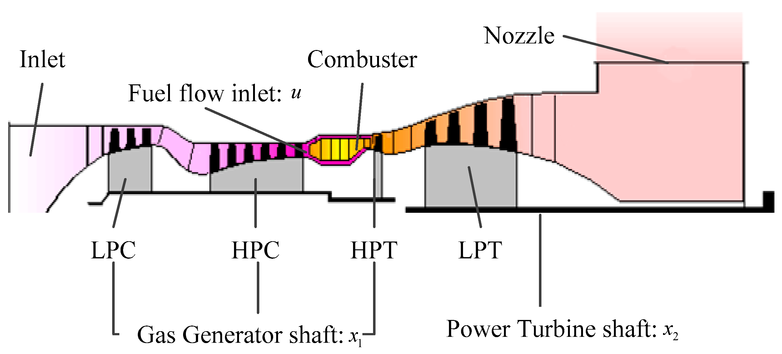
A typical turboshaft engine consists of two parts: a gas generator and power turbine. The gas generator consists of a low-pressure compressor, a high-pressure compressor, a combustion chamber and a gas generator turbine [28]. It is used to generate the high temperature and pressure gas to drive the independent power turbine. Then, the power turbine is used to drive the load link to the turbine shaft. The primary components of a typical turboshaft engine are shown in Figure 2. The aim of the turboshaft engine control, therefore, is to keep the power turbine at a constant speed [29].

In reference [30], using GasTurb modeling software [31], a versatile simulation platform for turboshaft engine control system is established. With this platform, we can flexibly generate a turboshaft linear model with customized structures and characteristics at a design point. The design point taken for this paper is 100% gas generator speed and 100% power turbine speed with an altitude of 0 and Mach number of 0.

Table 1. Parameters and physical meanings of the turboshaft engine model.

Signal Type	Notation	Designed Value	Physical Meanings
Input	u	0.1356 Kg/min	Main combustor fuel flow
State vector x	x1	37800 rpm	Rotation speed of the gas generator
	x2	20900 rpm	Rotation speed of the power turbine
Output y	y	20900 rpm	Being same as x2
Health parameter w	w1	1.00	Efficiency modifier of the low-pressure compressor
	w2	1.00	Efficiency modifier of the high-pressure compressor
	w3	1.00	Efficiency modifier of the gas generator turbine
	w4	1.00	Efficiency modifier of the power turbine
	w5	1.00	Flow modifier of the low-pressure compressor
	w6	1.00	Flow modifier of the high-pressure compressor
	w7	1.00	Flow modifier of the gas generator turbine
	w8	1.00	Flow modifier of the power turbine

shows the state vector $x$, input $u$, the output $y$ and the health parameter vector w for a new turboshaft at the design point.

As an engine is used, degradation happens, which yields a shorter life and higher cost. Usually, the degradation is reflected as changes in flow characteristics and efficiencies of the rotational components. Therefore, a group of multipliers called “health parameters” are introduced in the model. For example, w_i = 1 (i=1, 2, …, 8) stands for a new component while w_i ≠ 1 stands for a degraded one, in which the flow modifiers for turbines (w₇ and w₈) increase, and other parameters (w₁ to w₆) decrease. In this paper, the health parameter settings are borrowed from reference [32].

By way of the versatile simulation platform and manipulating the flow modifiers w₇ and w₈ from 1 to 1.025 and other health parameters (w₁ to w₆) from 1 to 0.975 at 0.005 intervals, we can get a set of the turboshaft engine linear models at the design point. The models are identified as

$$\{\begin{array}{l}\delta \dot{x}\left(t\right)={𝒜}_j\cdot \delta x\left(t\right)+{ℬ}_j\cdot \delta u\left(t\right)\\ \delta y\left(t\right)={𝒞}_j\cdot \delta x\left(t\right)+{𝒟}_j\cdot \delta u\left(t\right)\\ j=1,2,\dots ,6\end{array}$$

(22)

where the symbol $\delta$ denotes the deviation from the design point, and the parameter matrices of the models constitute the set $ℒ$:

$$ℒ\triangleq \left\{L|L=\left[\begin{array}{cc}{𝒜}_j& {ℬ}_j\\ {𝒞}_j& {𝒟}_j\end{array}\right],j=1,2,\dots ,6\right\}$$

(23)

Then, based on Lemma 1 in reference [11,33], Corollary 1 is derived as follows.

Corollary 1.

With the given matrices$P\triangleq {\left(p_{ij}\right)}_{n\times m}$,$Q\triangleq {\left(q_{ij}\right)}_{n\times m}$and$𝒜\triangleq {\left(a_{ij}\right)}_{n\times m}$, the interval matrix$𝒩\left[P,Q\right]$is equivalent to the set${ℳ}_a$defined below:

$${ℳ}_a\triangleq \left\{𝒜\in R^{n\times m}|𝒜=A+G_a{F}_a{E}_a,F_a^T{F}_a\le I\right\}$$

(24)

where the interval is defined as

$${ℳ}_a\triangleq \left\{𝒜\in R^{n\times m}|𝒜=A+G_a{F}_a{E}_a,F_a^T{F}_a\le I\right\}$$

(25)

$$\begin{array}{l}\mathit{\text{and matrices }}{G}_a\in R^{n\times nm},F_a\in R^{nm\times nm}\mathit{\text{ and }}{E}_a\in R^{nm\times m}\mathit{\text{ are taken as}}\hfill \\ A=\frac{P+Q}{2},H={\left(H_{ij}\right)}_{n\times m}=\frac{Q-P}{2},\hfill \\ G_a=\left[\begin{array}{ccccccc}\sqrt{h_{11}}{e}_1& \cdots & \sqrt{h_{1m}}{e}_1& \cdots & \sqrt{h_{n1}}{e}_n& \cdots & \sqrt{h_{nm}}{e}_n\end{array}\right],\hfill \\ E_a={\left[\begin{array}{ccccccc}\sqrt{h_{11}}{e}_1& \cdots & \sqrt{h_{1m}}{e}_m& \cdots & \sqrt{h_{n1}}{e}_1& \cdots & \sqrt{h_{nm}}{e}_m\end{array}\right]}^T,\hfill \\ e_k={\left[\underset{k}{\underbrace{0,\dots ,0,1}},0,\dots ,0\right]}^T,\left(k\in Z^{+}\right),\hfill \\ F_a=diag\left({\epsilon }_{11},\cdots {\epsilon }_{1m},\cdots ,{\epsilon }_{n1},\cdots ,{\epsilon }_{nm}\right),\left|{\epsilon }_{ij}\right|\le 1,i=1,2,\dots ,n;j=1,2,\dots ,m.\hfill \end{array}$$

Remark 2.

The equivalence of$𝒩\left[P,Q\right]$and${ℳ}_a$for square matrix has been proved in Reference [33], here we generalize it to more general non-square matrix and the proof process is similar to the reference and is omitted here.

Then, degradation of the health parameters w is viewed as the source of uncertainties for the identified models. Taking all parameter matrices in Equation (23) into Corollary 1, we can get the parameter matrices of turboshaft engine at design point with norm-bounded uncertainties.

$$ℳ\triangleq \left\{M|M=\left[\begin{array}{cc}A& B\\ C& D\end{array}\right]+\left[\begin{array}{cc}{G}_a{F}_a{E}_a& G_b{F}_b{E}_b\\ G_c{F}_c{E}_c& G_d{F}_d{E}_d\end{array}\right],F_i^T{F}_i\le I,i\in \left\{a,b,c,d\right\}\right\}$$

(26)

where

$$\begin{array}{l}A=\left[\begin{array}{cc}-3.9519& -0.0524\\ 0.5239& -1.2656\end{array}\right],G_a=\left[\begin{array}{cccc}0.1560& 0.0383& 0& 0\\ 0& 0& 0.1538& 0.0716\end{array}\right],E_a=\left[\begin{array}{cc}0.1560& 0\\ 0& 0.0383\\ 0.1538& 0\\ 0& 0.0716\end{array}\right],\\ B=\left[\begin{array}{c}1.0788\\ 0.3116\end{array}\right],G_b=\left[\begin{array}{cc}0.2118& 0\\ 0& 0.0526\end{array}\right],E_b=\left[\begin{array}{c}0.2118\\ 0.0526\end{array}\right],\\ C=\left[\begin{array}{cc}0& 1\end{array}\right],G_c=\left[\begin{array}{cc}0& 0\end{array}\right],E_c=0_{2\times 2},D=0,G_d=0,E_d=0.\end{array}$$

Therefore, a group of turboshaft engine linear models at design point in Equation (23) with aging and deterioration are rewritten as nominal model in Equation (26) with norm-bounded uncertainties.

Remark 3.

Since the model set$ℒ$is only a subset of norm-bounded uncertainties model$ℳ$, the conservatism is introduced.

It should be noticed that the steady-state error may exist in the control system with static state feedback controller. This error can be eliminated by achieving the integral action via internal model principle [34,35]. The turboshaft engine control system can be augmented as

$$\{\begin{array}{l}\dot{\overline{x}}\left(t\right)=\overline{𝒜}\overline{x}\left(t\right)+\overline{ℬ}\overline{u}\left(t\right)\\ {\overline{u}}^c\left(t\right)=K{\overline{x}}^c\left(t\right)\end{array}$$

(27)

where $\overline{x}\triangleq {\left[{\begin{array}{cc}\delta x^T& z\end{array}}^T\right]}^T$, $z\triangleq {\displaystyle \int \left[\delta y_{cmd}-\delta y\left(t\right)\right]dt}$. The turboshaft engine control system is a constant speed control system [29,36], so $\delta y_{cmd}\equiv 0$ is always true. $\overline{𝒜}$ and $\overline{ℬ}$ are augmented system matrices that can still be decomposed into a norm-bounded form as

$$\begin{array}{l}\overline{𝒜}=\overline{A}+\Delta \overline{A},\overline{ℬ}=\overline{B}+\Delta \overline{B},\\ \left[\Delta \overline{A}¦\Delta \overline{B}\right]=\overline{G}\overline{F}\left[{\overline{E}}_a¦{\overline{E}}_b\right]\end{array}$$

(28)

where

$\begin{array}{l}\overline{A}=\left[\begin{array}{cc}A& 0\\ -C& 0\end{array}\right],\overline{B}=\left[\begin{array}{c}B\\ -D\end{array}\right],\overline{G}=\left[\begin{array}{cccc}{G}_a& 0& G_b& 0\\ 0& G_c& 0& G_d\end{array}\right],{\overline{E}}_a={\left[\begin{array}{cccc}{E}_a& E_c& 0& 0\\ 0& 0& 0& 0\end{array}\right]}^T,{\overline{E}}_b={\left[\begin{array}{cccc}0& 0& E_b& E_d\end{array}\right]}^T,\\ \overline{F}=diag\left(F_a,-F_c,F_b,-F_d,\right).\end{array}$

However, the augmented state vector contains three variables: gas generator speed (N_g), power turbine speed (N_p) and integration of power turbine speed (z), only N_g and N_p are sensed and transmitted physically. So, the states are transmitted by two packets in state channels. Then, the controller design, the augmented state is divided into two parts—$X_1\left(t\right)=\delta x_1\left(t\right)$,$X_2\left(t\right)={\left[\begin{array}{cc}\delta x_2^T\left(t\right)& z^T\left(t\right)\end{array}\right]}^T$ and the r = 2 in Theorem 1. The control input is fuel flow (W_f) transmitted by one packet in the control channel, and m = 1 in Theorem 1.

4. Application and Simulations on the Turboshaft Engine DECS

This section presents the application of the method proposed, and four simulations are performed. The first numerical calculation shows that the method proposed is less conservative in comparison to references [19,24]. The second simulation shows that the method proposed is effective for multiple delays and packet dropouts. The third simulation shows that the guaranteed cost control is more robust than a legacy cascade PI controller for multiple delays and packet dropouts. The fourth simulation presents the robustness of the method for aging and deterioration.

In the DECSs, since a time-triggered data bus is utilized, the transmission delays are less than one sampling period $T=0.02\mathrm{s}$. We assume that the lower bounds of multiple delays are half period $h_{11}=h_{12}=0.01\mathrm{s}$, and the upper bounds of multiple delays are one period. The controller gain $K$ for the system with different delays/dropouts are upper bound and uncertainties are calculated for the augmented system by the method proposed.

Firstly, to illustrate that the method proposed is less conservative, we get a base LQR controller $K=\left[\begin{array}{ccc}3.6734& 23.8746& -88.4129\end{array}\right]$ at nominal point by setting $Q=diag(1,1,100)$ and $R=0.01$. When we assume that $h_{21}=h_{22}$ in two channels (namely, a single delay system), the maximum allowable value of $h_{21}$ and $h_{22}$ are obtained as 0.107 s by the method in this paper and setting ${\gamma }_1={\gamma }_2=0.38$. Correspondingly, the maximum value of $h_{21}$ and $h_{22}$ are 0.101 s by the method in references [19,24]. Then, for a multiple delay system, we fixed the value of $h_{21,max}=0.09$ s, the maximum allowable value of $h_{22}$ is obtained as 0.111 s by the method in this paper and setting ${\gamma }_1={\gamma }_2=0.42$. Correspondingly, the maximum value of $h_{22}$ is 0.108 s by using the method in references [19,24].

Then, to verify the effectiveness of the controller designed by the method proposed, we take

$$\begin{array}{l}\left[\begin{array}{cc}{h}_{21}& h_{22}\end{array}\right]\in \left\{{\left[\begin{array}{c}0.02\\ 0.02\end{array}\right]}^T,{\left[\begin{array}{c}0.12\\ 0.12\end{array}\right]}^T,{\left[\begin{array}{c}0.12\\ 0.22\end{array}\right]}^T,{\left[\begin{array}{c}0.22\\ 0.12\end{array}\right]}^T,{\left[\begin{array}{c}0.22\\ 0.22\end{array}\right]}^T\right\},\\ {\gamma }_1={\gamma }_2=0.38,U_1=0.1*I,Q=diag\left(1,1,100\right),R=0.01,{\overline{x}}^T\left(0\right)=\left[\begin{array}{ccc}-1.3\%x_{1,des}& 0& 0\end{array}\right],{\dot{\overline{x}}}^T\left(0^{-}\right)=0,\end{array}$$

(29)

where $h_{21}$ and $h_{22}$ denote upper bound of time delays and packet dropouts of two channels, subscript des means the designed point value and the initial value can be reached by setting the power angle from 100% to 95%. The guaranteed cost controller $K_{h_{21},h_{22}}$ and the least upper bound of cost functions $J_{min}$ for the system with different delays, packet dropouts and uncertainties are calculated and listed in

Table 2. Calculation results and performances of system with multiple delays and packet dropouts.

Situation No.	$\left[\begin{array}{cc}{\mathit{h}}_{21}& {\mathit{h}}_{22}\end{array}\right]$	${\mathit{K}}_{{\mathit{h}}_{21},{\mathit{h}}_{22}}$	${\mathit{J}}_{\mathit{m}\mathit{i}\mathit{n}}$$(\times {10}^{-3})$	Setting Time (s)	Fluctuation of Np (%)
1	$\left[\begin{array}{cc}0.02& 0.02\end{array}\right]$	$K_{0.02,0.02}=\left[\begin{array}{ccc}-0.9082& -5.4541& 4.3927\end{array}\right]$	6.5	2.78	−0.59
2	$\left[\begin{array}{cc}0.12& 0.12\end{array}\right]$	$K_{0.12,0.12}=\left[\begin{array}{ccc}-0.6877& -4.1765& 3.3489\end{array}\right]$	9.1	3.26	−0.69
3	$\left[\begin{array}{cc}0.12& 0.22\end{array}\right]$	$K_{0.12,0.22}=\left[\begin{array}{ccc}-0.7356& -4.3553& 3.5235\end{array}\right]$	9	3.10	−0.71
4	$\left[\begin{array}{cc}0.22& 0.12\end{array}\right]$	$K_{0.22,0.12}=\left[\begin{array}{ccc}-0.7174& -4.3014& 3.4805\end{array}\right]$	9.1	3.18	−0.67
5	$\left[\begin{array}{cc}0.22& 0.22\end{array}\right]$	$K_{0.22,0.22}=\left[\begin{array}{ccc}-0.5477& -3.3125& 2.7058\end{array}\right]$	11.8	3.66	−0.78
6	$\left[\begin{array}{cc}0.12& 0.22\end{array}\right]$	$K_{0.22,0.22}=\left[\begin{array}{ccc}-0.5477& -3.3125& 2.7058\end{array}\right]$	/*	3.66	−0.78

* The symbol ‘/’ means the controller for this simulation is not recalculated, so there is no corresponding cost function value J_min.

.

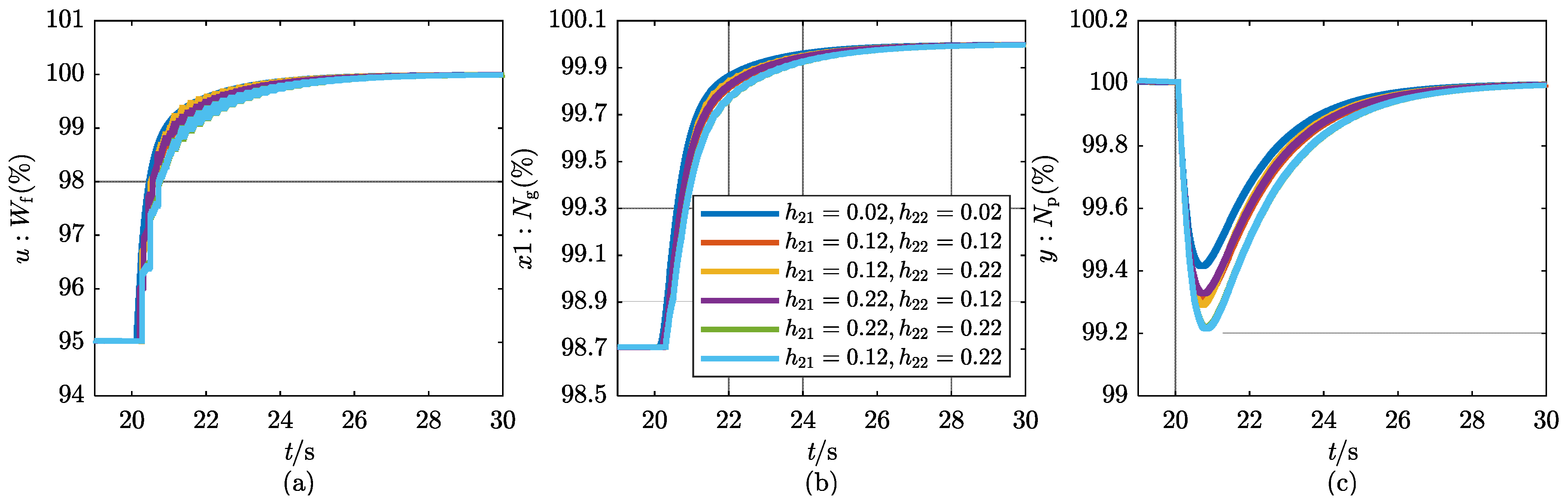
The simulations are performed on the turboshaft engine simulation platform, which is built based on the TrueTime toolbox [37]. During the simulation, we take the time delays as their worst values—which are one sampling period 0.02 s—and set the maximum consecutive packet dropouts of the two channels in DECS at n_1,max = {0,5,5,10,10,5} and n_2,max = {0,5,10,5,10,10}, corresponding situation 1 to situation 6. At the beginning of the simulations, the engine is driven to the initial status in Equation (29). Then, the power level angle changed from 95% to 100% again to make the whole system converge to its equilibrium point. The system response with delays and different packet dropouts are pictured in Figure 3, and dynamic performances are also listed in Table 2. All the data have been normalized by their designed point values to present in percentage.

As can be seen in Figure 3, the blue curve has the best performance, corresponding to the minimum delay and dropout (situation 1). The green curve (overlapped with the light blue curve) has the worst performance, corresponding to the maximum delay and dropout (situation 5). Simulation results from situation 1 to situation 5 show that with the increase in delays and dropouts, the performances of the guaranteed cost controller proposed will decrease, but it can still ensure the system remains stable. So, the controller design method proposed remains robust for multiple delays and packet dropouts. According to Table 2, we know that situation 3 and situation 6 have the same multiple delays and packet dropouts. However, in the simulations, situation 3 uses the multiple delay controller ($K_{0.12,0.22}$), and situation 6 uses the single delay controller ($K_{0.22,0.22}$). The result of situation 3 (yellow curve) is better than the result of situation 6 (light blue curve). So, for the practical multiple delay systems, the multiple delays controller is better than the single delay controller.

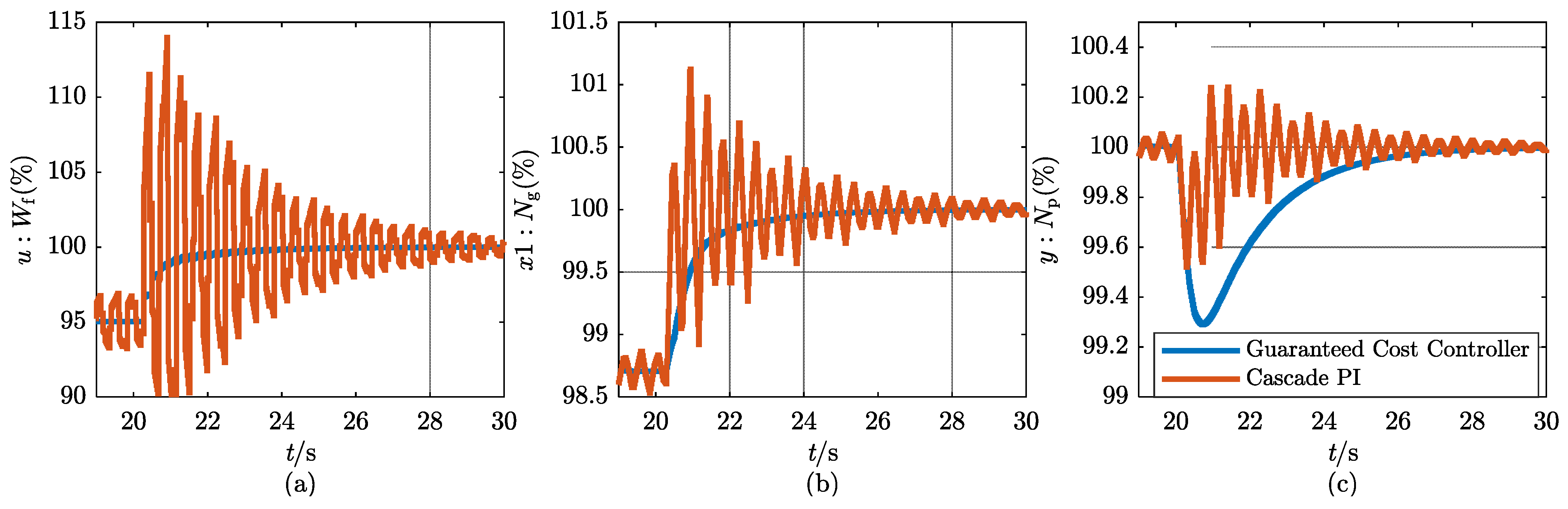
Thirdly, to compare the guaranteed cost controller proposed with the traditional cascade PI controller used in the turboshaft engine control system, we set the maximum delay of two channels as $\left[h_{21}{h}_{22}\right]=\left[0.120.22\right]$ and perform the simulations under the guaranteed cost controller and baseline cascade PI controller in the versatile simulation platform [30]. The controller parameters for inner loop are $K_{P1}=3.16\times {10}^{-5},K_{I1}=7.9\times {10}^{-5}$ and the controller parameters for outer loop are $K_{P2}=4.817,K_{I2}=10.44$, which are tuned by MATLAB SISO design toolbox with no uncertainties. During the simulation, the power level angle changed from 95% to 100% again to make the whole system converge to its equilibrium point. The responses are shown in Figure 4. Although from N_p we see that the cascade PI controller makes the system respond faster, the response oscillations of the system are more severe (orange curve). The guaranteed cost controller ensures stability and no oscillation for NECS with multiple delays and packet dropouts (blue curve). From the input W_f and gas generator speed N_g, we can see that the system under guaranteed cost control has faster responses. All of these show that the proposed guaranteed cost controller is more robust for multiple delays and packet dropouts, but the cost is that the drop-down amplitude of power turbine speed becomes worse.

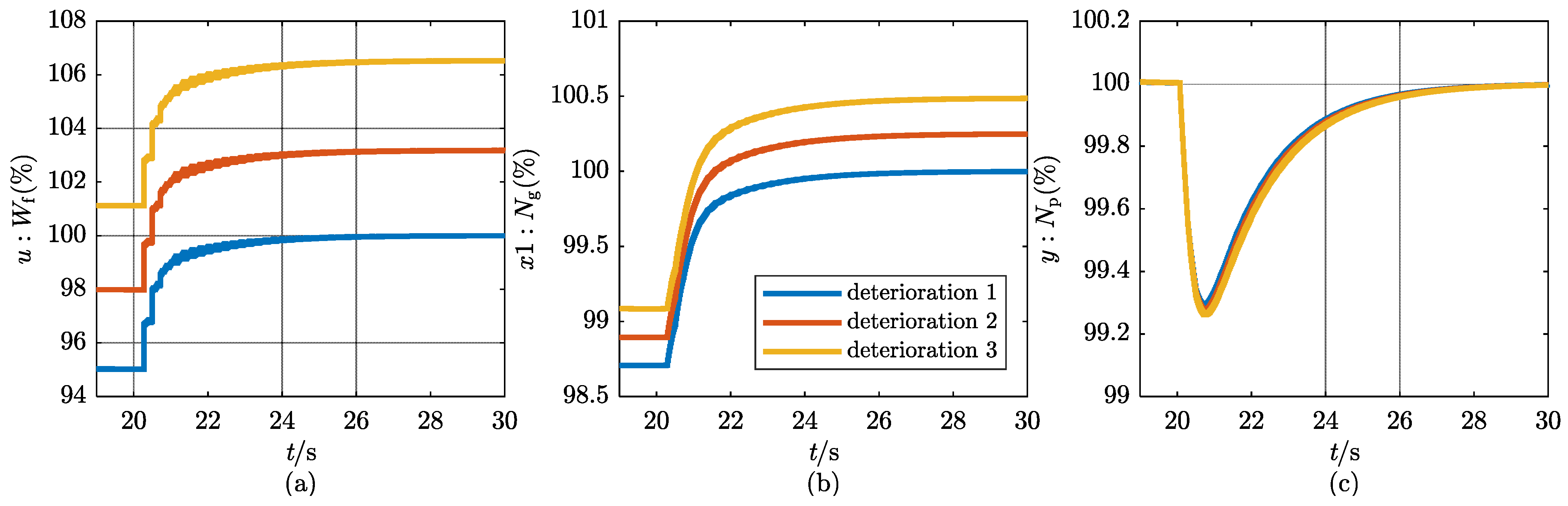
Finally, we confirm the robustness of the guaranteed cost controller designed for engine aging and deterioration by simulation. In each simulation, the $\left[h_{21}{h}_{22}\right]$ is fixed to [0.12 0.22], and the health parameters degrade in which the flow modifiers (w₇ and w₈) from 1 to 1.02 and other health parameters (w₁ to w₆) from 1 to 0.98 at 0.01 intervals. During the simulation, the power level angle changed from 95% to 100% again, to make the power turbine speed N_p converge to its equilibrium point. The system responses are pictured in Figure 5. From scenario 1 to scenario 3, engine deterioration became more and more severe. However, the guaranteed cost controller could still ensure the system was robust for multiple delays, packet dropouts and deterioration. The cost is that to keep the power turbine speed N_p at the desired constant value, more fuel W_f and higher gas generator speed N_g are needed. Also, this may cause fuel W_f and gas generator speed N_g to exceed the limits.

5. Conclusions

In this paper, a DECS with multiple-packet transmission delays and packet dropouts in both sensor channels, actuator channels and uncertainties is built. Then, a less conservative guaranteed cost controller design method is proposed using the LMI-based method. Finally, the method proposed is used to design controllers for the turboshaft engine distributed control system to deal with the problem of multiple delays and packet dropouts in the system, as well as the engine aging and deterioration. The simulations illustrate that the guaranteed cost controller proposed is robust for both a single delay system and multiple delay system, and the multiple delay controller performs better than the single delay controller for the turboshaft engine DECS. Also, the guaranteed cost controller designed is more robust than the cascade PI controller for multiple delays, and is effective for turboshaft engine aging and deterioration. This paper provides a design reference for the practical implementation of distributed engine control systems in the future.

References

1. Culley, D.; Thomas, R.; Saus, J. Concepts for distributed engine control. In Proceedings of the 43rd AIAA/ASME/SAE/ASEE Joint Propulsion Conference & Exhibit, Cincinnati, OH, USA, 8–11 July 2007. [Google Scholar] [CrossRef] [Green Version]
2. Culley, D.E.; Paluszewski, P.J.; Storey, W.; Smith, B.J. The Case for Distributed Engine Control in TurboShaft Engine Systems. In Proceedings of the 65th Annual Forum and Technology Display, Grapevine, TX, USA, 27–29 May 2009. [Google Scholar]
3. Yedavalli, R.K.; Belapurkar, R.K.; Behbahani, A. Design of Distributed Engine Control Systems for Stability Under Communication Packet Dropouts. J. Guido. Control. Dyn. 2009, 32, 1544–1549. [Google Scholar] [CrossRef]
4. Belapurkar, R.; Yedavalli, R.; Paluszewski, P. Design of set-point controller for partially distributed turboshaft engine with network faults. In Proceedings of the 47th AIAA/ASME/SAE/ASEE Joint Propultion Conference & Exhibit, San Diego, CA, USA, 31 July–3 August 2011. [Google Scholar] [CrossRef]
5. Pakmehr, M.; Chakravarthy Muralidhar, R.S.; Sutter, L.F.; Cohen, R.P.; Feron, E.M.; Behbahani, A.R. Developing Concepts for Optimal Scheduling in Distributed Turbine Engine Control Systems. In Proceedings of the AIAA Propulsion and Energy 2019 Forum, Indianapolis, IN, USA, 19–22 August 2019. [Google Scholar] [CrossRef]
6. Culley, D. Transition in Gas Turbine Control System Architecture: Modular, Distributed, and Embedded. In Proceedings of the Turbo Expo 2010, Glasgow, UK, 14–18 June 2010; pp. 287–297. [Google Scholar] [CrossRef] [Green Version]
7. Behbahani, A.; Culley, D.; Carpenter, S.; Mailander, B.; Hegwood, B.; Smith, B.; Darouse, C.; Mahoney, T.; Quinn, R.; Battestin, G.; et al. Status, Vision, and Challenges of an Intelligent Distributed Engine Control Architecture; SAE International Technical Report; SAE International: Warrendale, PA, USA, September 2007. [Google Scholar] [CrossRef] [Green Version]
8. Culley, D.; Behbahani, A. Communication Needs Assessments for Distributed Turbine Engine Control. In Proceedings of the 44th AIAA/ASME/SAE/ASEE Joint Propulsion Conference & Exhibit, Hartford, CT, USA, 21–23 July 2008. [Google Scholar] [CrossRef] [Green Version]
9. De Giorgi, M.; Strafella, L.; Ficarella, A. Neural Nonlinear Autoregressive Model with Exogenous Input (NARX) for Turboshaft Aeroengine Fuel Control Unit Model. Aerospace 2021, 8, 206. [Google Scholar] [CrossRef]
10. Lian, F.-L.; Moyne, J.; Tilbury, D. Performance evaluation of control networks: Ethernet, ControlNet, and DeviceNet. IEEE Control Syst. 2001, 21, 66–83. [Google Scholar] [CrossRef] [Green Version]
11. Li, R.; Nguang, S.K.; Guo, Y.; Chen, Y. Networked Control System Design for Turbofan Aeroengines with Aging and Deterioration. Complexity 2018, 2018, 1–13. [Google Scholar] [CrossRef]
12. Yue, D.; Han, Q.-L.; Lam, J. Network-based robust H∞ control of systems with uncertainty. Automatica 2005, 41, 999–1007. [Google Scholar] [CrossRef]
13. Nilsson, J. Real-Time Control Systems with Delays. Ph.D. Thesis, Lund Institute of Technology, Lund, Sweden, 11 February 1998. [Google Scholar]
14. Belapurkar, R.K. Stability and performance of propulsion control systems with distributed control architectures and failures. Ph.D. Thesis, The Ohio State University, Columbus, OH, USA, 2013. [Google Scholar]
15. Chen, Y.; Guo, Y.; Li, R. State Feedback Control for Partially Distributed Turboshaft Engine with Time Delay and Packet Dropouts. In Proceedings of the 37th Chinese Control Conference (CCC), Wuhan, China, 25–27 July 2018; pp. 9854–9859. [Google Scholar] [CrossRef]
16. Liu, X.; Sun, X. H Networked Cascade Control System Design for Turboshaft Engines with Random Packet Dropouts. Int. J. Aerosp. Eng. 2017, 2017, 1–12. [Google Scholar] [CrossRef]
17. Liu, X.; Luo, C. Stability Analysis for GE T700 Turboshaft Distributed Engine Control Systems. IEEE Access 2017, 5, 22485–22491. [Google Scholar] [CrossRef]
18. Seitz, T.; Yedavalli, R.; Macmann, O.; Behbahani, A. Robust Control of Turbine Engines Using Distributed Networks with Multiple Time Delays. J. Guid. Control. Dyn. 2017, 40, 2771–2781. [Google Scholar] [CrossRef]
19. Chen, Y.; Guo, Y.; Mao, H.; Li, R. Guaranteed Cost Controller Design for Distributed Engine Control System with Multiple Delay and Packet Losses. In Proceedings of the AIAA Propulsion and Energy 2020 Forum, Virtual Event, 24—28 August 2020. [Google Scholar] [CrossRef]
20. Popov, V.; Yepifanov, S.; Kononykhyn, Y.; Tsaglov, A. Architecture of Distributed Control System for Gearbox-Free More Electric Turbofan Engine. Aerospace 2021, 8, 316. [Google Scholar] [CrossRef]
21. Chen, Y.; Guo, Y.; Li, R.; Guo, L.; Han, T. Design of Turboshaft Engine Distributed Control System Architecture. Aeronautical Comp. Tech. 2019, 49, 21–26. [Google Scholar] [CrossRef]
22. Xie, J.-S.; Fan, B.-Q.; Young, S.L.; Yang, J. Guaranteed Cost Controller Design of Networked Control Systems with State Delay. Acta Autom. Sin. 2007, 33, 0171. [Google Scholar] [CrossRef] [Green Version]
23. Yu, L.; Chu, J. An LMI approach to guaranteed cost control of linear uncertain time-delay systems. Automatica 1999, 35, 1155–1159. [Google Scholar] [CrossRef]
24. Zhu, X.-L.; Yang, G.-H. Stability analysis and state feedback control of networked control systems with multi-packet transmission. In Proceedings of the American Control Conference, Seattle, WA, USA, 11–13 June 2008; pp. 3133–3138. [Google Scholar] [CrossRef] [Green Version]
25. Zhu, X.-L.; Yang, G.-H. State feedback controller design of networked control systems with multiple-packet transmission. Int. J. Control 2008, 82, 86–94. [Google Scholar] [CrossRef]
26. Yue, D.; Han, Q.-L.; Peng, C. State Feedback Controller Design of Networked Control Systems. IEEE Trans. Circuits Syst. II: Express Briefs 2004, 51, 640–644. [Google Scholar] [CrossRef]
27. El Ghaoui, L.; Oustry, F.; AitRami, M. A cone complementarity linearization algorithm for static output-feedback and related problems. IEEE Trans. Autom. Control 1997, 42, 1171–1176. [Google Scholar] [CrossRef] [Green Version]
28. Ballin, M.G. A High Fidelity Real-Time Simulation of a Small Turboshaft Engine; NASA Technical Memorandum: Moffett Field, CA, USA, 1 July 1988.
29. Delosreyes, G.; Gouchoe, D.R. The Design of a Turboshaft Speed Governor Using Modern Control Techniques; Contractor Report; NASA Lewis Research Center: Cleveland, OH, USA, 1 February 1986.
30. Mao, H.; Guo, Y.; Li, R.; Lai, C. Versatile Simulation Platform for Turboshaft Engine Control System. In Proceedings of the 2019 Chinese Control Conference, Guangzhou, China, 27–30 July 2019; pp. 7211–7216. [Google Scholar] [CrossRef]
31. Kurzke, J. GasTurb 11: Design and Off-Design Performance of Gas Turbines; GasTurb Gmbh: Aachen, Germany, 2007. [Google Scholar]
32. Litt, J.S.; Parker, K.I.; Chatterjee, S. Adaptive gas turbine engine control for deterioration compensation due to aging. In Proceedings of the 16th International Symposium on Airbreathing Engines, Cleveland, OH, USA, 31 August – 5 September 2003. [Google Scholar]
33. Wu, F.; Shi, Z.; Zhou, Z. Robust stabilization of linear time-varying interval systems. In Proceedings of the 3rd World Congress on Intelligent Control and Automation, Hefei, China, 26 June–2 July 2000; IEEE: Hefei, China; pp. 3415–3418. [Google Scholar] [CrossRef]
34. Li, S.; Yang, Z.; Sun, J. Investigation of state feedback control based on internal model principle for an turboshaft engine. J. Aerosp. Power 2007, 22, 829–832. [Google Scholar]
35. Richter, H. Advanced Control of Turbofan Engines; Springer: New York, NY, USA, 2012. [Google Scholar] [CrossRef]
36. Belapurkar, R.; Yedavalli, R.K. LQR Control Design of Discrete-Time Networked Cascade Control Systems With Time Delay. In Proceedings of the ASME 2011 Dynamic Systems and Control Conference and Bath, Arlington, VA, USA, 31 October–2 November 2011; pp. 299–304. [Google Scholar] [CrossRef]
37. Cervin, A.; Henriksson, D.; Lincoln, B.; Eker, J.; Årzén, K.-E. How does control timing affect performance? Analysis and simulation of timing using Jitterbug and TrueTime. IEEE Control Syst. 2003, 23, 16–30. [Google Scholar] [CrossRef] [Green Version]
38. Wang, W.; Zhong, S.; Liu, F.; Cheng, J. Reachable set estimation for linear systems with time-varying delay and polytopic uncertainties. J. Frankl. Inst. 2019, 356, 7322–7346. [Google Scholar] [CrossRef]
Figure 1. The schematic of the partially distributed turboshaft engine control system architecture.
Aerospace 09 00088 g001
Figure 2. Primary components of a turboshaft engine.
Aerospace 09 00088 g002
Figure 3. The response curves of (a) control input Wf, (b) gas generator speed Ng and (c) power turbine speed Np of the systems with different multiple delays and packet dropouts under the control of corresponding guaranteed cost controllers.
Aerospace 09 00088 g003
Figure 4. Performance comparison of (a) input Wf, (b) gas generator speed Ng and (c) power turbine speed Np between the guaranteed cost controller and cascade PI controller for the DECS with multiple delays and packet dropouts.
Aerospace 09 00088 g004
Figure 5. Responses of (a) input Wf, (b) gas generator speed Ng and (c) power turbine speed Np of NECS with multiple delays, packet dropouts and deterioration.
Aerospace 09 00088 g005