Space-Time Finite Element Method for Fully Intrinsic Equations of Geometrically Exact Beam

Abstract

In this paper, a space-time finite element method based on a Galerkin-weighted residual method is proposed to solve the nonlinear fully intrinsic equations of geometrically exact beam which are first-order partial differential equations about time and space. Therefore, it is natural to discretize it in time and space simultaneously. Considering the continuity and intrinsic boundary conditions in the spatial direction and the continuity and periodic boundary conditions in the time direction, the boundary value scheme of space-time finite element for solving the full intrinsic equations is derived. This method has been successfully applied to the static analysis and dynamic response solution of the fully intrinsic equations of nonlinear geometrically exact beam. The numerical results of several examples are compared with the analytical solution, existing algorithms, and literature to illustrate the applicability, accuracy and efficiency of this method.

1. Introduction

In the field of aircraft, beam structure is widely used as the main load-bearing structure, and its dynamic problem has always been one of the important topics in the field of aircraft design. On helicopter rotors in particular, the beam-like blades with high aspect ratio have strong nonlinear characteristics under medium or large deformation conditions. In particular, the wide application of composite materials aggravates such nonlinear deformation, which ultimately leads to the complexity of rotor aeroelastic response. Therefore, the beam theory has always been an unavoidable part of helicopter rotor dynamics analysis. In many existing studies, with no limits on displacement and rotation, the beam theories of large deformation with only small strain assumptions have attracted more attention.

The beam theories of large deformation, according to their solution methods, can be divided into three types: displacement-based [1], mixed form [2,3] and stress-based [4,5]. Displacement-based models often use a high-order truncation method to reduce the complexity of the formula, while the mixed form scheme introduces the generalized velocity and generalized strain on the basis of displacement, and incorporates the constitutive relation and kinematic relation into the governing equations by Lagrange multipliers. Different from the previous two schemes, the stress-based model completely eliminates the generalized displacement variable and leads to the concept of fully intrinsic [6], that is, the equations are independent of the parameterization of displacement and rotation. In 1977, Hegemier and Nair put forward the fully intrinsic theory [7]. Later, in the mixed form [2] proposed by Hodges in 1990, the partial differential equations of motion adopted the intrinsic scheme, associating the displacement and rotation variables with the generalized strain and generalized velocity. On this basis, in 2003, Hodges proposed fully intrinsic and geometrically exact partial differential equations of kinematics and dynamics [4]. These fully intrinsic equations include only force, moment, linear velocity and angular velocity as unknown variables. The derived equations are simple and compact, and the order of the nonlinear highest order term of the equations is only two. Nevertheless, the equations contain all the nonlinear components without any truncation. In the past few decades, the fully intrinsic equations of geometrically exact beam have been widely applied to the analysis of various beam-like structures [8,9,10,11,12].

The fully intrinsic beam model proposed by Hodges is a set of differential equations about the first-order partial derivatives of time and space, and the most common solution is spatiotemporal asynchronous discretization: firstly, the equations of motion were discretized in the space domain to obtain a set of first-order equations in time domain, and then discretized in the time domain to obtain a set of algebraic equations ultimately. In recent years, many research teams have done a lot of work on the discrete solution scheme of this theory. At present, the four most common spatial discrete methods are: (1) The finite difference method. Hodges adopted the central difference scheme and discretized the geometrically exact equations by finite difference [2]. (2) The weighted residual method. Based on the idea of finite element, Patil and Althoff [12] used the Galerkin method of energy continuity to discretize the fully intrinsic equations in space domain in 2011, and established the spatial discrete equations with Legendre polynomials as a unit trial function. The calculation results show that the Galerkin method is suitable, and more precise solutions can be obtained with fewer trial functions. In the same year, Patil and Hodges proposed the concept of variable-order finite element [13], which proved that the third-order finite element scheme was particularly good at balancing the conflicts between accuracy, computational efficiency and applicability to general problems. (3) The Chebyshev polynomial collocation method. Khaneh, Masjedi and Ovesy [14] made a static analysis of the fully intrinsic equations of the beam based on this method. They found that this method is very effective for large deformation analysis of geometrically exact beam. (4) Differential quadrature (DQ). The DQ method [15], proposed by Bellman and Casti in 1971, uses the weighted linear sum of function values at other discrete points in the whole domain to approximate the derivative of a function at a specific point. Amoozgar and Shahverdi [16] first applied the differential quadrature method to the fully intrinsic equations of discrete geometrically exact beam, then analyzed the modal and static responses. The results show that compared with the traditional finite element method, the GDQ method can obtain more accurate results with less computational cost. Chen et al. [17] adopted a DQ-Pade method with high-order accuracy for the space-time discretization of the fully intrinsic equations, which has shown outstanding performance in both accuracy and efficiency. For time discretization, common numerical methods can be used to solve the first-order time differential equations, such as the finite difference method, the Newmark average velocity method, the precise integration method, the Runge-Kutta method, etc.

Since its invention, the finite element method (FEM) has become the most widely used tool in recent years. When solving the aerodynamic problems of rotor, the traditional finite element method usually adopts the form of finite element discretization in space and finite difference discretization in time, which can only give play to the advantages of finite element in space. Moreover, each time step needs to be carried forward successively, which generates a large amount of calculation, time, and accumulated errors. In the time domain, this single-scale finite element method based on semi-discrete scheme lacks the flexibility of spatial approximation. Meanwhile, the stability and convergence of algorithm parameters may be further aggravated if we need to change the calculation accuracy of time direction when solving time-varying problems. However, space-time finite element method, or time finite element method, is a high-precision and effective method to solve the problem of the developed time partial differential. Its main feature is the unity of spatial and temporal variables, that is, the time and space measures are unified into a whole area for element division, forming an unstructured grid in the sense of space-time. Because its corresponding theoretical analysis and numerical calculation are consistent for any order of time and space discretization, the calculation accuracy is high and the calculation amount is moderate. According to the continuity of state parameters, space-time finite element methods (STFEM) can be divided into space-time continuous finite element and space-time discontinuous finite element.

Hughes et al. [18] used the finite element method for the discrete time domain and space domain simultaneously in a dynamic study based on the Hamilton principle. In the same year, Oden [19] et al. presented a universal STFEM for simultaneous discrete space and time. In 1986, Bajer and Czes [20] et al. gave the space-time finite element for vibration analysis and structural dynamics. Their research shows that the space-time finite element is superior to implicit and explicit methods. In 1992, Hulbert [21] developed a STFEM for structural dynamics equations based on the discontinuous time Galerkin method, and compared with common finite difference methods, confirmed the necessity of the time-space finite element method. As the time the domain is also discretized by the finite element method, each time step solution requires two dimensional continuities, resulting in the order of the nonlinear equations derived by STFEM being twice that of the common finite element method. In addition, the coefficient matrix obtained by the space-time finite element method is characterized by sparsity, asymmetry and non-positive qualitative. It also means that when solving dynamic problems, the storage capacity of its geometric growth cannot easily be satisfied by the general storage method [22].

With the deepening of the study of space-time finite element theory, many researchers have done a lot of work for practical engineering application, and the theory has been widely used in many fields such as elastic dynamics, wave problems, and established various types of STFEM. Tezduyar [23] et al. adopted the stable space-time fluid-structure interaction based on the STFEM to conduct simulation and analysis of medical cerebrovascular. Ye Yang [24] combined the space-time discontinuity Galerkin method and the extended finite element method to include multiple time-scale features in the space-time discrete dynamics problems. In 2016, in the numerical simulation of the Biot system, Bause [25] et al. used the any-order STFEM to conduct discrete simulation of flow separation and mechanical deformation, which proved the iterative convergence and was consistent with the theoretical analysis. Based on the Galerkin-Petrov variational formula, Steinbach [26] applied linear subsections’ finite element to the thermodynamic equation simultaneously in both space and three or four dimensions of time, and compared it with the modern algebraic multigrid method. Moore [27] analyzed a new stable space-time finite element method to gain the numerical solution of the parabolic evolution problem in a computing domain of moving space. A direct-time integral scheme is an important part of a finite element simulation of structural dynamics problems. Sharma [28] proposed an improved time integral scheme based on the time discontinuity Galerkin method.

There are three common methods to construct a space-time finite element: The Gurtin variational principle, the Hamilton principle and the weighted residual method. Among them, the weighted residual method is an effective scheme, especially the Galerkin scheme, which has the advantages of clear concept and flexible application. Johnson [29] established the space-time-finite element method of acoustic wave equation by using a space-continuous and time-discontinuous Galerkin method. Hulbert [21] mentioned that the time-finite element method accompanied the development of structural dynamics, and the time-discontinuous Galerkin method provided an effective solution method. Simon Shaw [30] applied the STFEM of the discontinuous Galerkin scheme in the analysis of the second-order hyperbolic problem.

From a mathematical point of view, the fully intrinsic model of geometrically exact beam is the nonlinear partial differential equations, which include the derivatives of space and time. To solve this problem, a reliable numerical scheme is needed to solve the equations. Many researchers often focus on the study of its spatial domain discretization, while ignoring its solution in the time domain. After the spatial discretization of the fully intrinsic equations, the equations have higher rigidity. Therefore, small steps are often needed to solve the response, especially when solving the steady-state response of the rotor aeroelastic, it often requires a time-consuming recursive process. In [2], Hodges tries to adopt the space-time finite element method based on the central difference scheme, discrete in both space and time directions. This discrete scheme satisfies the conservation of momentum/energy and has second-order accuracy. With the development of computer technology, the space-time finite element method has excellent characteristics in the analysis of nonlinear dynamics problems. At present, variable-time separation schemes based on continuous or discontinuous finite element techniques have been developed to be put into use. Higher-order methods can be naturally embedded into these schemes and have proven their significant advantages. The future research prospect of a space-time finite element method is mainly to propose practical adaptive algorithms and parallel algorithms as well as the application of nonlinear problems [31].

In this paper, based on Galerkin-weighted residual method, the time-space simultaneous discretization of fully intrinsic equations of geometrically exact beams is presented for the first time. In the process of discretization, considering the intrinsic dynamic boundary conditions in the spatial direction of the beam and the periodic boundary conditions in the time direction, a new time-space finite element scheme for solving the steady-state response of the full intrinsic equations is developed. It is applied to solve different examples in the literature to show the adaptability and effectiveness of the format in dealing with the known problems.

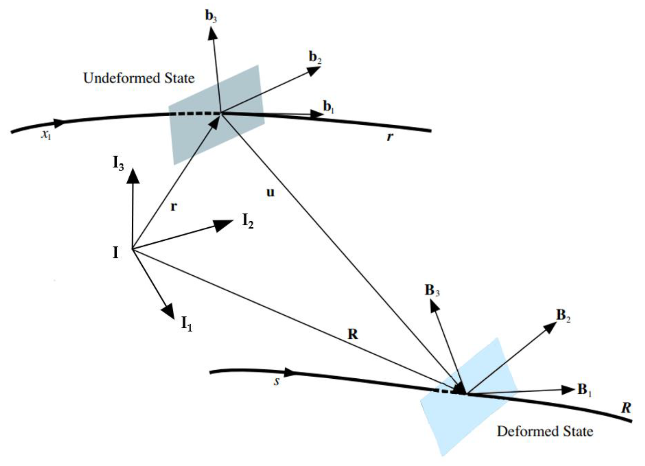
2. Fully Intrinsic Beam Equations of Geometrically Exact Beam

Figure 1 describes the geometric relationships of beams with initial bending and torsion before and after deformation, which was used by Hodges in 1990 [4]. $I$ Is the inertial coordinate system. $b_i(i = 1 ~ 3)$ is the basis vector of the undeformed reference coordinate system, and the origin is on the reference axis. $b_1$ is always tangent to the beam reference axis $x_1$, while $b_2$ and $b_3$ are always in the two-dimensional section of the beam, tangent to the reference axis of the beam. $B_i(i = 1 ~ 3)$ is the basis vector of the deformed reference coordinate system. Generally, the two-dimensional section of the beam will undergo shear deformation, so $B_1$ is not necessarily still parallel to the reference axis $s$ of the beam. $B_2$ and $B_3$ are used to represent the translation and rotation of the two-dimensional beam profile in the coordinate system after deformation. The vector $r$ represents the initial displacement relative to the inertial coordinate system $\mathrm{I}$. After deformation, the displacement becomes a vector $\mathrm{R}$. Thus, the actual displacement change of the beam can be expressed as:

$$\mathrm{R} = r + u$$

(1)

Combining the weak form of Hamilton’s principle, the constitutive relation of beam and the kinematic equation, Hodges [1,6] deduced the fully intrinsic equations of beam by eliminating the displacement and angle variables through the generalized strain-displacement and generalized velocity-displacement relations. Therefore, only the intrinsic quantities are retained in the equations, and the compact and concise equations are obtained as the following:

$$\begin{array}{l}{F^{\prime }}_B + (\tilde{k} + \tilde{\kappa })F_B + f_B = {\dot{P}}_B + {\tilde{\mathrm{\Omega }}}_B{P}_B\\ {M^{\prime }}_B + (\tilde{k} + \tilde{\kappa })M_B + ({\tilde{e}}_1 + \tilde{\gamma })F_B + m_B = {\dot{H}}_B + {\tilde{\mathrm{\Omega }}}_B{H}_B + {\tilde{V}}_B{P}_B\\ {V^{\prime }}_B + (\tilde{k} + \tilde{\kappa })V_B + ({\tilde{e}}_1 + \tilde{\gamma }){\mathrm{\Omega }}_B = {\dot{\gamma }}_B\\ {{\mathrm{\Omega }}^{\prime }}_B + (\tilde{k} + \tilde{\kappa }){\mathrm{\Omega }}_B = {\dot{\kappa }}_B\end{array}$$

(2)

The first two equations of Equation (2) are dynamic partial differential equations, while the last two are kinematic partial differential equations. Among them, ${( )}_B$ represents the observed quantity in the coordinate system after deformation. $( {)}^{\prime }$ represents the partial derivative with respect to the reference axis $x_1$ of the beam coordinate system. $(\dot{})$ is the partial derivative with respect to time. $F(x,t)$, $M(x,t)$, $V(x,t)$ and $\mathrm{\Omega }(x,t)$ are respectively the force, moment, linear velocity and angular velocity of the beam section. $\gamma (x,t)$, $\kappa (x,t)$, $P(x,t)$ and $H(x,t)$ respectively represents the generalized force strain, moment strain, linear momentum and angular momentum of the beam section. $f(x,t)$ and $m(x,t)$ respectively represents the distributed force and the distributed moment acting on the beam. $e_1 = {\left[\begin{array}{ccc}1& 0& 0\end{array}\right]}^T$. $k$ is the initial bending and torsion of the beam in the undeformed coordinate system, expressed as $k(x) = {\left[\begin{array}{ccc}{k}_1(x)& k_2(x)& k_3(x)\end{array}\right]}^T$. $\widetilde{( )}$ is the cross product operator that characterizes the extension of a column matrix to an antisymmetric matrix by dyadic operation [4], taking $k$ as an example:

$$\tilde{k} = \left[\begin{array}{ccc}& \hfill -k_3\hfill & \hfill k_2\hfill \\ \hfill k_3\hfill & & \hfill -k_1\hfill \\ \hfill -k_2\hfill & \hfill k_1\hfill & \end{array}\right]$$

(3)

Based on the hypothesis of small strain, the constitutive relation of beams is introduced by Hodges in [6]:

$$\left\{\begin{array}{c}\gamma \\ \kappa \end{array}\right\} = \left[\begin{array}{cc}R& S\\ S^T& \mathrm{T}\end{array}\right]\left\{\begin{array}{c}F\\ M\end{array}\right\}$$

(4)

Equation (4) is used to eliminate $\gamma$ and $\kappa$ from Equation (2) to retain the intrinsic variable $F$ and $M$. $R(x)$, $\mathrm{T}(x)$, $S(x)$ are the $3 \times 3$ matrix forms of the cross-sectional flexibilities of the beam, which can be calculated by finite element software such as VABS [32,33]. For a prismatic and isotropic beam, these flexibility matrices can be expressed as [1]:

$$R(x) = \left[\begin{array}{ccc}1/EA& 0& 0\\ 0& 1/G{K}_2& 0\\ 0& 0& 1/G{K}_3\end{array}\right] , \mathrm{T}(x) = \left[\begin{array}{ccc}1/GJ& 0& 0\\ 0& 1/E{I}_2& 0\\ 0& 0& 1/E{I}_3\end{array}\right] , \mathrm{S}(x) = \left[\begin{array}{ccc}0& 0& 0\\ 0& 0& 0\\ 0& 0& 0\end{array}\right]$$

(5)

Here, $EA$ and $G{K}_i(i = 2 ~ 3)$ are respectively the tensile and shear stiffness of the beam section, while $GJ$ and $E{I}_i(i = 2 ~ 3)$ respectively represent the torsional and bending stiffness of the beam section.

The generalized velocity-momentum equation of the beam is obtained from the density per unit length $\mu (x)$, section centroid bias $\overline{\xi }(x)$ and inertia matrix $I(x)$. The profile inertia coefficient matrix is represented by symbols $G$, $K$ and $I$:

$$\left\{\begin{array}{c}P\\ H\end{array}\right\} = \left[\begin{array}{cc}\mu \mathrm{\Delta }& -\mu \tilde{\overline{\xi }}\\ \mu \tilde{\overline{\xi }}& I\end{array}\right]\left\{\begin{array}{c}V\\ \mathrm{\Omega }\end{array}\right\} = \left[\begin{array}{cc}G& K\\ K^T& I\end{array}\right]\left\{\begin{array}{c}V\\ \mathrm{\Omega }\end{array}\right\}$$

(6)

In the above, $\mu$ is the mass per unit length, $\mathrm{\Delta }$ is the identity matrix of $3 \times 3$. $\overline{\xi }(x)$ is the offset of the centroid of the beam profile with respect to the reference axis of the beam, and ${\overline{x}}_2$, ${\overline{x}}_3$ are offsets in $b_2$, $b_3$, respectively. $I(x)$ is made up of mass moments of inertia $i_2$, $i_3$:

$$\overline{\xi }(x) = {\left[\begin{array}{ccc}0& {\overline{x}}_2& {\overline{x}}_3\end{array}\right]}_B^T, I = \left[\begin{array}{ccc}{i}_2 + i_3& & \\ & i_2& \\ & & i_3\end{array}\right]$$

(7)

Equation (6) is used to eliminate $P$ and $H$ from Equation (2) to preserve intrinsic variables $V$ and $\mathrm{\Omega }$. Therefore, Equations (2), (4) and (6) form a complete set of first-order partial equations about time and space.

3. Space-Time Finite Element Method of Fully Intrinsic Equations

3.1. Continuous Energy Weighting Method

It is assumed that beams are discretized into $n$ segments in the spatial direction $L$ and $m$ segments in the temporal direction $T$ to form a $n \times m$ space-time global grid, as shown in Figure 2, where the unit segment length of each space-time element $E_{ij}(i = 1 ~ n,j = 1 ~ m)$ in the spatial direction is denoted by $L^i$, and the unit segment length in the time direction is denoted by $T^j$. The intrinsic variables in the spatio-temporal unit are: $F(x^i,t^j)$, $M(x^i,t^j)$, $V(x^i,t^j)$ and $\mathrm{\Omega }(x^i,t^j)$, which can be simplified as $F^{ij}$, $M^{ij}$, $V^{ij}$, and ${\mathrm{\Omega }}^{ij}$.

Different from the conventional spatial finite element method, the space-time finite element method has an additional time dimension, so it needs to establish the continuity equations in both the space and time domain. According to the difference of space-derivative parameters and time-derivative parameters of the full intrinsic equations, the space and time continuity conditions are slightly different. On the spatial scale, consider $F$, $M$, $V$ and $\mathrm{\Omega }$ continuous:

$$\begin{array}{l}{F}^{i,j}(L^i,t^j) = F^{i + 1,j}(0,t^j),M^{i,j}(L^i,t^j) = M^{i + 1,j}(0,t^j)\\ V^{i,j}(L^i,t^j) = V^{i + 1,j}(0,t^j),{\mathrm{\Omega }}^{i,j}(L^i,t^j) = {\mathrm{\Omega }}^{i + 1,j}(0,t^j)\end{array}$$

(8)

Here, 0 represents the spatial start position and $L^i$ represents the spatial end position of the space-time element. On the time scale, consider $\gamma$, $\kappa$, $P$, and $H$ continuous:

$$\begin{array}{l}{\gamma }^{i,j}(x^i,T^j) = {\gamma }^{i,j + 1}(x^i,0),{\kappa }^{i,j}(x^i,T^j) = {\kappa }^{i,j + 1}(x^i,0)\\ P^{i,j}(x^i,T^j) = P^{i,j + 1}(x^i,0),H^{i,j}(x^i,T^j) = H^{i,j + 1}(x^i,0)\end{array}$$

(9)

Here, 0 represents the beginning time and $T^j$ represents the end time of the space-time element.

Dealing with space-time boundary conditions is the special case of space-time element continuity. Considering the introduction of intrinsic dynamic boundary conditions in space direction and steady-state response period conditions in the time direction:

$$\begin{array}{l}{F}^{n,j}(L^n,t^j) = F_L,M^{n,j}(L^n,t^j) = M_L\\ V^{1,j}(0,t^j) = V_0,{\mathrm{\Omega }}^{1,j}(0,t^j) = {\mathrm{\Omega }}_0\end{array}$$

(10)

$$\begin{array}{l}{\gamma }^{i,m}(x^i,T^m) = {\gamma }^{i,1}(x^i,0),{\kappa }^{i,m}(x^i,T^m) = {\kappa }^{i,1}(x^i,0)\\ P^{i,m}(x^i,T^m) = P^{i,1}(x^i,0),H^{i,m}(x^i,T^m) = H^{i,1}(x^i,0)\end{array}$$

(11)

The fully intrinsic Equation (2), space-time continuity conditions (8, 9) and space-time boundary conditions (10, 11) of geometrically exact beam can be assembled in the form of weighted residual:

$$\begin{array}{l}{\displaystyle {\int }_0^T{\displaystyle {\int }_0^L\left\{\begin{array}{l}{V}^T\left[\dot{P} + \tilde{\mathrm{\Omega }}P - F^{\prime } - (\tilde{k} + \tilde{\kappa })F - f\right]\\ + {\mathrm{\Omega }}^T\left[\dot{H} + \tilde{\mathrm{\Omega }}H + \tilde{V}P - M^{\prime } - (\tilde{k} + \tilde{\kappa })M - ({\tilde{e}}_1 + \tilde{\gamma })F - m\right]\\ + F^T\left[\dot{\gamma } - V^{\prime } - (\tilde{k} + \tilde{\kappa })V - ({\tilde{e}}_1 + \tilde{\gamma })\mathrm{\Omega }\right]\\ + M^T\left[\dot{\kappa } - {\mathrm{\Omega }}^{\prime } - (\tilde{k} + \tilde{\kappa })\mathrm{\Omega }\right]\end{array}\right\}dxdt}}\\ + {\displaystyle {\int }_0^T\left\{\begin{array}{l}{V}^T(L,t)\left[F(L,t) - F(0,t)\right] + {\mathrm{\Omega }}^T(L,t)\left[M(L,t) - M(0,t)\right]\\ + F^T(0,t)\left[V(L,t) - V(0,t)\right] + M^T(0,t)\left[\mathrm{\Omega }(L,t) - \mathrm{\Omega }(0,t)\right]\end{array}\right\}dt}\\ + {\displaystyle {\int }_0^L\left\{\begin{array}{l}{V}^T(x,T)\left[P(x,T) - P(x,0)\right] + {\mathrm{\Omega }}^T(x,T)\left[H(x,T) - H(x,0)\right]\\ + F^T(x,T)\left[\gamma (x,T) - \gamma (x,0)\right] + M^T(x,T)\left[\kappa (x,T) - \kappa (x,0)\right]\end{array}\right\}dx}\\ + {\displaystyle {\int }_0^T\left\{\begin{array}{l}{V}^T(L,t)\left[F(L,t) - F^L\right] + {\mathrm{\Omega }}^T(L,t)\left[M(L,t) - M^L\right]\\ + F^T(0,t)\left[V^0 - V(0,t)\right] + M^T(0,t)\left[{\mathrm{\Omega }}^0 - \mathrm{\Omega }(0,t)\right]\end{array}\right\}dt}\\ + {\displaystyle {\int }_0^L\left\{\begin{array}{l}{V}^T(L,0)\left[P(x,T) - P(x,0)\right] + {\mathrm{\Omega }}^T(L,0)\left[H(x,T) - H(x,0)\right]\\ + F^T(L,0)\left[\gamma (x,T) - \gamma (x,0)\right] + M^T(L,0)\left[\kappa (x,T) - \kappa (x,0)\right]\end{array}\right\}dx} = 0\end{array}$$

(12)

Among them, the first part is the expression of the weighted residual of the fully intrinsic equations. The second and third parts are the continuity conditions in space and time directions, respectively. The fourth and fifth parts are the space-boundary conditions and time-periodic conditions, respectively.

3.2. Legendre Polynomial Interpolation

Legendre interpolation polynomials are common test functions for finite element discretization, which satisfy the orthogonal relation as follows:

$${\displaystyle {\int }_0^1{p}^i(\overline{x})p^j(\overline{x})}d\overline{x} = \frac{{\delta }_{ij}}{2i + 1}$$

(13)

where, $\overline{x}$ represents the normalized variable whose domain is [0, 1], and the polynomials of each order are:

$$p^0\left(\overline{x}\right) = 1, p^1\left(\overline{x}\right) = 2\overline{x} - 1, p^{i + 1}\left(\overline{x}\right) = \frac{(2i + 1)(2\overline{x} - 1)p^i(\overline{x}) - i{p}^{i - 1}(\overline{x})}{i + 1}$$

(14)

In this paper, the linear Legendre interpolation polynomial is used as an example to derive the space-time finite element discrete equations of linear scheme. Take $N$ to represent the normalized dimension, use $x$ as the actual physical coordinate, then the first two-order Legendre interpolation polynomials are:

$$p^0\left(x\right) = 1, p^1\left(x\right) = 2\frac{x}{N} - 1$$

(15)

Since the two dimensions of time and space are independent, the components of the state parameters related to space and time can be divided into the form of the product of the two kinds of polynomials:

$$\begin{array}{l}{F}^{i,j}(x^i,t^j) = {\displaystyle \sum _{k = 0}^1{\displaystyle \sum _{l = 0}^1{p}^k\left({\overline{x}}^i\right)p^l\left({\overline{t}}^j\right)}}{f}^{ij,kl},M^{i,j}(x^i,t^j) = {\displaystyle \sum _{k = 0}^1{\displaystyle \sum _{l = 0}^1{p}^k\left({\overline{x}}^i\right)p^l\left({\overline{t}}^j\right)}}{m}^{ij,kl}\\ V^{i,j}(x^i,t^j) = {\displaystyle \sum _{k = 0}^1{\displaystyle \sum _{l = 0}^1{p}^k\left({\overline{x}}^i\right)p^l\left({\overline{t}}^j\right)}}{v}^{ij,kl},{\mathrm{\Omega }}^{i,j}(x^i,t^j) = {\displaystyle \sum _{k = 0}^1{\displaystyle \sum _{l = 0}^1{p}^k\left({\overline{x}}^i\right)p^l\left({\overline{t}}^j\right)}}{\omega }^{ij,kl}\end{array}$$

(16)

where, $f^{ij,kl}$, $m^{ij,kl}$, $v^{ij,kl}$ and ${\omega }^{ij,kl}$ are column vectors of unknown quantities in the equations, representing the weight coefficients of the $k(k = 0,1)$-th-order space scheme and the $l(l = 0,1)$-th order time scheme of the $(i,j)$-th space-time unit. The number of unknown variables of a space-time unit is $(12 \times 2 \times 2)$. The spatial and temporal derivatives of the intrinsic quantities can be expressed as the spatial and temporal derivatives of the interpolation polynomial, respectively. That is, the derivative with $\overline{x}$ respect to $p^k\left({\overline{x}}^i\right)$ and the derivative with $\overline{t}$ respect to $p^l\left({\overline{t}}^j\right)$:

$$\begin{array}{l}{F^{\prime }}^{i,j}(x^i,t^j)={\displaystyle \sum _{k = 0}^1{\displaystyle \sum _{l = 0}^1{p^{\prime }}^k\left({\overline{x}}^i\right)p^l\left({\overline{t}}^j\right)}}{f}^{ij,kl},{\dot{F}}^{i,j}(x^i,t^j)={\displaystyle \sum _{k = 0}^1{\displaystyle \sum _{l = 0}^1{p}^k\left({\overline{x}}^i\right){\dot{p}}^l\left({\overline{t}}^j\right)}}{f}^{ij,kl}\\ {M^{\prime }}^{i,j}(x^i,t^j) = {\displaystyle \sum _{k = 0}^1{\displaystyle \sum _{l = 0}^1{p^{\prime }}^k\left({\overline{x}}^i\right)p^l\left({\overline{t}}^j\right)}}{m}^{ij,kl},{\dot{M}}^{i,j}(x^i,t^j) = {\displaystyle \sum _{k = 0}^1{\displaystyle \sum _{l = 0}^1{p}^k\left({\overline{x}}^i\right){\dot{p}}^l\left({\overline{t}}^j\right)}}{m}^{ij,kl}\\ {V^{\prime }}^{i,j}(x^i,t^j) = {\displaystyle \sum _{k = 0}^1{\displaystyle \sum _{l = 0}^1{p^{\prime }}^k\left({\overline{x}}^i\right)p^l\left({\overline{t}}^j\right)}}{v}^{ij,kl},{\dot{V}}^{i,j}(x^i,t^j) = {\displaystyle \sum _{k = 0}^1{\displaystyle \sum _{l = 0}^1{p}^k\left({\overline{x}}^i\right){\dot{p}}^l\left({\overline{t}}^j\right)}}{v}^{ij,kl}\\ {{\mathrm{\Omega }}^{\prime }}^{i,j}(x^i,t^j) = {\displaystyle \sum _{k = 0}^1{\displaystyle \sum _{l = 0}^1{p^{\prime }}^k\left({\overline{x}}^i\right)p^l\left({\overline{t}}^j\right)}}{\omega }^{ij,kl},{\dot{\mathrm{\Omega }}}^{i,j}(x^i,t^j) = {\displaystyle \sum _{k = 0}^1{\displaystyle \sum _{l = 0}^1{p}^k\left({\overline{x}}^i\right){\dot{p}}^l\left({\overline{t}}^j\right)}}{\omega }^{ij,kl}\end{array}$$

(17)

Therefore, taking ansatzes (15), (16) and (17) into Equation (12), the Galerkin approximation of the original equation can be obtained. The specific integral equations are given in Appendix A.

3.3. Constant Cross-Section, Curvature

To facilitate the application of the present method, we assume that the two-dimensional profile characteristics ($R$, $T$, $S$, $G$, $I$, $K$) and the curvature $k$ remain constant in the space-time unit. With this assumption, they can be moved out from the integral expressions:

$$\begin{array}{l}{A}_x^{\alpha k}{L}^i{B}_t^{\beta l}\left(G^{ij}{v}^{ij,kl} + K^{ij}{\omega }^{ij,kl}\right) + C_x^{\alpha kp}{L}^i{C}_t^{\beta lq}{T}^j\widetilde{{\omega }^{ij,pq}}\left(G^{ij}{v}^{ij,kl} + K^{ij}{\omega }^{ij,kl}\right)\\ - B_x^{\alpha k}{A}_t^{\beta l}{T}^j{f}^{ij,kl} - A_x^{\alpha k}{L}^i{A}_t^{\beta l}{T}^j{\tilde{k}}^{ij}{f}^{ij,kl} - C_x^{\alpha kp}{L}^i{C}_t^{\beta lq}{T}^j\left(\widetilde{S^{{}_{ij}^T}{f}^{ij,pq}} + \widetilde{T^{ij}{m}^{ij,pq}}\right)f^{ij,kl}\\ - D_x^{\alpha }{L}^i{D}_t^{\beta }{T}^j{\mathrm{f}}^{ij}\\ + \left[p_x^{\alpha }\left(1\right)p_x^k\left(1\right)A_t^{\beta l}{T}^j{f}^{ij,kl} - p_x^{\alpha }\left(1\right)p_x^k\left(0\right)A_t^{\beta l}{T}^j{f}^{(i + 1)j,kl}\right]\\ + \left[\begin{array}{l}{A}_x^{\alpha k}{L}^i{p}_t^{\beta }(1)p_t{}^l\left(1\right)G^{ij}{v}^{ij,kl} - A_x^{\alpha k}{L}^i{p}_t^{\beta }(1)p_t{}^l\left(0\right)G^{i(j + 1)}{v}^{i(j + 1),kl}\\ + A_x^{\alpha k}{L}^i{p}_t^{\beta }(1)p_t{}^l\left(1\right)K^{ij}{\omega }^{ij,kl} - A_x^{\alpha k}{L}^i{p}_t^{\beta }(1)p_t{}^l\left(0\right)K^{i(j + 1)}{\omega }^{i(j + 1),kl}\end{array}\right] = 0\end{array}$$

(18)

$$\begin{array}{l}{A}_x^{\alpha k}{L}^i{B}_t^{\beta l}\left(K^{{}_{ij}^T}{v}^{ij,kl} + I^{ij}{\omega }^{ij,kl}\right) + C_x^{\alpha kp}{L}^i{C}_t^{\beta lq}{T}^j\widetilde{{\omega }^{ij,pq}}\left(K^{{}_{ij}^T}{v}^{ij,kl} + I^{ij}{\omega }^{ij,kl}\right)\\ + C_x^{\alpha kp}{L}^i{C}_t^{\beta lq}{T}^j\widetilde{v^{ij,pq}}\left(G^{ij}{v}^{ij,kl} + K^{ij}{\omega }^{ij,kl}\right) - B_x^{\alpha k}{A}_t^{\beta l}{T}^j{m}^{ij,kl}\\ - A_x^{\alpha k}{L}^i{A}_t^{\beta l}{T}^j{\tilde{k}}^{ij}{m}^{ij,kl} - C_x^{\alpha kp}{L}^i{C}_t^{\beta lq}{T}^j\left(\widetilde{S^{{}_{ij}^T}{f}^{ij,pq}} + \widetilde{T^{ij}{m}^{ij,pq}}\right)m^{ij,kl}\\ - A_x^{\alpha k}{L}^i{A}_t^{\beta l}{T}^j{\tilde{e}}_1{f}^{ij,kl} - C_x^{\alpha kp}{L}^i{C}_t^{\beta lq}{T}^j\left(\widetilde{R^{ij}{f}^{ij,pq}} + \widetilde{S^{ij}{m}^{ij,pq}}\right)f^{ij,kl}\\ - D_x^{\alpha }{L}^i{D}_t^{\beta }{T}^j{\mathrm{m}}^{ij}\\ + \left[p_x^{\alpha }\left(1\right)p_x^k\left(1\right)A_t^{\beta l}{T}^j{m}^{ij,kl} - p_x^{\alpha }\left(1\right)p_x^k\left(0\right)A_t^{\beta l}{T}^j{m}^{(i + 1)j,kl}\right]\\ + \left[\begin{array}{l}{A}_x^{\alpha k}{L}^i{p}_t^{\beta }(1)p_t{}^l\left(1\right)K^{{}_{ij}^T}{v}^{ij,kl} - A_x^{\alpha k}{L}^i{p}_t^{\beta }(1)p_t{}^l\left(0\right)K^{{}_{i(j + 1)}^T}{v}^{i(j + 1),kl}\\ + A_x^{\alpha k}{L}^i{p}_t^{\beta }(1)p_t{}^l\left(1\right)I^{ij}{\omega }^{ij,kl} - A_x^{\alpha k}{L}^i{p}_t^{\beta }(1)p_t{}^l\left(0\right)I^{i(j + 1)}{\omega }^{i(j + 1),kl}\end{array}\right] = 0\end{array}$$

(19)

$$\begin{array}{l}{A}_x^{\alpha k}{L}^i{B}_t^{\beta l}\left(R^{ij}{f}^{ij,kl} + S^{ij}{m}^{ij,kl}\right) - B_x^{\alpha k}{A}_t^{\beta l}{T}^j{v}^{ij,kl}\\ - A_x^{\alpha k}{L}^i{A}_t^{\beta l}{T}^j{\tilde{k}}^{ij}{v}^{ij,kl} - C_x^{\alpha kp}{L}^i{C}_t^{\beta lq}{T}^j\left(\widetilde{S^{{}_{ij}^T}{f}^{ij,pq}} + \widetilde{T^{ij}{m}^{ij,pq}}\right)v^{ij,kl}\\ - A_x^{\alpha k}{L}^i{A}_t^{\beta l}{T}^j{\tilde{e}}_1{\omega }^{ij,kl} - C_x^{\alpha kp}{L}^i{C}_t^{\beta lq}{T}^j\left(\widetilde{R^{ij}{f}^{ij,pq}} + \widetilde{S^{ij}{m}^{ij,pq}}\right){\omega }^{ij,kl}\\ + \left[p_x^{\alpha }\left(1\right)p_x^k\left(1\right)A_t^{\beta l}{T}^j{v}^{(i - 1)j,kl} - p_x^{\alpha }\left(1\right)p_x^k\left(0\right)A_t^{\beta l}{T}^j{v}^{ij,kl}\right]\\ + \left[\begin{array}{l}{A}_x^{\alpha k}{L}^i{p}_t^{\beta }(1)p_t{}^l\left(1\right)R^{ij}{f}^{ij,kl} - A_x^{\alpha k}{L}^i{p}_t^{\beta }(1)p_t{}^l\left(0\right)R^{i(j + 1)}{f}^{i(j + 1),kl}\\ + A_x^{\alpha k}{L}^i{p}_t^{\beta }(1)p_t{}^l\left(1\right)S^{ij}{m}^{ij,kl} - A_x^{\alpha k}{L}^i{p}_t^{\beta }(1)p_t{}^l\left(0\right)S^{i(j + 1)}{m}^{i(j + 1),kl}\end{array}\right] = 0\end{array}$$

(20)

$$\begin{array}{l}{A}_x^{\alpha k}{L}^i{B}_t^{\beta l}\left(S^{{}_{ij}^T}{f}^{ij,kl} + T^{ij}{m}^{ij,kl}\right) - B_x^{\alpha k}{A}_t^{\beta l}{T}^j{\omega }^{ij,kl}\\ - A_x^{\alpha k}{L}^i{A}_t^{\beta l}{T}^j{\tilde{k}}^{ij}{\omega }^{ij,kl} - C_x^{\alpha kp}{L}^i{C}_t^{\beta lq}{T}^j\left(\widetilde{S^{{}_{ij}^T}{f}^{ij,pq}} + \widetilde{T^{ij}{m}^{ij,pq}}\right){\omega }^{ij,kl}\\ + \left[p_x^{\alpha }\left(1\right)p_x^k\left(1\right)A_t^{\beta l}{T}^j{\omega }^{(i - 1)j,kl} - p_x^{\alpha }\left(1\right)p_x^k\left(0\right)A_t^{\beta l}{T}^j{\omega }^{ij,kl}\right]\\ + \left[\begin{array}{l}{A}_x^{\alpha k}{L}^i{p}_t^{\beta }(1)p_t{}^l\left(1\right)S^{{}_{ij}^T}{f}^{ij,kl} - A_x^{\alpha k}{L}^i{p}_t^{\beta }(1)p_t{}^l\left(0\right)S^{{}_{i(j + 1)}^T}{f}^{i(j + 1),kl}\\ + A_x^{\alpha k}{L}^i{p}_t^{\beta }(1)p_t{}^l\left(1\right)T^{ij}{m}^{ij,kl} - A_x^{\alpha k}{L}^i{p}_t^{\beta }(1)p_t{}^l\left(0\right)T^{i(j + 1)}{m}^{i(j + 1),kl}\end{array}\right] = 0\end{array}$$

(21)

where the coefficients $A_x^{\alpha k}$, $A_t^{\beta l}$, $B_x^{\alpha k}$, $B_t^{\beta l}$, $C_x^{\alpha kp}$, $C_t^{\beta lq}$, $D_x^{\alpha }$, and $D_t^{\beta }$ are dimensionless integral operators, respectively:

$$\begin{array}{l}{A}_x^{\alpha k} = {\displaystyle {\int }_0^1{p}^{\alpha }\left(\overline{x}\right)}{p}^k\left(\overline{x}\right)d\overline{x},A_t^{\beta l} = {\displaystyle {\int }_0^1{p}^{\beta }\left(\overline{t}\right)}{p}^l\left(\overline{t}\right)d\overline{t}\\ B_x^{\alpha k} = {\displaystyle {\int }_0^1{p}^{\alpha }\left(\overline{x}\right)}{p^{\prime }}^k\left(\overline{x}\right)d\overline{x},B_t^{\beta l} = {\displaystyle {\int }_0^1{p}^{\beta }\left(\overline{t}\right)}{\dot{p}}^l\left(\overline{t}\right)d\overline{t}\\ C_x^{\alpha kp} = {\displaystyle {\int }_0^1{p}^{\alpha }\left(\overline{x}\right)}{p}^k\left(\overline{x}\right)p^p\left(\overline{x}\right)d\overline{x},C_t^{\beta lq} = {\displaystyle {\int }_0^1{p}^{\beta }\left(\overline{t}\right)}{p}^l\left(\overline{t}\right)p^q\left(\overline{t}\right)d\overline{t}\\ D_x^{\alpha } = {\displaystyle {\int }_0^1{p}^{\alpha }\left(\overline{x}\right)}d\overline{x},D_t^{\beta } = {\displaystyle {\int }_0^1{p}^{\beta }\left(\overline{t}\right)}d\overline{t}\end{array}$$

(22)

Therefore, the above equations can be succinctly expressed as:

$$B_{ele}\cdot q_{ele} + {\mathit{Hs}}_{ele}\cdot {\mathit{qs}}_{ele} + {\mathit{Ht}}_{ele}\cdot {\mathit{qt}}_{ele} + C_{ele}(q_{ele})\cdot q_{ele} + D_{ele} = 0$$

(23)

Among these, $B_{ele}$ is the linear array of the space-time element, ${\mathit{Hs}}_{ele}$ and ${\mathit{Ht}}_{ele}$ represent the connection matrix of the space-time element in space and time, respectively. $C_{ele}$ characterizes the degree of nonlinearity of the element, and $D_{ele}$ is the constant vector. Besides, ${\mathit{qs}}_{ele}$ contains degrees of freedom of the preceding space-time unit $(i - 1,j)$, the current space-time unit, and the next space-time unit $(i + 1,j)$. ${\mathit{qt}}_{ele}$ contains degrees of freedom of the preceding space-time unit $(i,j - 1)$, the current space-time unit and the next space-time unit. $q_{ele}$ is the unknown quantity of the current space-time unit $(i,j)$, and its arrangement is as follows:

$$q_{ele}(x^i,t^j) = {\left\{\begin{array}{c}\begin{array}{cccccccc}{v}^{00}& v^{01}& v^{10}& v^{11}& w^{00}& w^{01}& w^{10}& w^{11}\end{array}\\ \dots \begin{array}{cccccccc}{f}^{00}& f^{01}& f^{10}& f^{11}& m^{00}& m^{01}& m^{10}& m^{11}\end{array}\end{array}\right\}}^T$$

(24)

3.4. Matrix Assembly

Due to the two-dimensional property of simultaneous discrete space-time, two directions of space and time should be considered in the matrix assembly. This paper adopts the assembly schedule of first space and then time. For a beam divided into $n$ spatial structural units, the space-time array derived above is assembled successively in the order of structural units, as shown in expressions (25) and (26). $B^j$ is the linear structure matrix of the space element group under the first time node, the main diagonal element is the linear matrix of each space element ($1,2,\cdots ,n$) under the $j$-th time node, and the off-diagonal element represents the connection matrix of adjacent space elements, shown as Appendix B. $C^j$ and $D^j$ correspond to nonlinear matrix and constant vector, respectively.

$$B^j = \left[\begin{array}{cccccc}{B}_{ele}^1& {\mathit{Hs}}_{ele2}& & & & \\ {\mathit{Hs}}_{ele1}& B_{ele}^2& {\mathit{Hs}}_{ele2}& & & \\ & {\mathit{Hs}}_{ele1}& B_{ele}^3& \ddots & & \\ & & {\mathit{Hs}}_{ele1}& \ddots & {\mathit{Hs}}_{ele2}& \\ & & & \ddots & B_{ele}^{n - 1}& {\mathit{Hs}}_{ele2}\\ & & & & {\mathit{Hs}}_{ele1}& B_{ele}^n\end{array}\right]$$

(25)

$$C^j = \left[\begin{array}{cccccc}{C}_{ele}^1& & & & & \\ & C_{ele}^2& & & & \\ & & C_{ele}^3& & & \\ & & & \ddots & & \\ & & & & C_{ele}^{n - 1}& \\ & & & & & C_{ele}^n\end{array}\right] , D^j = \left\{\begin{array}{c}{D}_{ele}^1\\ D_{ele}^2\\ D_{ele}^3\\ ⋮\\ D_{ele}^{n - 1}\\ D_{ele}^n\end{array}\right\}$$

(26)

In the time domain, $m$ time units are divided, and the operation is similar to that of space, which is gradually superimposed with the order of time units, as shown in expressions (27) and (28), where ${\mathit{Ht}}_{ele}$ is the connection array of adjacent time units, shown as Appendix C. It is worth noting that the upper right corner of expression (27) represents periodic boundary conditions.

$$B_{total} = \left[\begin{array}{ccccc}{B}^1& & & & {\mathit{Ht}}_{ele}\\ {\mathit{Ht}}_{ele}& B^2& & & \\ & {\mathit{Ht}}_{ele}& \ddots & & \\ & & \ddots & B^{m - 1}& \\ & & & {\mathit{Ht}}_{ele}& B^m\end{array}\right]$$

(27)

$$C_{total} = \left[\begin{array}{ccccc}{C}^1& & & & \\ & C^2& & & \\ & & \ddots & & \\ & & & C^{m - 1}& \\ & & & & C^m\end{array}\right] , D_{total} = \left\{\begin{array}{c}{D}^1\\ D^2\\ ⋮\\ D^{m - 1}\\ D^m\end{array}\right\}$$

(28)

Therefore, the full intrinsic equations of a geometrically accurate beam can be written in the following form after simultaneous discretization of space and time:

$$B_{total}{q}_{total} + C_{total}(q_{total})\cdot q_{total} + D_{total} = 0$$

(29)

Here, $B_{total}$ is the space-time discrete linear array, $C_{total}$ is the space-time discrete nonlinear array, $D_{total}$ is the constant vector, $q_{total}$ is all the unknowns in the space and time domain. It is obvious that this is a set of nonlinear algebraic equations, so nonlinear iteration is needed to solve them.

3.5. Post Process

Since the fully intrinsic equations do not contain the displacement and rotation variables, it is necessary to obtain the displacement variables through additional post process. Sotoudeh [11] et al., gave an expression for calculating the cosine matrix of displacement and direction at any point:

$$\begin{array}{l}\left\{\begin{array}{c}{r}_i^{\prime } = C^{ib}{e}_1\\ {(r_i + u_i)}^{\prime } = C^{iB}(e_1 + \gamma )\end{array}\right.\\ \left\{\begin{array}{c}{(C^{bi})}^{\prime } =-\tilde{k}{C}^{bi}\\ (C^{Bi}{)}^{\prime } =-(\tilde{k} + \tilde{\kappa })C^{Bi}\end{array}\right.\end{array}$$

(30)

3.6. Process of Simulation

In this paper, the organization process of the algorithm is summarized below, using the weighted margin method and the Galerkin integral, to solve the fully intrinsic equations of a geometrically exact beam in both time and space, as shown in Figure 3. It is mainly divided into three parts: energy consistent weighting, space-time element discretization and equations solving. The concrete steps are described as follows:

(1)

For a single space-time unit, consider the continuity of $F$, $M$, $V$, and $\mathrm{\Omega }$ in space. Meanwhile, consider the continuity of $\gamma$, $\kappa$, $P$ and $H$ in time. The unit needs special continuity operation at the space-time boundary conditions, see Formulas (8) and (10), and Formulas (9) and (11).

(2)

Combined with the constitutive relation, momentum-velocity relation and continuity condition, a set of energy balance equations in the form of a double integral of time and space is derived from the full intrinsic equations by using the weighted margin technique.

(3)

In the process of integral, the Legendre interpolation polynomial is used as a discrete function of intrinsic quantity. The specific expressions of linear matrix, nonlinear matrix, time-connected matrix, spatial connected matrix, and constant vector of single space-time element are derived based on the Galerkin approximation.

(4)

In the dimensionality of space and time, the coefficient matrix of a single space-time unit derived in the previous step can be assembled into a total coefficient matrix. Thus, the final discrete equations will be expressed as $B_{total}q + C_{total}(q)\cdot q + D_{total} = 0$.

(5)

For the derivation of nonlinear algebraic equations, solve equation of $B_{total}q + D_{total} = 0$ as the iteration start value. Then the Newton iteration method was used to get the convergent solution.

(6)

After obtaining the convergence solution, in addition to extracting the intrinsic quantity, the displacement response at any point can be obtained by applying its generalized strain through the post-processing process.

4. Numerical Results

In order to verify the applicability of the time-space discretization scheme derived in this paper for solving the fully intrinsic equations, three cases are considered. The first example analyzes the large deformation trajectories of the cantilever beam under different follower moments. The second example calculates the large deformation geometries of the cantilever beam under different following forces. The first two cases verify the effectiveness of space-time discrete format in dealing with static problems by calculating the following force and moment of cantilever beam. The last case considers the dynamic response of the rotating cantilever beam and compares it with other existing discrete schemes to verify the accuracy and efficiency.

4.1. Static Analysis and Modal Calculation of the Cantilever Beam

Consider applying a following moment to the tip of a cantilever beam to analyze the large deformation it experiences. Bending stiffness of cantilever beam $EI = 9000{ \mathrm{lb}\text{-}\mathrm{ft}}^2$, beam length $L = 20 \mathrm{ft}$. In [34], the analytical expression of the beam displacement was presented:

$$r_x = \rho \sin \frac{s}{\rho } , r_y = \rho (1 - \cos \frac{s}{\rho })$$

(31)

where, $r_x$ and $r_y$ is any point on the beam deformation curve. $\rho$ is the radius of curvature.

$\rho = EI/M_L = 18 \mathrm{ft}$, when the follower moment $M_L = 500 \mathrm{ft}\text{-}\mathrm{lb}$. When the moment is increased to $2500 \mathrm{ft}\text{-}\mathrm{lb}$, the radius of curvature becomes $3.6 \mathrm{ft}$. Different numbers of space-time elements are used to calculate the displacement of the beam at the tip, as shown in

Table 1. The results of tip displacement under various follower moments (unit: ft).

$M_L$	No. of Units	2	3	4	5	10	20
500 N.m	Exact	10.01401161
	STFEM	10.01401208	10.01401181	10.01401166	10.01401158	10.01401158	10.01401158
	Error	4.74 × 10−8	2.00 × 10−8	0.50 × 10−8	0.26 × 10−8	0.26 × 10−8	0.26 × 10−8
2500 N.m	Exact	0.91168936
	STFEM	0.91174717	0.91165092	0.91167167	0.91168341	0.91168634	0.91168896
	Error	6.34 × 10−5	4.22 × 10−5	1.94 × 10−5	0.65 × 10−5	0.33 × 10−5	4.39 × 10−7

. When the tip moment is $500 \mathrm{ft}\text{-}\mathrm{lb}$, even if two space-time elements are used for calculation, the relative error magnitude of displacement still reaches 4.74 × 10⁻⁸ The RCAS model in [34] uses 20 elements, and the error magnitude reaches 6.00 × 10⁻⁴. The accuracy of this method is still four orders of magnitude higher when using smaller computational cost. When the tip bending moment is $2500 \mathrm{ft}\text{-}\mathrm{lb}$, the accuracy of this method is lower than that of $500 \mathrm{ft}\text{-}\mathrm{lb}$. This is because the deformation of the beam is large and more time-space elements are needed for discretization. Nevertheless, the error magnitude of this method is still maintained at 1.00 × 10⁻⁵, which is better than 1.98 × 10⁻⁴ of RCAS. When the number of space-time elements is increased to 20, the error magnitude can be reduced to 4.39 × 10⁻⁷. Figure 4 shows the deformed configuration of the cantilever beam under various follower moments. It can be seen from the figure that the discrete solution calculated by this method is in good agreement with the analytical solution. When a periodic follower moment $2500\sin (t) \mathrm{ft}\text{-}\mathrm{lb}$ is applied to the tip, the large deformed configuration of the beam in the whole period is shown in Figure 5. The configuration is upswing-return-downswing-return, just like a person waving a rope up and down. The two blue dashed lines in the figure represent the trajectories of the node at 5 ft and 20 ft in the whole period.

Combined with Figure 6, it can be clearly seen that the closer the node is to the tip of the beam, the higher the position its movement can reach. At the same time, nodes can pass through this highest position more times throughout the period. This also means that the closer the node is to the tip, the more abundant the harmonic components of the node’s response are contained.

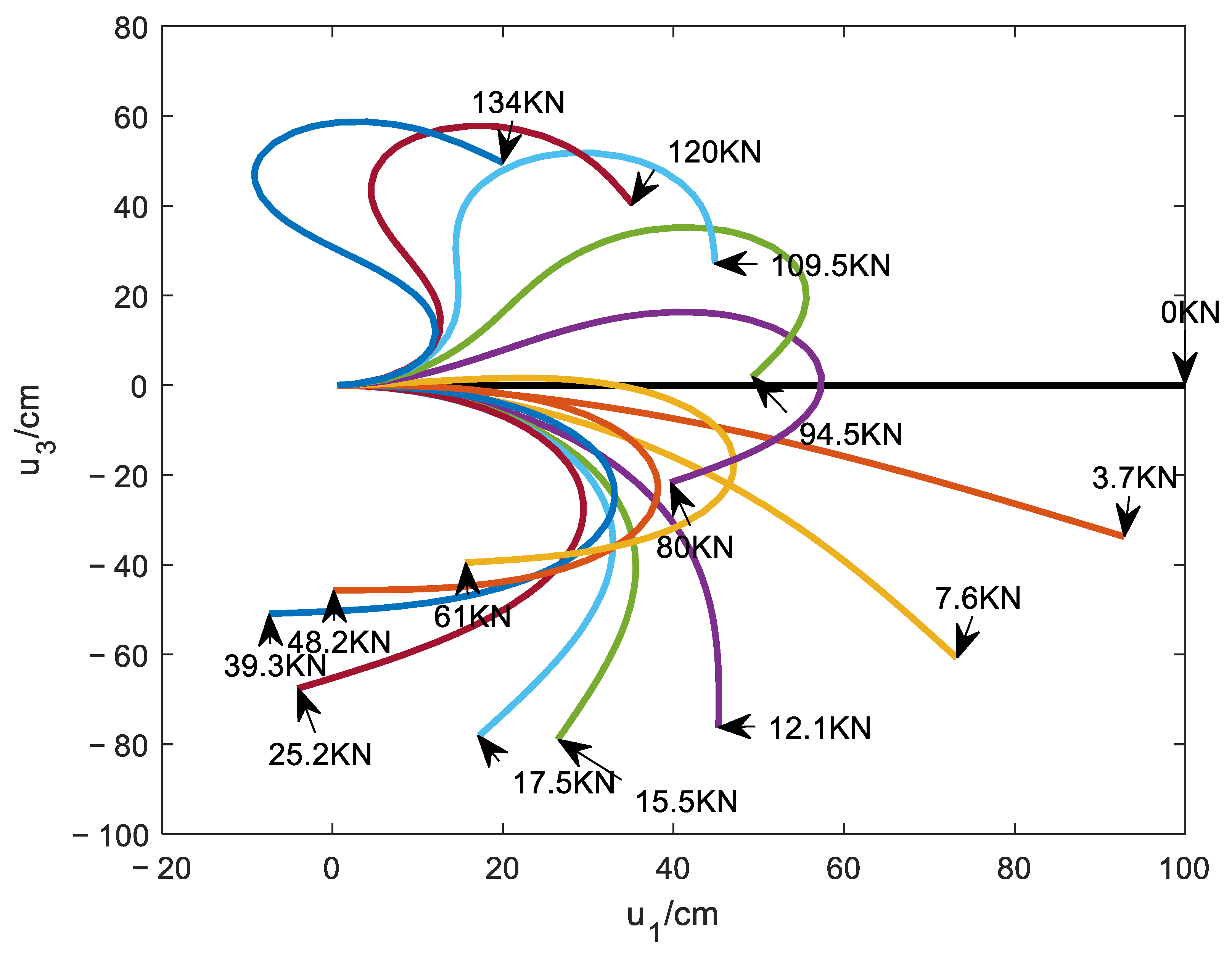
4.2. Cantilever Subjected to a Follower Force at the Tip

Consider applying a following force to the tip of the cantilever to analyze its deformed configuration. The length of the beam $L = 100\mathrm{cm}$, the moment of inertia $I_{22} = 1.666667{\mathrm{cm}}^4$, Young’s modulus $E = 2.1 \times {10}^7 \mathrm{N}/{\mathrm{cm}}^2$.

Figure 7 shows the load-displacement diagram at the free end, and the trajectory of the highly nonlinear deformation experienced by the beam can be obtained in Figure 8. It can be seen from Figure 7 that the calculation results of the present method are in good agreement with those calculated by Argyris in [35]. Except for the curve of $u_1$, when $F_L$ is around $\left[20,40\right]$ KN, the calculation results of this paper are quite different from those of the literature. Observing Figure 8 and Figure 6.4.3 in [35], it can be seen that when $F_L$ is 39.3 KN, $u_1$ is negative, and $-u_1/L$ in the corresponding Figure 7 must be greater than 1. Therefore, compared with the calculation results of the literature, the calculation results of this present method are more reasonable.

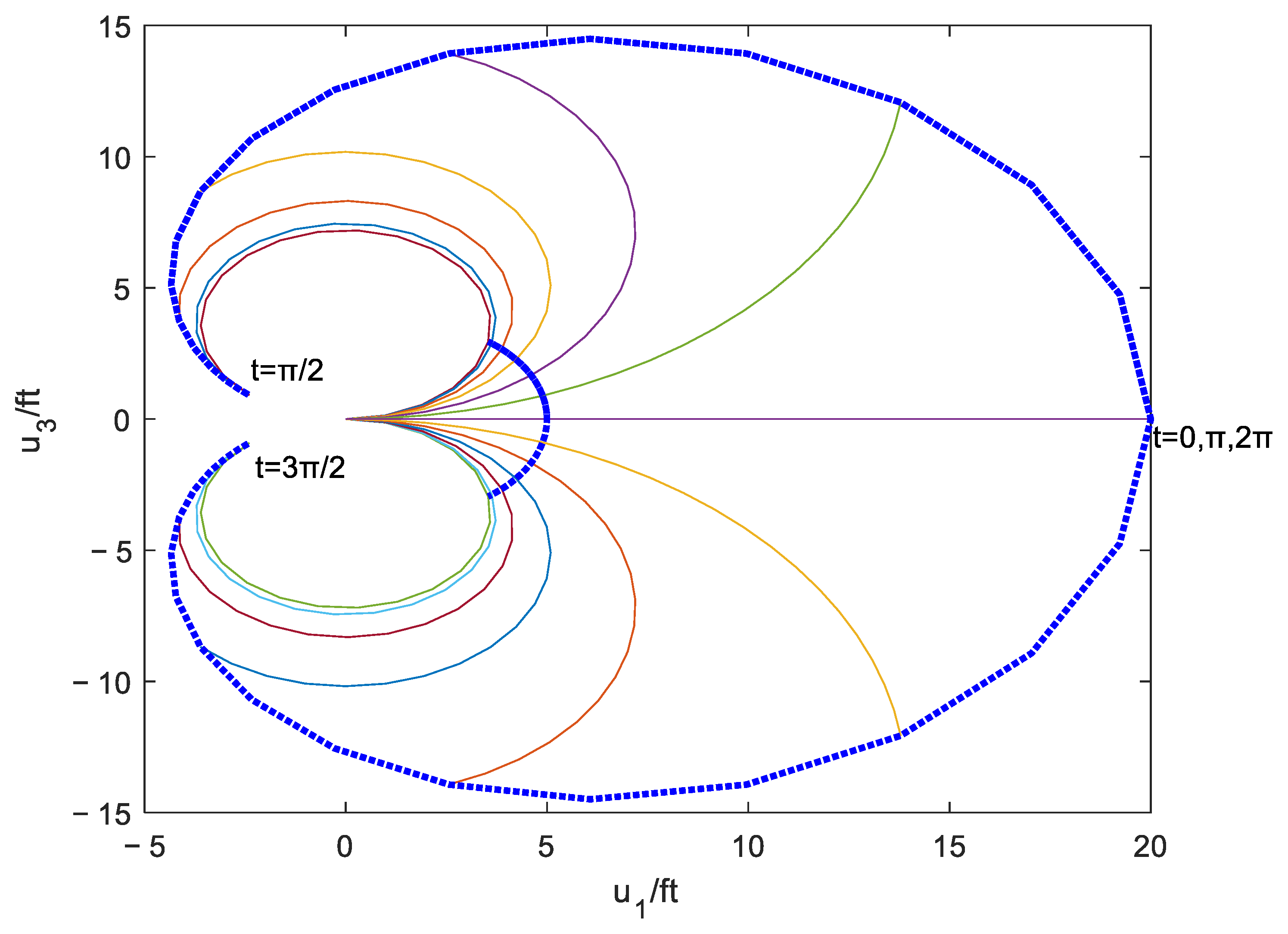
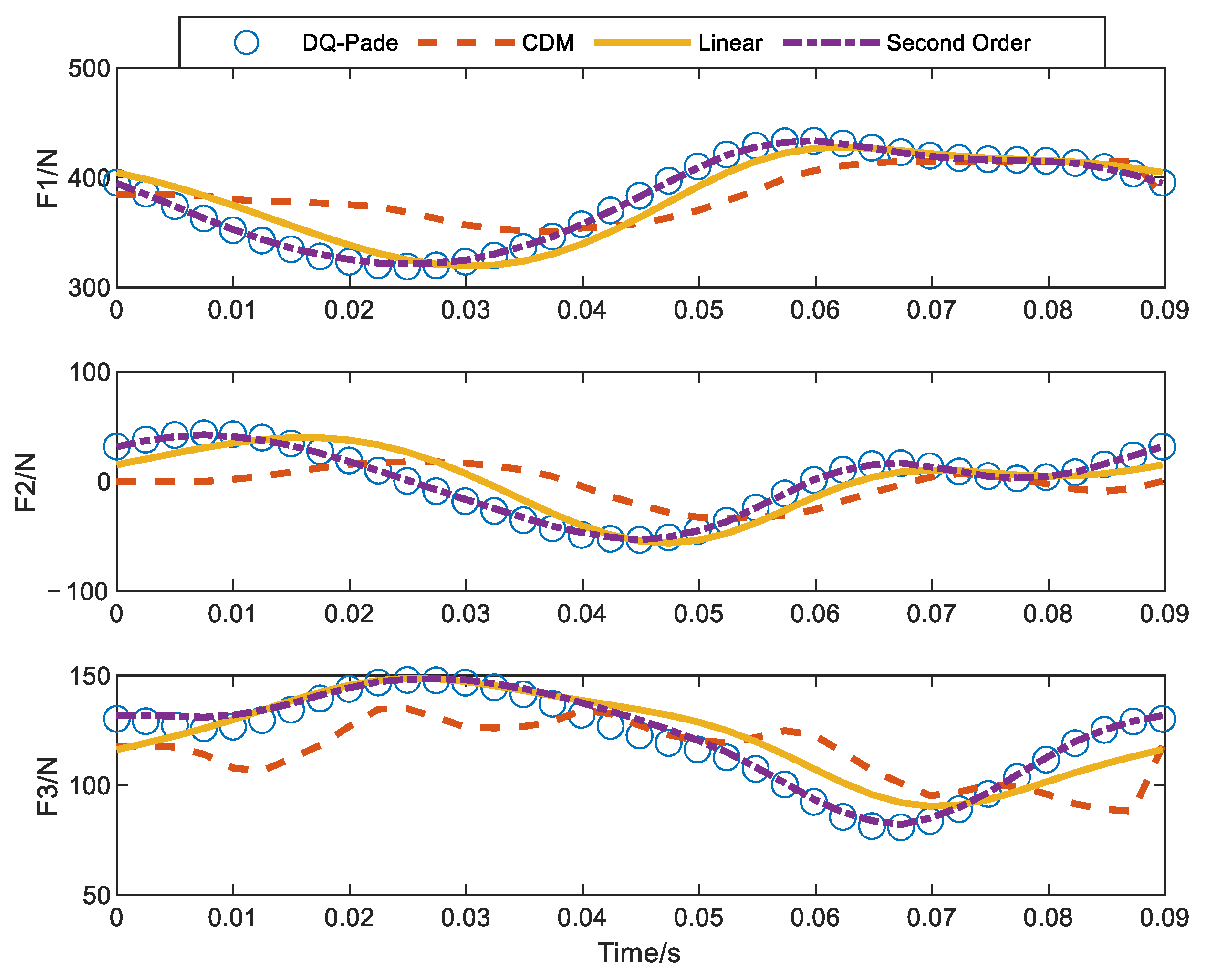
4.3. The Rotating Cantilever Subjected to a Periodic Follower Force at the Tip

The steady-state dynamic response calculation of a rotating cantilever beam is considered. The length of the beam $L = 1 \mathrm{m}$, the rotating speed $\mathrm{\Omega } = 70 \mathrm{r}\mathrm{a}\mathrm{d}/\mathrm{s}$. In [14], the researchers gave the material properties of the beam, as shown in

Table 2. Material properties of the beam.

Parameter	Value
Mass per unit length	$0.2 (\mathrm{kg}/\mathrm{m})$
Moment of inertia per unit length $I_{xx}$	${10}^{-4} (\mathrm{kg}\cdot \mathrm{m})$
Moment of inertia per unit length $I_{yy}$	${10}^{-6} (\mathrm{kg}\cdot \mathrm{m})$
Moment of inertia per unit length $I_{zz}$	${10}^{-4} (\mathrm{kg}\cdot \mathrm{m})$
Extensional rigidity $K_{11}$	${10}^6 \mathrm{N}$
Shear rigidity $K_{22}$	${10}^{20} \mathrm{N}$
Shear rigidity $K_{33}$	${10}^{20} \mathrm{N}$
Torsional rigidity $K_{44}$	$50 \mathrm{N}\cdot {\mathrm{m}}^2$
Bending rigidity $K_{55}$	$50 \mathrm{N}\cdot {\mathrm{m}}^2$
Bending rigidity (chordwise) $K_{66}$	$1000 \mathrm{N}\cdot {\mathrm{m}}^2$

.

A periodic follower force $F_3 = 150 + 10\sin (70t) + 5\sin (2\cdot 70t) + 2\sin (3\cdot 70t) \mathrm{N}$ is applied to the tip of the beam. A similar situation was calculated in [18] and the results were in good agreement with the multibody dynamics software Dymore and Euler method. Therefore, this paper uses the calculation results of its algorithm (DQ-Pade) as a comparison, which chooses 30 points in space and 72 points (M8/N9 scheme in [18]) in time direction. The central difference space-time element method (CDM) proposed by Hodges [4] is compared with the space-time finite element method derived in this paper. Furthermore, in order to test the characteristics of the proposed algorithm, the calculation results of the second-order space-time element are also given here.

In order to ensure the fairness of the comparison, the steady-state dynamic response of the rotating beam needs to be calculated under the same calculation cost. For the linear space-time element, 15 space-time elements are divided in space and 36 space-time elements are divided in time. For the second-order space-time element, it is necessary to divide 10 elements in the spatial direction and 24 elements in the time direction, so that the total number of discrete points in the time-space direction of the beam is $15 \times 36 \times (2*2) = 2160 = 10 \times 24 \times (3 \times 3)$. For CDM, the same space-time step as the linear space-time element is used to recursively solve both in time and space directions until convergence. Figure 9 and Figure 10 show the steady-state periodic curves of forces and moments at the root of the beam. Figure 11 and Figure 12 show the changing curves of section forces and moments along the spanwise direction of beam at $t = 0$. It can be seen from these figures that the second-order space-time element performs best under the same computational cost among the three algorithms, followed by the linear space-time element, and the CDM has a certain gap in accuracy with the first two. If we continue to subdivide the linear space-time finite element, we mainly consider the refinement in the time direction (the reason is that this is a periodic problem first, and then due to the centrifugal force of the rotating beam. In addition to the $\lambda = \raisebox{1ex}{$F$}\!\left/ \!\raisebox{-1ex}{$K_{55}$}\right. < 4$ in this example, the maximum rotation angle of the beam does not exceed 90°, and the placement of 15 space-time elements in the spatial direction is sufficient).

Table 3. Accuracy and efficiency of different algorithms.

DQ-Pade	Second-Order Format	Linear Format (Space × Time)
	10 × 24	15 × 36	15 × 48	15 × 60	15 × 72
130.1947	130.7331	113.8371	122.1947	127.3349	129.8467
Error	0.41%	12.56%	6.14%	2.19%	0.26%
CPU time/s	68.63	21.76	37.90	77.17	162.20

gives the calculation results of the vertical shear force at the root of the beam calculated by different linear space-time finite element schemes. When the linear space-time finite element uses the scheme of 15 × 72, the ideal accuracy can be obtained, and the calculation time is also greatly increased. When using the second-order format, the relative error will decrease rapidly. In the face of the final nonlinear algebraic equations, this paper has adopted the techniques of sparse matrix storage and inversion to reduce the time consumption. However, due to its huge global matrix scale, its calculation time consumption still has much room for improvement. Introducing parallel computing technology into the space-time simultaneous discretization algorithm can effectively reduce the time consumption [31], which is also the next work direction of the authors. Nevertheless, the computational efficiency of this method is still higher than that of CDM, which uses the same time-space step to recursively solve the periodic convergence (the relative error of periodic boundary condition is less than ${10}^{-2}$), which takes 261.88 s.

In addition to obtaining the steady-state response of the intrinsic variables ($V,\mathrm{\Omega },F,M$), the obtained convergence solution is post-processed to obtain the displacement variables, as shown in Figure 13 and Figure 14. It can be seen from the diagram that the flapping displacement of the beam at its tip can even reach 40% of the beam length, which is far beyond the normal range of the flapping deformation of the rotor blade. Under this dynamic large deformation of the beam, the curve of the space-time finite element method derived in this paper is more consistent with the DQ-Pade method than the CDM.

5. Conclusions

Based on the Galerkin weighted residual method, this paper presents a space-time finite element method for solving the fully intrinsic equations of a geometrically exact beam. This method is applied to the static analysis of a flexible beam under following loads, and the results are in good agreement with the analytical solution and the results of the literature. In addition, the method is applied to calculate the steady-state periodic response of the rotating beam. The results show that the space-time finite element method is superior to the existing CDM space-time element method under the same computational cost. At the same time, increasing the interpolation order of space-time elements or increasing the number of space-time elements can effectively improve the calculation accuracy. However, the algorithm proposed in this paper still has shortcomings. For example, there is still room for improvement in computational efficiency and the derivation process is cumbersome, which can be processed by numerical processing in subsequent work. At present, the space-time parallel computing research is being carried out to facilitate coupling with CFD and an easier exchange of information, thereby improving the efficiency of rotor aeroelastic comprehensive analysis.

References

1. Bauchau, O.A.; Kang, N.K. A Multibody Formulation for Helicopter Structural Dynamic Analysis. J. Am. Helicopter Soc. 1993, 38, 3–14. [Google Scholar] [CrossRef]
2. Hodges, D.H. A Mixed Variational Formulation Based on Exact Intrinsic Equations for Dynamics of Moving Beams. Int. J. Solids Struct. 1990, 26, 1253–1273. [Google Scholar] [CrossRef]
3. Hodges, D.H.; Shang, X.; Carlos, C. Finite Element Solution of Nonlinear Intrinsic Equations for Curved Composite Beams. J. Am. Helicopter Soc. 1996, 41, 313–321. [Google Scholar] [CrossRef]
4. Hodges, D.H. Geometrically Exact, Intrinsic Theory for Dynamics of Curved and Twisted Anisotropic Beams. AIAA J. 2003, 41, 1131–1137. [Google Scholar] [CrossRef]
5. Hodges, D.H. Nonlinear Composite Beam Theory; AIAA: Reston, VA, USA, 2006. [Google Scholar]
6. Green, A.E.; Laws, N. A General Theory of Rods. Proceed. R. Soc. 1966, 293, 145–155. [Google Scholar]
7. Hegemier, G.A.; Nair, S. A Nonlinear Dynamical Theory for Heterogeneous, Anisotropic, Elasticrods. AIAA J. 1977, 15, 8–15. [Google Scholar] [CrossRef]
8. Patil, M.J.; Hodges, D.H. Flight dynamics of highly flexible flying wings. J. Aircr. 2006, 43, 1790–1799. [Google Scholar] [CrossRef] [Green Version]
9. Sotoudeh, Z.; Hodges, D.H. Modeling Beams with Various Boundary Conditions Using Fully Intrinsic Equations. J. Appl. Mech. 2011, 78, 031010. [Google Scholar] [CrossRef]
10. Sotoudeh, Z.; Hodges, D.H. Incremental method for structural analysis of joined-wing aircraft. J. Aircr. 2011, 48, 1588–1601. [Google Scholar] [CrossRef]
11. Sotoudeh, Z.; Hodges, D.H.; Chang, C.S. Validation Studies for Aeroelastic Trim and Stability of Highly Flexible Aircraft. J. Aircr. 2010, 47, 1240–1247. [Google Scholar] [CrossRef]
12. Patil, M.J.; Althoff, M. Energy-consistent, Galerkin approach for the nonlinear dynamics of beams using intrinsic equations. J. Vib. Control. 2011, 17, 1748–1758. [Google Scholar] [CrossRef]
13. Patil, M.J.; Hodges, D.H. Variable-order finite elements for nonlinear, fully intrinsic beam equations. J. Mech. Mater. Struct. 2011, 6, 479–493. [Google Scholar] [CrossRef] [Green Version]
14. Khaneh Masjedi, P.; Ovesy, H.R. Chebyshev collocation method for static intrinsic equations of geometrically exact beams. Int. J. Solids Struct. 2015, 54, 183–191. [Google Scholar] [CrossRef]
15. Bellman, R.; Casti, J. Differential quadrature and long-term integration. J. Math. Anal. Appl. 1971, 34, 235–238. [Google Scholar] [CrossRef] [Green Version]
16. Amoozgar, M.R.; Shahverdi, H. Analysis of Nonlinear Fully Intrinsic Equations of Geometrically Exact Beams Using Generalized Differential Quadrature Method. Acta Mech. 2016, 227, 1265–1277. [Google Scholar] [CrossRef]
17. Chen, L.; Liu, Y. Differential Quadrature Method for Fully Intrinsic Equations of Geometrically Exact Beams. J. Aerosp. 2022, 9, 596. [Google Scholar] [CrossRef]
18. Hughes, T.J.R.; Hulbert, G.M. Space-time finite element methods for elastodynamics: Formulations and error estimates. J. Comput. Methods Appl. Mech. Eng. 1988, 66, 339–363. [Google Scholar] [CrossRef]
19. Oden, J.T. A general theory of finite elements. II. Applications. Int. J. Numer. Meth. Eng. 1969, 1, 247–259. [Google Scholar] [CrossRef]
20. Bajer, C.L. Triangular and tetrahedral space-time finite elements in vibration analysis. J. Numer. Methods Eng. 1986, 23, 2031–2048. [Google Scholar] [CrossRef]
21. Hulbert, G.M. Time Finite Element Methods for Structural Dynamics. Int. J. Numer. Eng. 1992, 33, 307–331. [Google Scholar] [CrossRef] [Green Version]
22. Griebel, M.; Oeltz, D.; Vassilevski, P. Space-time approximation with sparse grids. J. Sci. Comput. 2006, 28, 701–727. [Google Scholar] [CrossRef]
23. Tezduyar, T.E.; Sathe, S.; Cragin, T.; Nanna, B.; Conklin, B.S.; Pausewang, J.; Schwaab, M. Modelling of fluid–structure interactions with the space-time finite elements: Arterial fluid mechanics. Int. J. Numer. Meth. Fluids 2007, 54, 901–922. [Google Scholar] [CrossRef]
24. Yang, Y.; Chirputkar, S.; Alpert, D.N.; Eason, T.; Spottswood, S.; Qian, D. Enriched space-time finite element method: A new paradigm for multiscaling from elastodynamics to molecular dynamics. Int. J. Numer. Meth. Eng. 2012, 92, 115–140. [Google Scholar] [CrossRef]
25. Bause, M.; Radu, F.A.; Köcher, U. Space-time finite element approximation of the Biot poroelasticity system with iterative coupling. J. Comput. Methods Appl. Mech. Eng. 2017, 320, 745–768. [Google Scholar] [CrossRef] [Green Version]
26. Steinbach, O.; Yang, H. Comparison of algebraic multigrid methods for an adaptive space-time finite-element discretization of the heat equation in 3d and 4d. J. Numer. Linear Algebra Appl. 2018, 25, e2143. [Google Scholar] [CrossRef]
27. Moore, S.E. A stable space-time finite element method for parabolic evolution problems. J. Calcolo 2018, 55, 18. [Google Scholar] [CrossRef] [Green Version]
28. Sharma, V.; Fujisawa, K.; Murakami, A.; Sasakawa, S. A methodology to control numerical dissipation characteristics of velocity based time discontinuous Galerkin space-time finite element method. J. Numer. Methods Eng. 2022, 123, 5517–5545. [Google Scholar] [CrossRef]
29. Johnson, C. Discontinuous Galerkin finite element methods for second order hyperbolic problems. J. Comput. Meth. Appl. Mech. Eng. 1993, 107, 117–129. [Google Scholar] [CrossRef]
30. Shaw, S. An a priori error estimate for a temporally discontinuous Galerkin space-time finite element method for linear elasto- and visco-dynamics. J. Comput. Methods Appl. Mech. Eng. 2019, 351, 1–19. [Google Scholar] [CrossRef] [Green Version]
31. Gong, C.Y.; Bao, W.M. A parallel algorithm for the Riesz fractional reaction–diffusion equation with explicit finite difference method. J. Fract. Calc. Appl. Anal. 2013, 16, 654–669. [Google Scholar] [CrossRef]
32. Yu, W.; Hodges, D.H. Generalized Timoshenko theory of the variational asymptotic beam sectional analysis. J Am. Helicopter Soc. 2005, 50, 46–55. [Google Scholar] [CrossRef]
33. Yu, W.; Hodges, D.H.; Volovoi, V.V.; Cesnik, C.E.S. On Timoshenko-like modeling of initially curved and twisted composite beams. J. Solids Struct. 2002, 39, 5101–5121. [Google Scholar] [CrossRef]
34. Hopkins, A.S.; Ormiston, R.A. An Examination of Selected Problems in Rotor Blade Structural Mechanics and Dynamics. J. Am. Helicopter Soc. 2006, 51, 104–119. [Google Scholar] [CrossRef] [Green Version]
35. Argyris, J.; Symeonidis, S. Nonlinear finite element analysis of elastic systems under nonconservative loading-natural formulation. Part I. Quasistatic problems. J. Comput. Methods Appl. Mech. Eng. 1981, 26, 75–123. [Google Scholar] [CrossRef]
Figure 1. Sketch map of beam deformation.
Aerospace 10 00092 g001
Figure 2. Schematic of space-time finite element method.
Aerospace 10 00092 g002
Figure 3. Beam simulation framework based on STFEM.
Aerospace 10 00092 g003
Figure 4. The deformed configuration of cantilever beam under various follower moments.
Aerospace 10 00092 g004
Figure 5. The large deformed trajectories of cantilever beam under various follower moments.
Aerospace 10 00092 g005
Figure 6. The time history curves of large deformation at different spanwise positions.
Aerospace 10 00092 g006
Figure 7. The load-displacement diagram at the tip point.
Aerospace 10 00092 g007
Figure 8. The deformed geometry of the cantilever beam under various follower forces.
Aerospace 10 00092 g008
Figure 9. Steady-state periodic curves of forces at the root of the beam calculated by different algorithms.
Aerospace 10 00092 g009
Figure 10. Steady-state periodic curves of moments at the root of the beam calculated by different algorithms.
Aerospace 10 00092 g010
Figure 11. Forces distribution along the beam (t = 0).
Aerospace 10 00092 g011
Figure 12. Moments distribution along the beam (t = 0).
Aerospace 10 00092 g012
Figure 13. Steady-state periodic curves of displacements at the tip of the beam.
Aerospace 10 00092 g013
Figure 14. Displacements distribution along the beam (t = 0).
Aerospace 10 00092 g014