Numerical Research of an Ice Accretion Delay Method by the Bio-Inspired Leading Edge

Abstract

The accumulation of ice on aircraft is a typical meteorological issue. The ice accretion on the wing’s leading edge can cause an earlier stall and significantly increase the safety risks. Because the equivalent shape of the wing will change based on the ice pattern on the leading edge, it is crucial to predict the ice pattern of the aircraft and design the anti-icing device. The ice accretion is predicted in the present work through a multi-shot approach. In the current study, a bio-inspired leading edge that can generate multiple pairs of counter-rotating vortices is used to alter the trajectory of the water droplets. This results in a lowering of the ratio of droplet attachment on the leading edge, hence and the ice accretion time, which is an indication of hazardous flight conditions, can be delayed. As a result, the spanwise continuous ice transforms into the discontinuous ice. Meanwhile, the Procrustes analysis provides a result for the thickness of the ice pattern on the wing model based on a variety of parameters for the leading edge.

1. Introduction

Since aircraft became a practical mode of transportation, icing has posed a significant threat. A large number of pilots discovered early on that when the surface of an aircraft was covered with ice approximately two inches thick, the aircraft became extremely sluggish to operate and required more than 20 percent of its energy to maintain its balance. In 1994, a severe crash occurred when an ATR72 flying at 10,000 feet in an environment strewn with supercooled water. The ice on the surface of the wings caused an uncontrolled roll with the flaps rising. The National Transportation Safety Board (NTSB) determined that a hidden ridge of ice behind the anti-icing system caused a hinge torque reversal at the ailerons. Since then, the National Aeronautics and Space Administration (NASA), the Federal Aviation Administration (FAA), and others have conducted a number of costly ice accretion flight experiments.

NASA published published a lot of data on the wing icing. They discovered significant differences in the aerodynamic performance of two-dimensional and three-dimensional ice patterns, where the surface texture and irregularities of the aircraft were significant in natural icing [1]. The size of the water contact angle (WCA) characterizes a material’s hydrophobic properties [2]. In general, the surfaces of the materials with higher WCA were rougher and had less surface energy, making them hydrophobic and superhydrophobic. The Wenzel and Cassie–Baxter model describes the connection between WCA and surface roughness [3,4]. Ma carried out a series of experimental studies on the impact of material droplets on different microscopic surfaces [5]. The water droplets will penetrate into the multi-layer structure of the surface and contact with a small contact angle when touching the goose feather. However, the barbs on the surface of the feathers made it extremely simple for the water film to tear, resulting in the formation of secondary water droplets that frequently had a larger WCA. Comparing the WCA of penguin feathers to that of ordinary glass substrates in different climatic zones [6], Alizadeh found that the WCA of penguin feathers was greater than 100${}^{\circ }$ due to the microstructure of the feather surface.

Compared to the surface material, changes in geometry, such as the flow spreading caused by swept-back wings, have a greater influence on ice accumulation. Broeren and Diebold [7] developed a classification system for swept-back wing ice accumulations and documented it. In addition, they conducted a literature review on swept-back wing ice accretions and classified the various types of ice into four groups: rough ice, flowing ice, spreading ice ridges, and horn-shaped ice. Experimentally examining the ice accretion roughness characteristics of a swept-back wing revealed that it is similar to an airfoil and a flat wing, with the main difference being that the former will exhibit greater roughness at the attachment line due to the flow in the direction of span [8]. As the increase of the lift coefficient, the leading edge vortex size of the swept wing after accreting will also increase, and the profile drag of the wing is much larger than that of a clean wing, as does the axial momentum loss. Zhang et al. [9,10] discovered that the ice size in the actual icing process is dependent on the water collection efficiency. The water collection efficiency decreases as the radius of the leading edge of the wing increases, and the design points for each case are optimized to achieve the objective. Ozcan et al. [11] discovered that the thickness of ice accretion increases as the span length increases, and ice accretion significantly alters the shape of the profiled airfoil, most notably at the wingtips, and causes a decrease in aerodynamic performance, such as a significant decrease in stall angle. It poses a serious threat to the aircraft’s safety performance. Using bionic principles to mimic the protuberances on the leading edge of humpback whales can significantly slow down the transition of the boundary layer and the stall characteristics, according to some researchers [12,13,14]. Leading edge protuberances with amplitudes between 2.5% and 12% of the chord length and wavelengths between 10% and 50% of the chord length generate pairs of counter-rotating vortices that result in a significant transfer of momentum. The amplitude of the protuberances has a greater impact on the performance of the wing [15]. Generally speaking, protuberances with larger amplitudes and shorter wavelengths are more effective at regulating flow separation. Cai et al. [16] discovered that, at smaller angles of attack, the flow is symmetrical and periodic around the bulge of each protuberance. Flow is not symmetrical or periodic only at different spreading positions above the stall angle of attack, which is consistent with Miklosovic’s [17] findings for counter-rotating vortex pairs with small angles of attack and asymmetric vortex pairs with large angles of attack.

Few anti-icing studies have established a connection between the bionic leading edge and anti-icing. On this basis, the bionic leading edge is applied to the investigation of different swept-back wing geometries. Utilizing the common research model (CRM), the most hazardous ice accumulation conditions were chosen for multi-step numerical simulation using FENSAP-ICE^®. On the basis of the changes in aerodynamic performance before and after ice formation, the mechanism by which the bionic leading edge influences ice formation is analyzed, and Procrustes analysis [18,19] is used to quantify how the ice accretion thickness changes.

2. Numerical Simulation Methods

2.1. Governing Equations

There are three parts to the ice accumulation solution: the flow field solution, the droplet impact, and the surface ice accumulation. The flow field is modeled by three partial differential equations for the conservation of mass, momentum and energy. Using the following non-linear equation, the total force on a particle in fluid is equal to the rate at which its momentum changes over time.

$$\frac{\partial {\rho }_a\overrightarrow{V_a}}{\partial t}+\overrightarrow{\nabla }·\left({\rho }_a\overrightarrow{V_a}\overrightarrow{V_a}\right)=\overrightarrow{\nabla }·{\sigma }^{ij}+{\rho }_a\overrightarrow{g}$$

(1)

This is also known as the N-S equation [20], where ${\sigma }^{ij}$ is the stress tensor, $\rho$ is the density, V is the velocity, and the subscript a refers to the gas solution.

Using the Eulerian two-phase flow model, the continuity and momentum equations for the particles can be written as follows:

$$\frac{\partial \alpha }{\partial t}+\overrightarrow{\nabla }·\left(\alpha \overrightarrow{V_d}\right)=0$$

(2)

$$\begin{array}{c}\frac{\partial \left(\alpha \overrightarrow{V_d}\right)}{\partial t}+\overrightarrow{\nabla }\left[\alpha \overrightarrow{V_d}\otimes \overrightarrow{V_d}\right]=\frac{C_D{\mathrm{Re}}_d}{24K}\alpha (\overrightarrow{V_a}-\overrightarrow{V_d})+\alpha (1-\frac{{\rho }_a}{{\rho }_d})\frac{1}{F{r}^2}\hfill \end{array}$$

(3)

Here, $\alpha$ is the particle concentration, $V_d$ is the particle velocity, and d is the average particle diameter [21]. By solving two partial differential equations on the surface of an ice accretion, the backflow of water film and the accretion of ice on the surface can be calculated.

$${\rho }_f\left[\frac{\partial h_f}{\partial t}+\overrightarrow{\nabla }·\left(V_f{h}_f\right)\right]=V_{\infty }LWC\beta -{\dot{m}}_{evap}-{\dot{m}}_{ice}$$

(4)

$$\begin{array}{c}{\rho }_f\left[\frac{\partial h_f{c}_f{\tilde{T}}_f}{\partial t}+\overrightarrow{\nabla }·\left(V_f{h}_f{c}_f{\tilde{T}}_f\right)\right]=\left[c_f({\tilde{T}}_{\infty }-{\tilde{T}}_f)+\frac{{∥\overrightarrow{V_d}∥}^2}{2}\right]V_{\infty }LWC\beta -L_{evap}{\dot{m}}_{evap}\\ +(L_{fusion}-c_s{\tilde{T}}_{}){\dot{m}}_{ice}+\sigma \epsilon ({T_{\infty }}^4-T_{f4})-c_h({\tilde{T}}_f-{\tilde{T}}_{ice,rec})\end{array}$$

(5)

${\rho }_f$, $c_f$, $c_s$, $\sigma$, $\epsilon$, $L_{evap}$ and $L_{fusion}$ are determined by the properties of the fluid and solid material being calculated. $T_{\infty }$, $V_{\infty }$ and LWC are the input parameters needed for the calculation. $h_f$ is the water film thickness. $T_f$ is the equilibrium temperature at the intersection of the different phases. ${\dot{m}}_{evap}$ and ${\dot{m}}_{fusion}$ are the mass of evaporation and the mass of ice respectively [22]. For simulating complex ice types, such as horn-shaped ice, the beading roughness model is used to automatically update the roughness distribution at the surface of the ice accretion. This reduces the accuracy errors caused by empirical parameters and fixed roughness. It also takes into account the film spreading flow caused by water film stagnation and air shear, which can better match the experimental results [23].

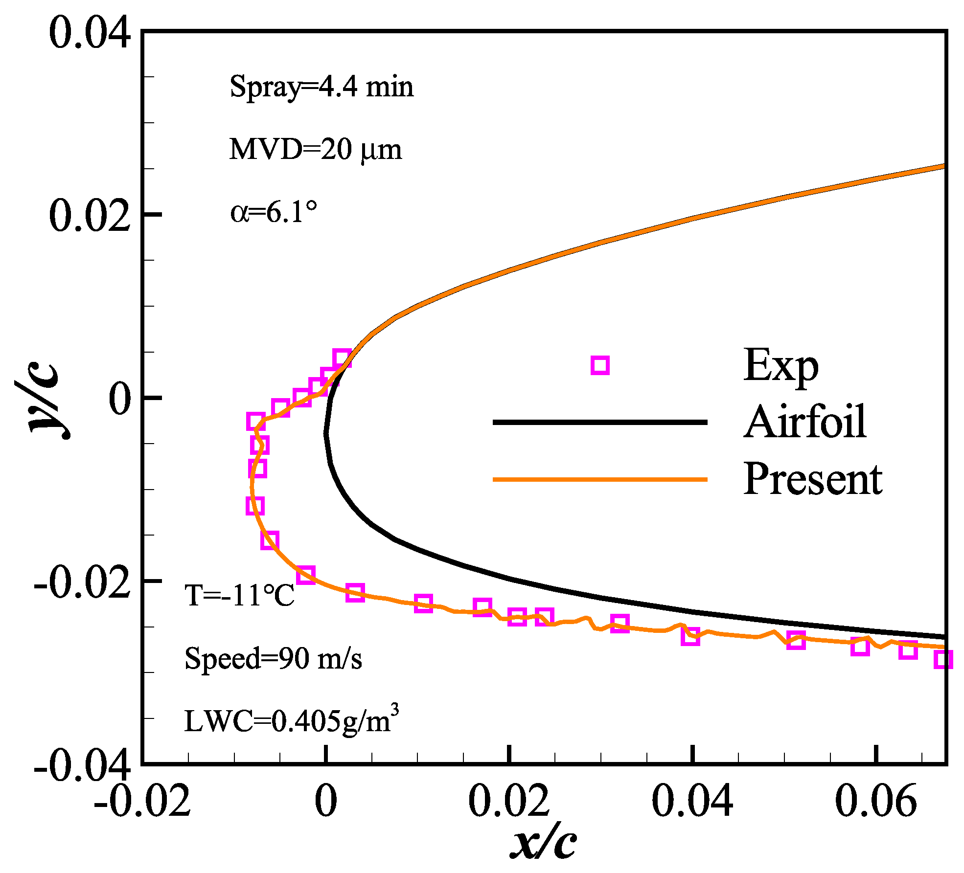
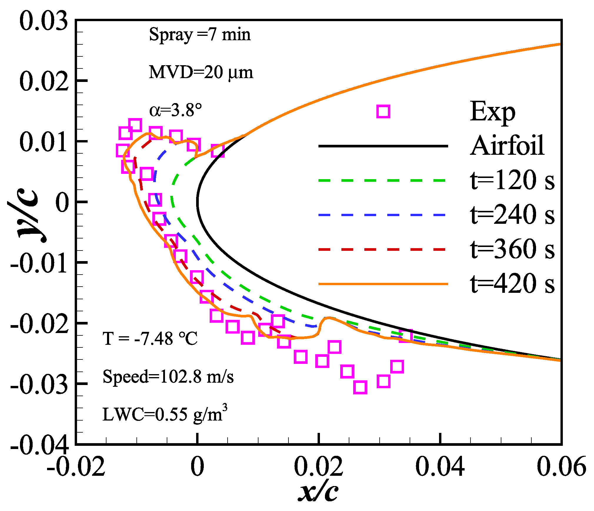
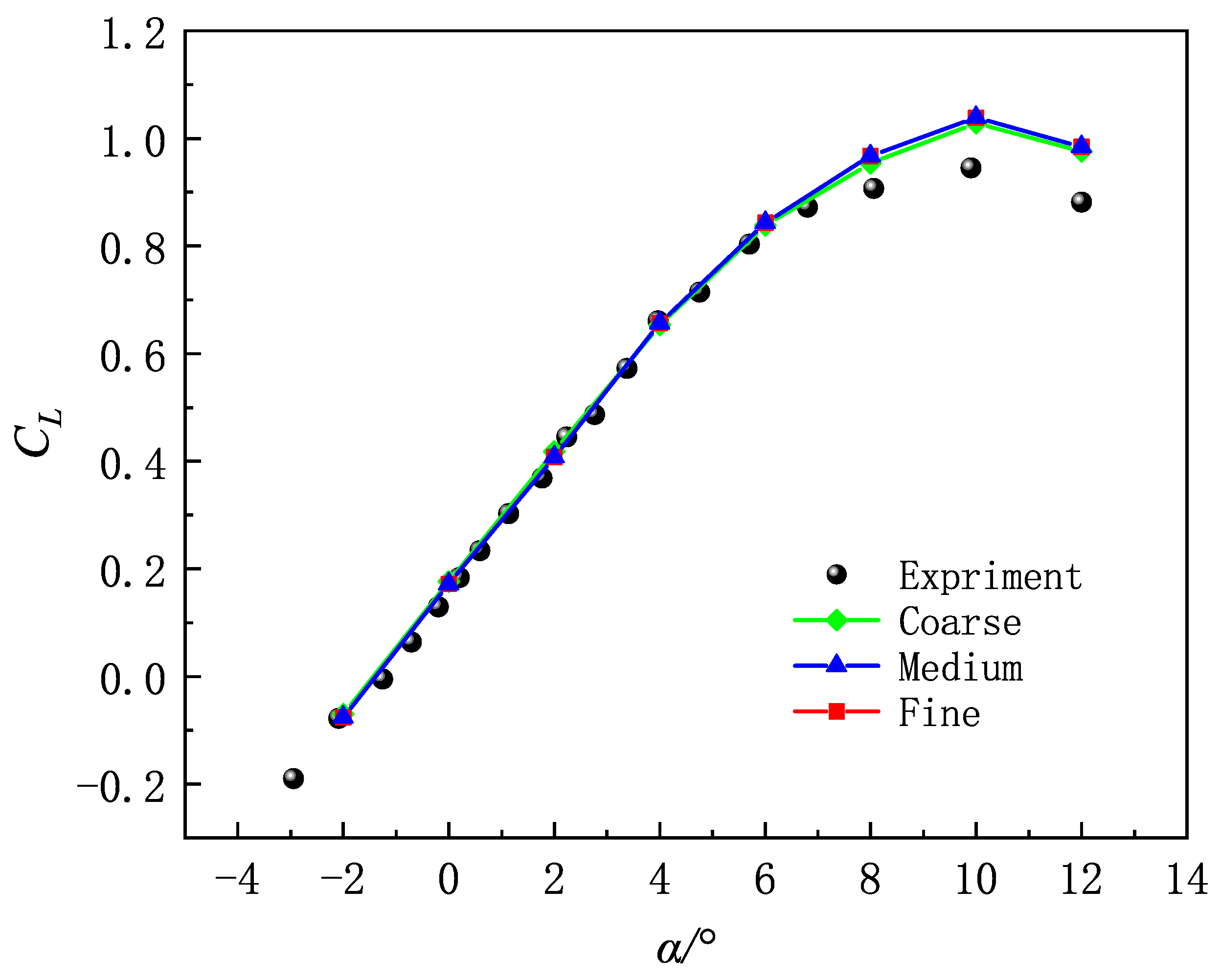
2.2. Method Verification

Numerical simulation of ice accumulation can be carried out in single and multi-step icing processes. Single-step icing can only approximate the main ice corners, while simulating glaze ice usually requires more than one step of icing to get a realistic profile of ice accretion [24]. Figure 1 and Figure 2 show the differences between the results of numerical simulations of ice accretion and experiments using the commercial jet airfoil GLC305 and the symmetrical airfoil NACA0012. The legend in the figure shows the static environment temperature, the LWC and MVD. In order to better fit the experiment results, the glaze ice calculation in Figure 2 use a multi-shot approach.

The rime ice calculations in Figure 1 show a great agreement with the experimental data, the horn-shaped glaze ice simulation in Figure 2 has a large profile difference on the lower surface of the airfoil. According to the reference [10], the horn-shaped ice profile can be characterized by the ice shape height and angle at the leading edge. Small difference exists between the starting angle and thickness of the upper ice angle and the experimental value. The angle of the upper ice has a profound effect on the flow field. The difference between the streamlined ice near the leading edge’s lower surface and the experimental value is within acceptable limits. Hence, the current numerical simulation method is deemed reliable.

3. Results and Discussion

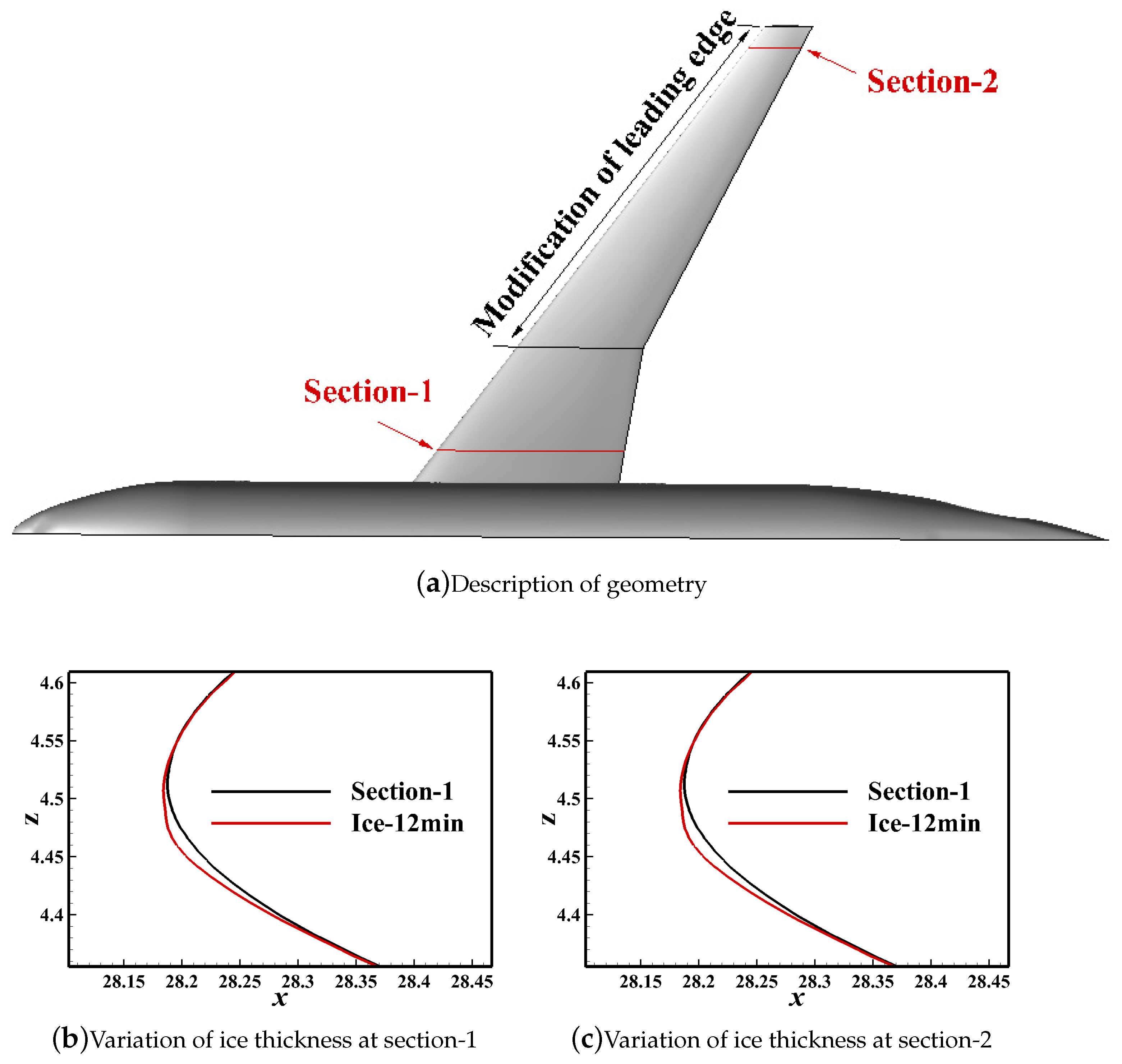
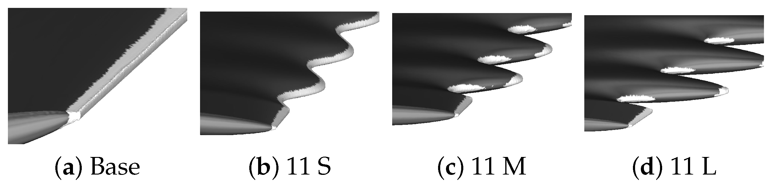
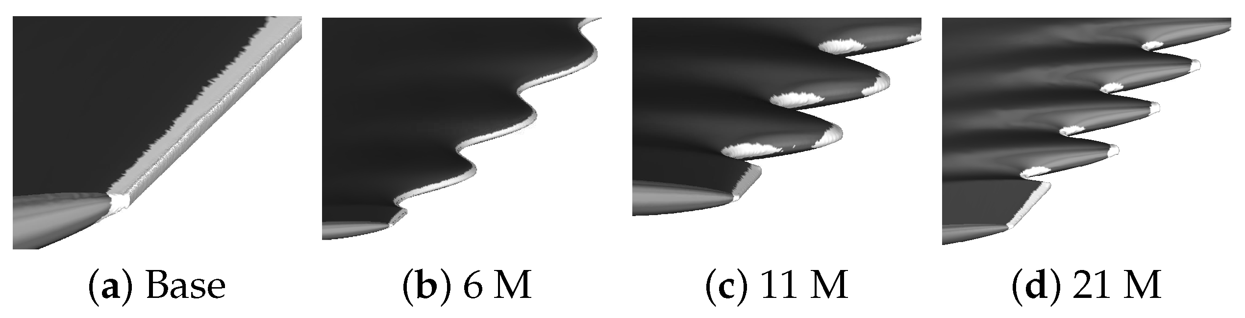
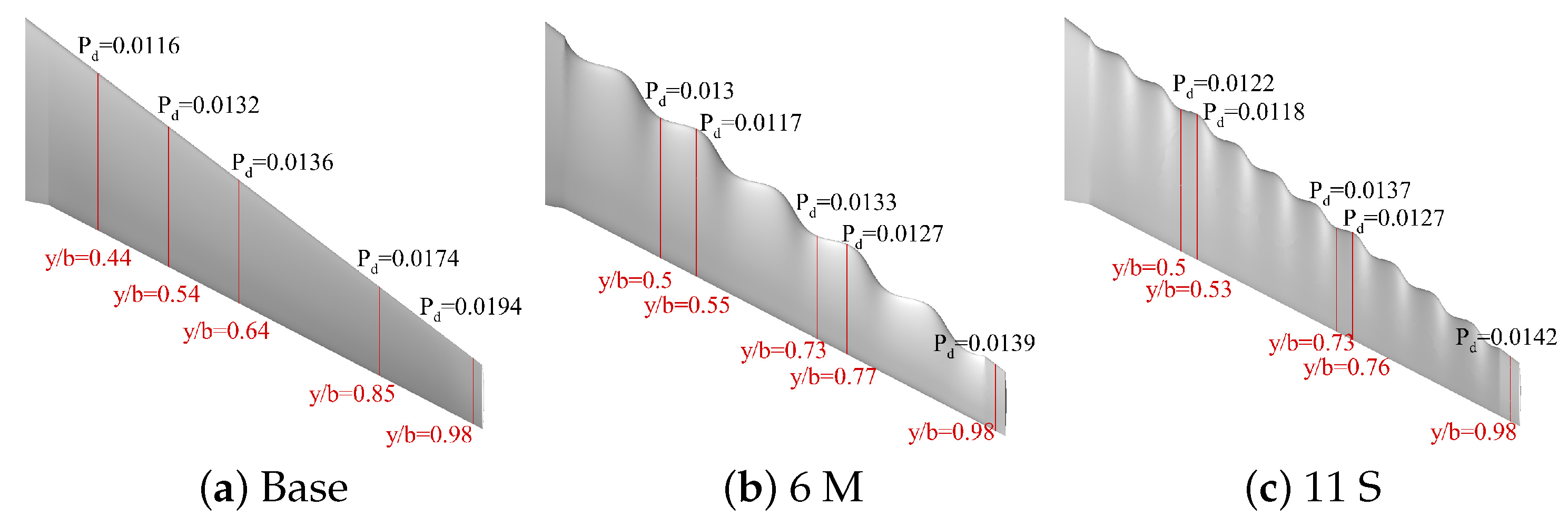
3.1. Geometry Description

The initial geometric model is the CRM [25], whose specific parameters are shown in

Table 1. Geometric parameters of the CRM.

Type	Value
Reference area (S)	383.6896 m2
Reference chord length (c)	7 m
Reference spanwise length (b)	58.8137 m

. A grid number irrelevance comparison is carried out in order to ensure the accuracy of the calculation and the requirements of the ice accretion simulation on the near-wall grid. The number of mesh cells are 4,127,890, 5,756,851 and 7,562,948, respectively, and the nondimensional distance of the first grid point away from the wall of all meshes is less than one. The freestream flow condition are $Ma=0.85$ and the Reynolds number is $Re=7\times {10}^7$ based on the reference chord length listed in Table 1. The flow solver is validated with all sets of mesh, and the results compared to the experimental values are shown in the Figure 3. The slope of lift curves from different meshes have a great match with the experimental data. In the further simulation, only the medium mesh will be use for a consideration of time cost.

Generally, rime ice is more regular in shape, has poor adhesion, and is prone to falling off. However, the glaze ice has an irregular form because the water droplets do not freeze completely. Backflow occurs frequently on a frozen surface and has a greater impact on aerodynamic changes [26]. For the current research, a horn-shaped ice with a high temperature was chosen for the subsequent calculation. The CRM wing has a significant anhedral angle as well as an installation angle. When the angle of attack is great, water droplets tend to flow along the lower surface of the wing towards the trailing edge of the wing, and ice builds up primarily on the lower surface of the leading edge of the wing, appearing as streamlined ice with no discernible ice angle. The angle of attack for ice accumulation is set to 2${}^{\circ }$, as smaller angles of attack make horn-shaped ice stand out more. The other flow conditions were v = 150 m/s, T = 268.15 K, MVD = 20 μm, LWC = 0.531433 g/m³, and the ice accretion time was 12 min. The single ice accumulation time was 3 min through a multi-step calculation, and a total of four calculations were made.

Horn-shaped ice will decrease the stall angle of attack and reduce flight safety, and the bionic leading edge generated by the vortex pair can delay the stall characteristics. Consequently, the leading edge of the wing is transformed into nodules of varying wavelengths and amplitudes. Figure 4 depicts the ice accretion shape of the initial model. As the radius of the leading edge of the wing increases, the thickness of the ice shape decreases, and the water droplet collection efficiency decreases significantly. Influenced by the spread flow and the radius of the leading edge, ice accretion is predominantly concentrated near the wingtip. Since the fin root of the humpback has a regular shape, the protuberance is primarily modified on the outer wing segment. The amplitudes and wavelengths of the protrusions refer to article [14]. The amplitudes selected for the model were 2.5% c, 5% c, and 10% c (c refers to the chord length). S, M, and L were used to represent the amplitudes, respectively. The wavelengths were 15% c, 30% c, and 50% c. The specific values of the three wavelengths were 1.05 m, 2.1 m and 3.5 m, and the corresponding wave numbers were 21, 11 and 6, respectively. Specific parameters are shown in

Table 2. Naming methods for models.

Label	Amplitude (A)	Wavelength ($\mathit{\lambda }$)
6 M	5 c	3.5 m
11 S	2.5 c	2.1 m
11 M	5 c	2.1 m
11 L	10 c	2.1 m
21 M	5 c	1.05 m

. Based on the medium grid chosen above, it takes 8 h to perform a single icing calculation using 64 CPUs.

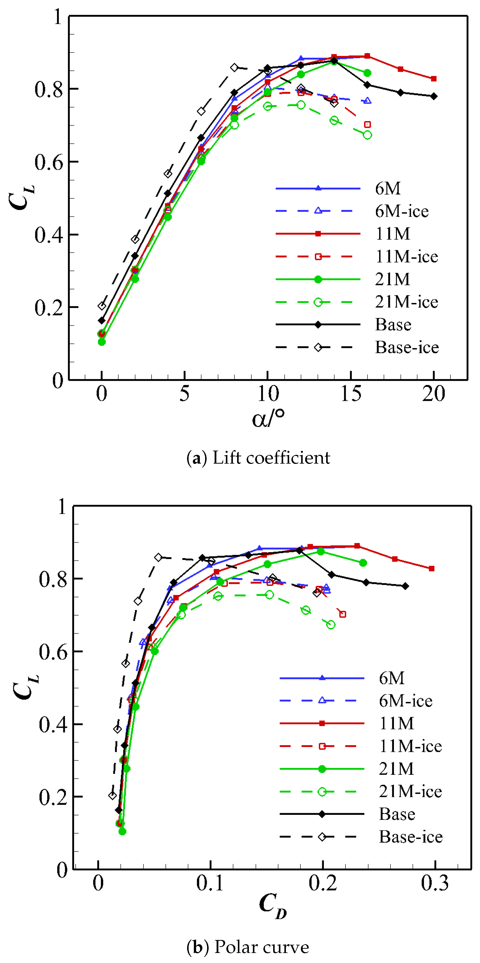
3.2. Effect of Amplitude

The changes in lift coefficient and polar curve before and after ice accretion in the initial CRM model and the modified model are shown in Figure 5. The effective chord length and the leading edge curve of the airfoil at the wing tip both increase due to the increse of ice accretion thickness at the leading edge. The lift coefficients of the ice-accretion model (Base-ice) before the stall angle of attack are greater than those of the initial model (Base). The reason for the decrease in drag coefficient after ice accretion may be that the roughness of ice accumulation at the leading edge of the outer wing segment changes, the airflow contact area decreases, and the friction resistance decreases at this temperature.

The asymmetry of the upper and lower ice angles near the wing tip easily leads to a large separation area on the upper surface, as shown in Figure 6. As the downwash effect decreasing, the pressure drag becomes lower due to the smaller wing-tip vortex [27]. In Figure 6, the area of the pressure distribution can be projected to the streamwise direction, that is, the pressure drag of the base model is larger than that of the one with ice. In the case with ice, the lift coefficient of the configuration increases a little. However, the stall angle of attack decreases from 14${}^{\circ }$ to 8${}^{\circ }$. Commonly, ice accretion on the airplane have a intensive effect on the aerodynamic performance such as reducing the stall angle. The horn-shaped ice has a strong relation with the ice accreting time, hence the special phenomenon that the lift increases and the drag decreases in present study can be regarded as a coincidence. Therefore, the following discussion will mainly be concentrated on the stall feature of the wing.

As shown in Figure 7, the ice accretion on the different leading edges of the wing is given. The larger peak of nodules, the more nonuniformity of the ice (denoted with the white color) on the wing, compared to the base model. Although the protuberance of the leading edge deteriorates the lift coefficients, the stall angle is kept with that of the base model without ice. The wavy leading edge with larger amplitude gives lower droplet collection efficiency regarding to the amount of the ice over the wing surfaces. The discontinuous distribution of ice gives a better recovery of the original shape of the wing. Moreover, the maximum reduction in lift coefficient is not more than 10%, compared with the base model. With ice accretion, the value of lift coefficients have a 7% decrease for 11 L, and 1.5% and 6% increases for 11 M and 11 S, respectively. All results indicate that the amplitude of the nodules will suppress the ice increment, which, certainly, will have much benefit on the aerodynamic performance at stall condition. The best capability of ice suppression is given by 11 S.

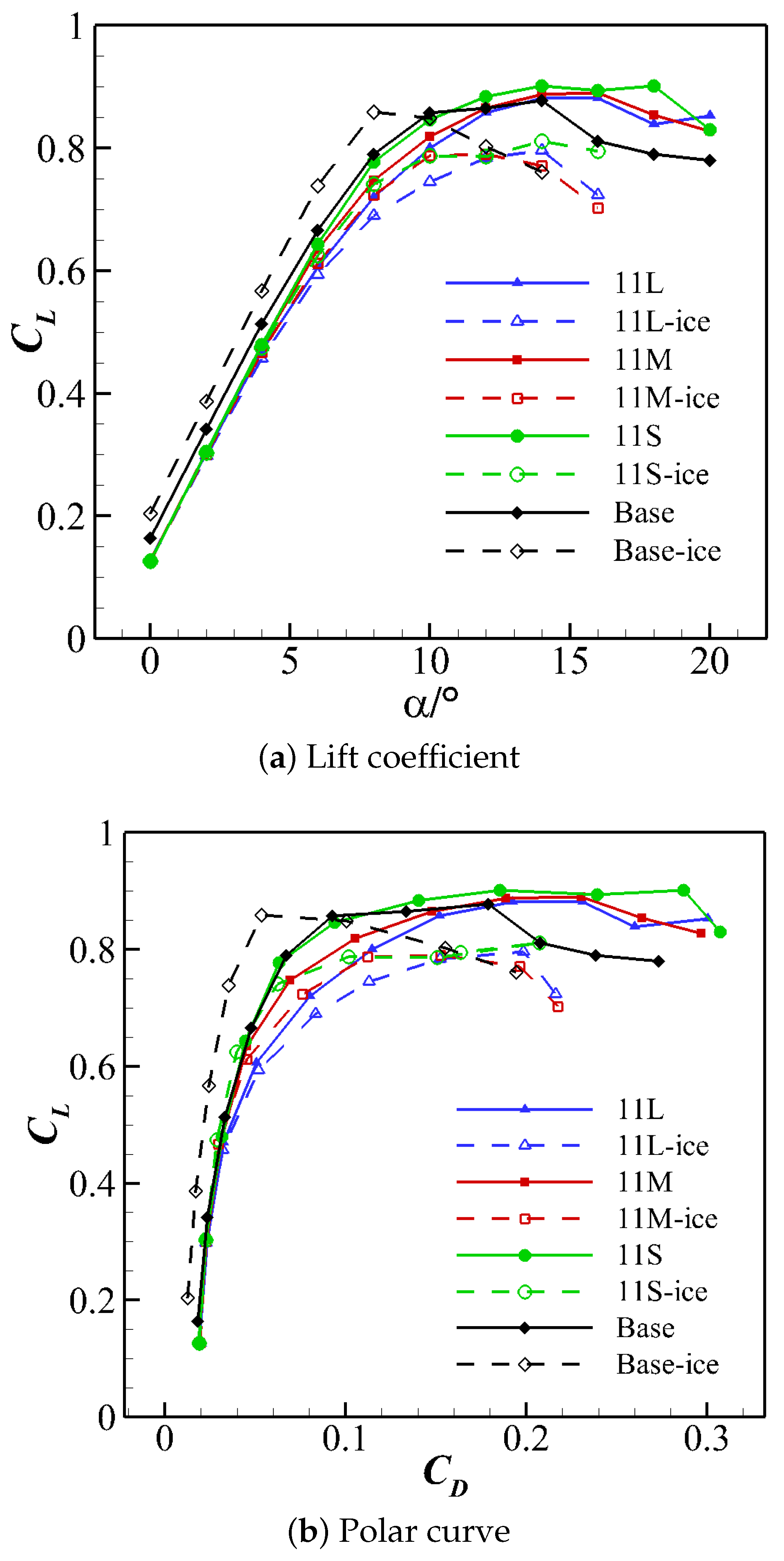
3.3. Effect of Wavelength

The current section will discuss the effect of the wavelength of the leading edge protrusion, and the the amplitude of wavy edge is kept to be 5%c. The lift coefficients and polar curve of the models are plotted in Figure 8. Among the model with ice, 6 M has the highest lift coefficient, with just slight drop as the wavelength increase to 11, i.e., the model 11 M. With the increase of wave number, the lift coefficient of 21 M is reduced compared with that of the base model when the wing is not frozen, and the maximum reduction is as much as 35% at an angle of 0${}^{\circ }$. The drag coefficient is the same as that of the base model only at an angle of 4${}^{\circ }$, while at other angles of attack it is greater. No matter how the leading edge geometry changes, the optimum angle of attack can be maintain at an angle of 4${}^{\circ }$. The geometric shape changes of the leading edge after ice accretion are shown in Figure 9. The thickness of the 6 M ice shape seems to be continuous ice with uniform thickness, and the maximum thickness of the ice is much smaller than that of the base model. The ice formations at 11 M and 21 M are clearly discontinuous ice. The curvature at the crest of 21 M is very small, resulting in a large thickness of the ice. As a result, the long wavelength can reduce the amount of ice accretion and prevent aircraft from stalling at a small angle of attack.

Based on the change of lift coefficient and maximum lift-to-drag ratio, the present study analyzes the aerodynamic changes of protrusions with different amplitudes and wavelengths before and after ice accumulation. The influence mechanism and specific changes in ice type at the leading edge are not clearly explained.

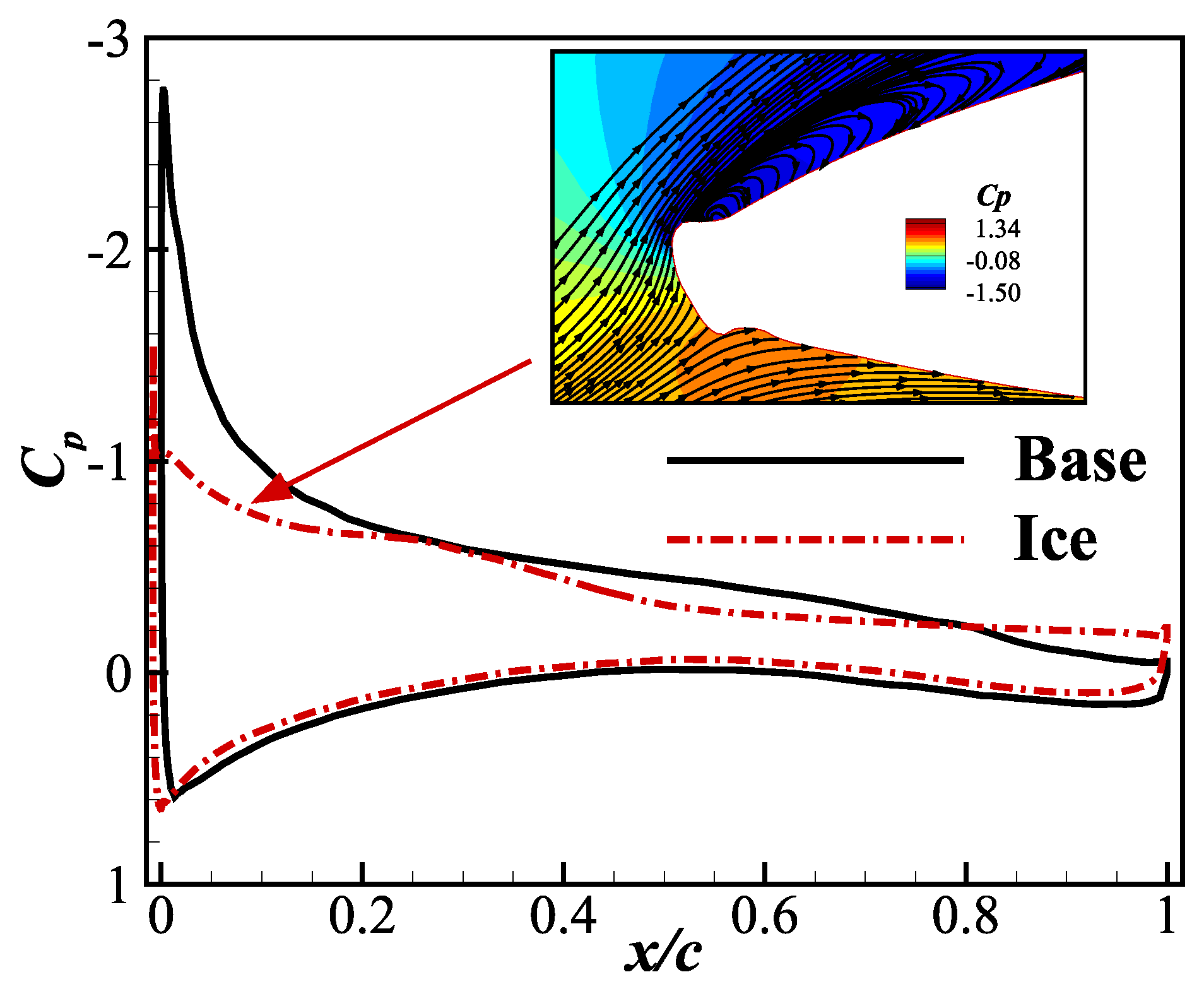
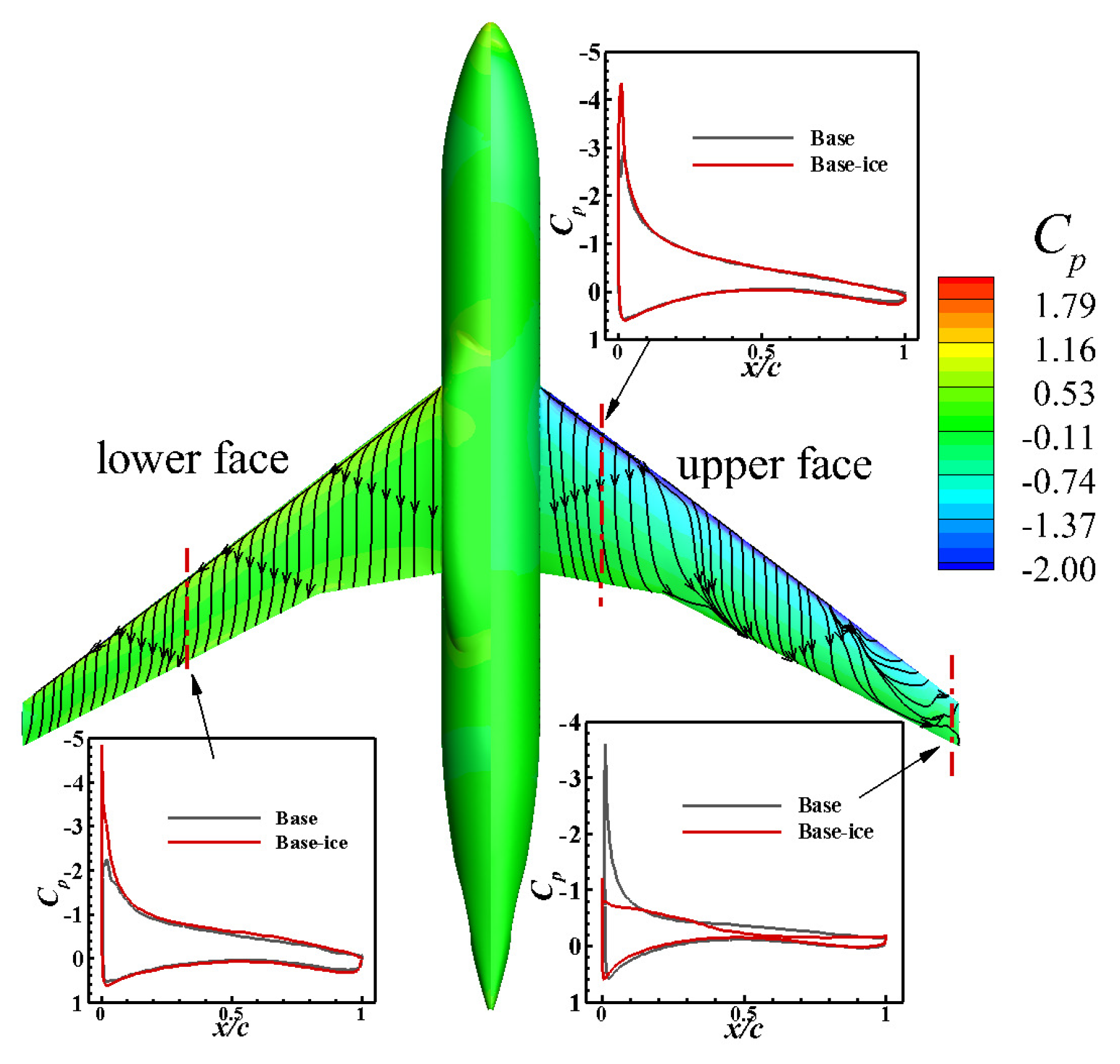
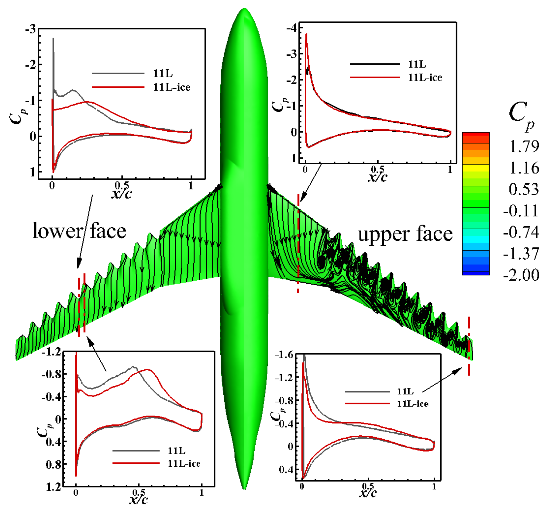
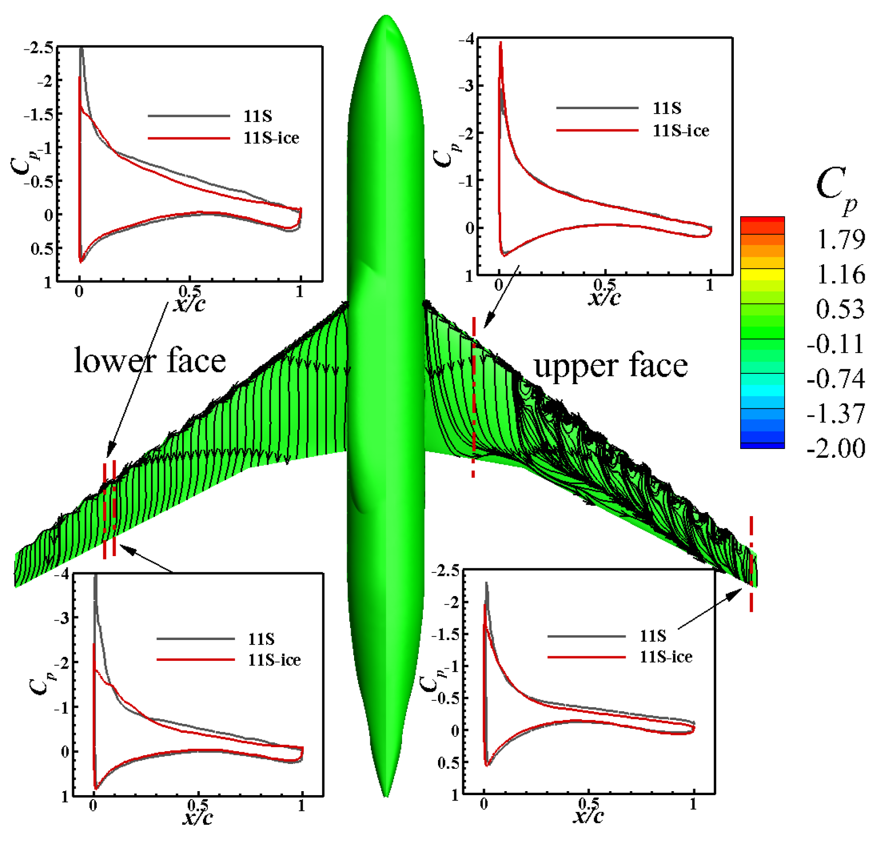
3.4. Analysis of Flow Field

Four models, Base, 11 L, 11 S, and 6 M, were chosen to evaluate the streamtraces of the leading edge after freezing at an angle of attack of 8${}^{\circ }$ and to compare the pressure coefficient curve differences induced by the leading edge modification and ice formation. The positions of different sections are shown in Figure 10, Figure 11, Figure 12 and Figure 13. By changing the leading edge of the outer wing segment, the protuberance with different amplitudes and wavelengths can relieve the pressure distribution changes after ice formation, which is indicated with the surface pressure contour similarity of all models in Figure 10. The change of leading edge protuberance has obvious influence on the pressure distribution after icing, especially the change of suction surface [28]. It should be noted that the angle of attack of 8${}^{\circ }$ is the stall angle of attack after ice builds up in the base, while the value of the other three models is still larger than 8${}^{\circ }$, and the protrusion obviously delays the stall characteristic. In Figure 11, Figure 12 and Figure 13, a cluster of counter-rotating vortex pairs at the nodule are obvious. These vortices bring extra energy from the flow far away from the boundary layer. The corresponding pressure distribution at the peak and trough are also given in the figure. Combined with Figure 5 and Figure 8, 11 L has a lower lift coefficient than 6 M and 11 S before the stall angle of attack, including the findings after icing. Due to the large number of protuberance in 11 L, the counter-rotating vortex pairs will lose some energy in the air flow, and the lift coefficient is slightly reduced. The size of leading edge vortex over both 6 M and 11 S are small, and the lift coefficient are similar with that of Base. The drag coefficient of 11 S is higher than those of the other three models whether ice does accrete or not. However, the stall angle of attack can be kept at 14${}^{\circ }$ without much change from ice formation. The stall angle of attack before and after 6 M ice accumulation is 12${}^{\circ }$ and 10${}^{\circ }$, respectively, and its ability to delay stall is weak. The lift and drag coefficient of 11 S are not significantly different from that of 6 M, but the stall angle of attack can be maintained at 14${}^{\circ }$ before and after ice accumulation, which can relieve the stall. The 11 S has the nearest aerodynamic performance with the Base when there is no ice on the wing, and the stall angle is kept at the same time. Therefore, out of the three different parameters of the nodule model, 11 S has the best effect.

3.5. Procrustes Analysis

Procrustes analysis is a tool used in statistics for multivariate analysis. It is often used to study the shape statistically [18,19]. The object’s position and size can be changed in any way to make the Procrustes distance ($P_d$) as small as possible via translation, rotation, and scaling. Based on wavelength and amplitude, the model with best aerodynamic performance is selected herein. The airfoil profiles at five different places, on the outer segment of Base, 6 M and 11 S model were chosen. Among them, 6 M and 11 S are, respectively at the peak and trough of the wave, and the common cross-sectional position of all models is $y/b=0.98$ near the wing tip. According to the airfoil curves at different span positions of the model before and after ice accumulation, the overlapping parts were removed, and only the shape with obvious ice accretion thickness at the leading edge was retained. The key points of the initial airfoil were found based on the ordinate of the ice-type data points. After data transformation, it is divided by $k^2$ to reduce the influence caused by the number of different data points. The formula is as follows:

$$k^2{P_d}^2=\sum _{i=1}^k[{(x_{i1}-x_{i2})}^2+{(y_{i1}-y_{i2})}^2]$$

(6)

The Procrustes distances at different cross sections are shown in Figure 14. The smaller the $P_d$ value is, the higher the contour coincidence degree of the leading edge before and after ice accretion is, which means the smaller the ice type thickness is.

The $P_d$ of Base gradually increased along the span direction, and the ice accretion thickness was the largest at the wing tip. The $P_d$ of 11 S shows an increasing trend from peak to trough, which proves that the ice accretion thickness of the peak is smaller than that of the trough. The variation of $P_d$ from peak to trough of 6 M is the same as that of 11 S. Compared with the leading edge profile of the base model, the change in the leading edge protrusion is small. The sum of the $P_d$ of the five cross sections in 6 M is close to the size of 11 S. At spanwise $y/b=0.98$, the $P_d$ of the three models are 0.0194, 0.0139, and 0.0142, respectively. This shows that the protuberance effectively weakens the ice accretion near the wing tip, and the spanwise continuous ice becomes relatively safe discontinuous ice. Comprehensive analysis shows that the anti-icing performance of 6 M and 11 S are similar, that is, both of them can effectively reduce the thickness of ice that builds up at the leading edge.

4. Conclusions

In this work, a bio-inspired leading edge is presented as a means of preventing wing icing. Using a comparison of amplitudes and wavelengths, the aerodynamic properties prior to and after ice accretion were investigated. It has been discovered that protuberance can effectively limit the ice formation at the leading edge and prevent the stall. By examining the flow field, the changes of vortices at the leading edge are given. Vortices are proportional to the amplitude and wavelength of protuberances. The 11 S has good aerodynamics both before and after ice formation, with the same angle of attack at stall as before ice formation. Lastly, taking Base, 6 M, and 11 S as examples, the thickness changes of ice types are quantified based on the changes in the leading edge’s shape before and after ice accretion. It is less likely that the aerodynamic properties of discontinuous ice will deteriorate than those of continuous ice. This demonstrates that the bionic leading edge can prevent ice accretion to some extent and provides researchers with a novel design concept for the anti-icing device. Future research will continue to examine how ice forms and melts at the peaks and valleys of nodules, as well as how the surface roughness of different types of ice varies, in order to develop a more effective bio-inspired leading edge for anti-icing.

References

1. Addy, H.E. Ice Accretions and Icing Effects for Modern Airfoils; National Aeronautics Administration, Glenn Research Center: Washington, DC, USA, 2000. [Google Scholar]
2. Hassan, N.; Lu, S.; Xu, W.; He, G.; Faheem, M.; Ahmad, N.; Khan, M.A.; Butt, B.Z. Fabrication of a Pt nanoparticle surface on an aluminum substrate to achieve excellent superhydrophobicity and catalytic activity. New J. Chem. 2019, 43, 6069–6079. [Google Scholar] [CrossRef]
3. Annavarapu, R.K.; Kim, S.; Wang, M.; Hart, A.J.; Sojoudi, H. Explaining evaporation-triggered wetting transition using local force balance model and contact line-fraction. Sci. Rep. 2019, 9, 405. [Google Scholar] [CrossRef] [PubMed] [Green Version]
4. Khadak, A.; Subeshan, B.; Asmatulu, R. Studies on de-icing and anti-icing of carbon fiber-reinforced composites for aircraft surfaces using commercial multifunctional permanent superhydrophobic coatings. J. Mater. Sci. 2021, 56, 3078–3094. [Google Scholar] [CrossRef]
5. Ma, L.; Li, H.; Hu, H. An Experimental Study on the Dynamics of Water Droplets Impingement onto a Goose Feather. In Proceedings of the 55th AIAA Aerospace Sciences Meeting, Grapevine, TX, USA, 9–13 January 2017; p. 442. [Google Scholar]
6. Alizadeh-Birjandi, E.; Tavakoli-Dastjerdi, F.; Leger, J.S.; Faull, K.F.; Davis, S.H.; Rothstein, J.P.; Pirouz Kavehpour, H. Delay of ice formation on penguin feathers. Eur. Phys. J. Spec. Top. 2020, 229, 1881–1896. [Google Scholar] [CrossRef]
7. Diebold, J.M.; Broeren, A.P.; Bragg, M. Aerodynamic classification of swept-wing ice accretion. In Proceedings of the 5th AIAA Atmospheric and Space Environments Conference, San Diego, CA, USA, 24–27 June 2013; p. 2825. [Google Scholar]
8. Broeren, A.P. Swept-Wing Ice Accretion Characterization and Aerodynamics: Research Plans and Current Status. In Proceedings of the 2011 Annual Technical Meeting, St. Louis, MO, USA, 10–12 May 2011. [Google Scholar]
9. Li, H.R.; Zhang, Y.F.; Chen, H.X. Optimization design of airfoils under atmospheric icing conditions for UAV. Chin. J. Aeronaut. 2022, 35, 118–133. [Google Scholar]
10. Li, H.; Zhang, Y.; Chen, H. Optimization of supercritical airfoil considering the ice-accretion effects. AIAA J. 2019, 57, 4650–4669. [Google Scholar] [CrossRef]
11. Yirtici, O.; Tuncer, I.H.; Ozgen, S. Aerodynamic shape optimization of wind turbine blades for reducing power production losses due to ice accretion. In Proceedings of the 35th Wind Energy Symposium, Grapevine, TX, USA, 9–13 January 2017; p. 1850. [Google Scholar]
12. Zhang, Y.; Zhang, X.; Li, Y.; Chang, M.; Xu, J.K. Aerodynamic performance of a low-Reynolds UAV with leading-edge protuberances inspired by humpback whale flippers. Chin. J. Aeronaut. 2021, 34, 415–424. [Google Scholar] [CrossRef]
13. Chen, H.; Pan, C.; Wang, J. Effects of sinusoidal leading edge on delta wing performance and mechanism. Sci. China Technol. Sci. 2013, 56, 772–779. [Google Scholar] [CrossRef]
14. Gopinathan, V.; Bruce Ralphin Rose, J. Aerodynamics with state-of-the-art bioinspired technology: Tubercles of humpback whale. Proc. Inst. Mech. Eng. Part J. Aerosp. Eng. 2021, 235, 2359–2377. [Google Scholar] [CrossRef]
15. Johari, H.; Henoch, C.; Custodio, D.; Levshin, A. Effects of leading-edge protuberances on airfoil performance. AIAA J. 2007, 45, 2634–2642. [Google Scholar] [CrossRef]
16. Cai, C.; Zuo, Z.; Maeda, T.; Kamada, Y.; Li, Q.; Shimamoto, K.; Liu, S. Periodic and aperiodic flow patterns around an airfoil with leading-edge protuberances. Phys. Fluids 2017, 29, 115110. [Google Scholar] [CrossRef]
17. Miklosovic, D.S.; Murray, M.M.; Howle, L.E. Experimental evaluation of sinusoidal leading edges. J. Aircr. 2007, 44, 1404–1408. [Google Scholar] [CrossRef]
18. Gower, J.C. Generalized procrustes analysis. Psychometrika 1975, 40, 33–51. [Google Scholar] [CrossRef]
19. Meyners, M.; Kunert, J.; Qannari, E.M. Comparing generalized procrustes analysis and STATIS. Food Qual. Prefer. 2000, 11, 77–83. [Google Scholar] [CrossRef] [Green Version]
20. Bourgault, Y.; Beaugendre, H.; Habashi, W.G. Development of a shallow-water icing model in FENSAP-ICE. J. Aircr. 2000, 37, 640–646. [Google Scholar] [CrossRef]
21. Beaugendre, H.; Morency, F.; Habashi, W. ICE3D, FENSAP-ICE’S 3D in-flight ice accretion module. In Proceedings of the 40th AIAA Aerospace Sciences Meeting & Exhibit, Reno, NV, USA, 14–17 January 2002; p. 385. [Google Scholar]
22. Morency, F.; Beaugendre, H.; Habashi, W. FENSAP-ICE: A Navier-Stokes Eulerian Droplet Impingement Approach for High-Lift Devices. CASI Conf. 2001, 15, 16. [Google Scholar]
23. Ozcer, I.A.; Baruzzi, G.S.; Reid, T.; Habashi, W.G.; Fossati, M.; Croce, G. Fensap-Ice: Numerical Prediction of Ice Roughness Evolution, and Its Effects on Ice Shapes; SAE Technical Paper, 2011-38-0024; SAE International: Warrendale, PA, USA, 2011. [Google Scholar] [CrossRef]
24. Pena, D.; Hoarau, Y.; Laurendeau, E. A single step ice accretion model using Level-Set method. J. Fluids Struct. 2016, 65, 278–294. [Google Scholar] [CrossRef] [Green Version]
25. Vassberg, J.; Dehaan, M.; Rivers, M.; Wahls, R. Development of a common research model for applied CFD validation studies. In Proceedings of the 26th AIAA Applied Aerodynamics Conference, Honolulu, HI, USA, 18–21 August 2008; p. 6919. [Google Scholar]
26. Çakir, T. Evaluation of Ice Accretion on a 2D Airfoil Using Commercial and Open Software. 2018. Available online: http://essay.utwente.nl/85119/ (accessed on 30 January 2018).
27. Bolzon, M.; Kelso, R.; Arjomandi, M. The effects of tubercles on swept wing performance at low angles of attack. In Proceedings of the 19th Australasian Fluid Mechanics Conference, Melbourne, Australia, 8–11 December 2014; pp. 8–11. [Google Scholar]
28. Pillai, S.N.; Sundaresan, A.; Gopal, R.; Priya, S.; Pasha, A.A.; Hameed, A.Z.; Jameel, A.G.A.; Reddy, V.M.; Juhany, K.A. Estimation of Chaotic Surface Pressure Characteristics of Ice Accreted Airfoils–A 0–1 Test Approach. IEEE Access 2021, 9, 114441–114456. [Google Scholar] [CrossRef]
Figure 1. Rime ice condition.
Aerospace 09 00774 g001
Figure 2. Glaze ice condition.
Aerospace 09 00774 g002
Figure 3. Verification of different number of grids.
Aerospace 09 00774 g003
Figure 4. The shape change of the CRM wing’s leading edge after ice accretion and the description of the bionic leading edge position.
Aerospace 09 00774 g004
Figure 5. Effect of amplitude variation on lift and drag coefficients.
Aerospace 09 00774 g005
Figure 6. Pressure distribution and streamline changes at y / b = 0.95 .
Aerospace 09 00774 g006
Figure 7. Changes in ice accumulation at the leading edge of different amplitudes.
Aerospace 09 00774 g007
Figure 8. Effect of wavelength variation on lift and drag coefficients.
Aerospace 09 00774 g008
Figure 9. Changes in ice accumulation at the leading edge of different wavelengths.
Aerospace 09 00774 g009
Figure 10. Flow field changes of Base before and after ice accumulation.
Aerospace 09 00774 g010
Figure 11. Flow field changes of 11L before and after ice accumulation.
Aerospace 09 00774 g011
Figure 12. Flow field changes of 11S before and after ice accumulation.
Aerospace 09 00774 g012
Figure 13. Flow field changes of 6M before and after ice accumulation.
Aerospace 09 00774 g013
Figure 14. Procrustes distance at different cross sections.
Aerospace 09 00774 g014