Simulation of Forced Convection Frost Formation in Microtubule Bundles at Ultra-Low Temperature

Abstract

Hypersonic vehicles are an important area of research in the aerospace field today. One of the important issues is the power of the engine. In order to achieve large-span flight speeds, a more efficient approach is to use combined power systems. However, the problem of pre-cooler icing can occur in combined engine applications. The flow in the pre-cooler is extremely complex. Outside the tube is the high-temperature wet air entering from the engine intake, and the tube cooling is the ultra-low temperature cooling medium. Icing not only increases the heat exchange resistance of the pre-cooler during operation and affects the heat exchange performance of the pre-cooler, but also causes a large total pressure loss, resulting in a degradation of the engine performance. There is a lack of research on the icing law of the pre-cooler under different parameters. Therefore, it is necessary to conduct a corresponding numerical calculation study on pre-cooler icing and explore the influence of various influencing factors on icing. In this paper, a mathematical model of icing (frost) is established for the frosting phenomenon that may occur during the operation of the pre-cooler. Additionally, the principle of heat and mass transfer in the icing process is described by the mathematical model, and the influence of different parameters on the frosting parameters is explored by using the computational fluid dynamics (CFD) method. The law of tube bundle icing under different parameters was calculated, and the variation laws of frost layer morphology and wet air pressure drop were obtained. The laws of tube bundle icing under different parameters were calculated, and the changes in frost layer pattern and wet air pressure drop when each parameter was changed, which can provide guidance for the design and application of pre-coolers in the future.

1. Introduction

With the use of ultra-low temperatures in industrial production and aerospace applications, the frosting that can occur on cryogenic surfaces during application is of increasing concern. For example, as liquefied natural gas (LNG) [1,2,3] has become more widespread, LNG vaporization units have evolved. Ambient air vaporizers (AAVs) [4,5,6,7], which utilize the atmosphere as a heat source to vaporize liquid natural gas, may experience surface frosting during operation. For cryogenic oxidizer tanks of liquid propulsion rockets [8], frost forms due to phase change deposition of water vapor, on the surface when moist air comes in contact with the tank surface at temperatures below 273 K. To solve the power problem of hypersonic vehicles, the inlet pre-cooling is used to extend the thrust range of the combined engine [9,10,11,12,13]. A pre-cooler is used to cool the gases entering the combined engine from the engine intake. The cooling medium in the pre-cooler is usually liquid helium, liquid hydrogen, etc. During the flight of the aircraft from the ground to an altitude of 12 km, the water vapor in the air undergoes a phase change as the air temperature decreases and forms a frost layer on the surface of the pre-cooler tube bundle.

Frost occurs on the surface of the micro-tube bundle of the pre-cooler because the surface of the tube bundle is kept at a low temperature during the operation of the pre-cooler. Additionally, existing studies have shown that frost on the tube bundle surface will seriously reduce the heat exchange efficiency and the total pressure recovery coefficient [14] after heat exchange during pre-cooler operation, which in turn will deteriorate the overall engine performance. Frost is considered to be a porous medium consisting of moist air and ice crystals, and the effective thermal conductivity of the frost layer is usually very low due to its high porosity. Additionally, the growth of the frost layer changes the cross-sectional area of wet air circulation in the pre-cooler. To predict the frost growth, we need to determine the mass transfer rate of wet air to the frost layer, the mass diffusivity in the frost layer, and various physical properties of the frost layer. Hayashi et al. [15] divided the evolution of frost layer growth into three periods: crystal growth period, frost layer growth period, and frost complete growth period.

The existing models for predicting frost growth can be divided into theoretical analysis and CFD (computational fluid dynamics) numerical simulations. The theoretical analysis mainly uses programming methods combined with various empirical formulas and assumptions to predict the thickness and density of frost growth, mainly for one-dimensional problems. Jung Soo Kim and Kwan Soo Lee [16] proposed a mathematical model to predict the frost on heat exchanger fins under frost conditions. The heat conduction of fins is considered and a correlation method to predict the equivalent temperature is proposed to improve the accuracy of frost prediction. Sangho Choi and Sung Jin Kim [17] studied the effect of wall temperature on surface heat and mass transfer under natural convection conditions and proposed a numerical model for frosting considering initial wall cooling, and the maximum and minimum heat fluxes obtained from the model were in good agreement with experimental data within 10% and 25% error, respectively. The frost layer thickness is within 13% error with experimental data. Dong Keun Yang and Kwan Soo Lee [18] proposed a dimensionless correlation to predict the properties of frost formed on a cold plate. The correlations with various environmental parameters were obtained through frosting experiments. The thickness, density, surface temperature, and other variables of the frost layer were correlated as a function of the Reynolds number, Fourier number, absolute humidity, and dimensionless temperature using the dimensional analysis method. Additionally, the proposed model calculations agreed well with the experimental data with a maximum error of 10%. Christian J.L. Hermes [19] proposed an algebraic first-principles simulation model to predict the growth and density of frost layers on a flat surface. The model is based on macroscopic heat and mass balances in the frost layer and is prepared and solved analytically according to dimensionless formulas to obtain an algebraic expression for the time evolution of frost layer thickness with Nussle number, supersaturation, and temperature difference, the calculated results agree well with the measured results. R.Le Gall and J. M. Grillot [20] proposed a frost model based on a one-dimensional transient formulation to predict frost growth and densification when wet air outgrows the flat plate, proposing a new expression for the diffusive drag coefficient.

The frosting mechanism was studied by CFD and a mathematical model of the phase change mass transfer of the frosting process was developed, which is based on the criteria of frost growth and densification process and by simulating the frost growth on a locally cooled cold surface using Computational Fluid Dynamics (CFD) software. Sungjoon Byun, Haijun Jeong, et al. [21] developed a frosting model for predicting frosting behavior under low-temperature conditions. In their study, the Stefan number (STE) was used to define the mass transfer rate. The frosting behavior was visualized by numerical analysis and the results were compared with experimental data to verify the validity of the model. A relatively low-density frost layer was calculated to form at low temperatures, with a condensation-based frosting mechanism, and the frost density distribution of internal frosting was quantified. J. Cui, W.z. Li, Y. Liu [22,23] proposed a new CFD model to predict frost formation and growth using nucleation theory. The model can be used to describe the initial and growth periods of frost formation, reflects the influence of surface structure on frost development, and predict the time and space variation of frost structure and its characteristics. The model is used to simulate frost phenomena in plate cold surfaces and finned-tube heat exchangers. The simulation results were compared with the experimental results and data calculated by empirical equations to obtain transient localized frosting. The average frost thickness, heat exchanger coefficient, and air-side pressure drop were analyzed. Jaehwan Lee, Junghan Kim, et al. [24] proposed a numerical model for frost growth prediction based on computational fluid dynamics that can predict the growth behavior of high porosity frost formed by water vapor sublimation and a new volumetric mass transfer rate equation that takes into account the permeability of water vapor in the frost layer. The model is validated by experimental results and used to analyze the frost growth process. Donghee Kim, Chiwon Kim [25], proposed a CFD-based model to predict macroscopic and local frost behavior on a cold plate. Various factors affecting frost formation, including inlet velocity, relative humidity, and cold plate temperature, were verified and investigated by comparing them with experimental data. The numerical prediction results are in good agreement with the experimental data. It can be known that the method of theoretical analysis mainly relies on various existing empirical formulas for frost density, thickness, thermal conductivity, etc., and requires initial assumptions on the initial thickness and density of the frost layer. The numerical calculation method needs to establish the mass transfer coefficient and frost criterion, which is suitable for two-dimensional and three-dimensional frost problems, has a greater advantage for frost problems on complex structures, and can visualize the frosting process.

With the application and development of ultra-low temperatures in various fields, the environment where frosting occurs is becoming more and more complex. Additionally, the existing frosting models are not accurate in predicting frosting at ultra-low temperatures. The pre-cooler is composed of micro-tubes with a diameter of 1–2 mm and the tube bundle structure is in horizontal rows. Therefore, during the operation of the pre-cooler, the frost on the tube wall is more complicated by the tube bundle structure and operating conditions than the frost that occurs in other applications. Additionally, the frost layer that appears will affect the performance of the pre-cooler in several ways.

Considering the special characteristics of the pre-cooler tube bundle structure, this paper establishes the mass transfer equation based on the existing CFD model using the supersaturation of wet air. Additionally, combined with the critical density and ice phase volume change rate to obtain the ultra-low temperature surface frosting criterion. The surface frosting model of the ultra-low temperature tube bundle under forced convection was established. The heat and mass transfer occurring during the frosting process is simulated by adding the corresponding user-defined function (UDF) source terms to each control equation. The morphology of frosting on the surface of microtubular bundles at ultra-low temperatures and the effect of frosting on the pressure drop of humid air are investigated. The effects of different factors (cooling medium temperature, wet airflow velocity, moisture content) on the frost morphology of microtubular bundles and the pressure drop of wet air are also investigated.

2. Mathematical Modeling and Methods

When moist air comes in contact with a surface with a temperature below the freezing point, moisture will condense on the surface, and frost will occur. The frosting process will involve mass and heat transfer between the moist air and the frost layer, so the accuracy of these two parameters has a crucial impact on predicting the development of frosting. Current research divides the frosting process on cold surfaces into three characteristic periods: the crystal growth period, the frost growth period, and the full growth period. During the crystal growth period, water vapor from the moist air condenses into ice crystals on the cold surface and serves as the core for subsequent crystallization. During the frost growth period, ice crystals grow in different directions and form needle-like icicles. There is a significant growth of the frost layer in the thickness direction. At this stage, the frost layer can be considered a porous medium consisting of ice-crystal air. The density of the frost layer also increases at this stage. When the frost surface temperature is equal to the freezing point, the full development phase is entered. As the frost layer grows, the thermal resistance between the wet air and the cooling wall increases, and the latent heat of phase change will cause the frost layer surface temperature to rise. When the frost surface temperature reaches the freezing point, the frost layer will partially melt and penetrate inward through the pores in the frost layer and freeze inside the frost layer.

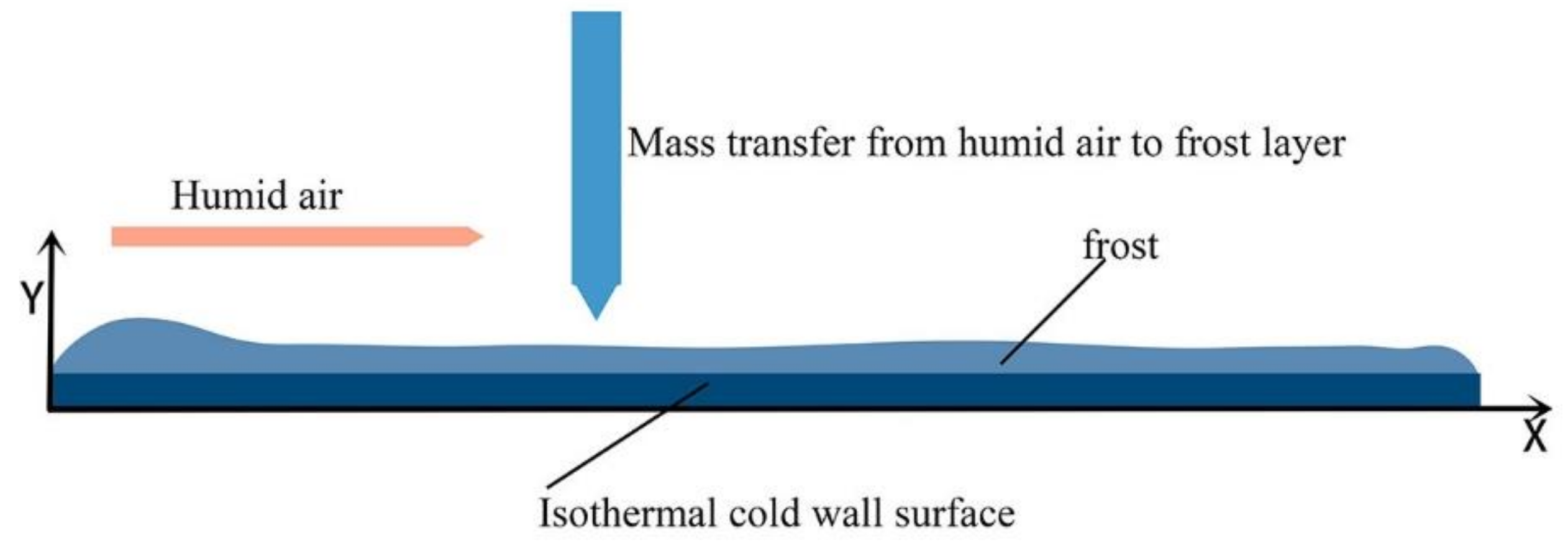
2.1. Frost Growth Mechanism

A schematic diagram to analyze the frosting problem is shown in Figure 1. The substrate is kept at a constant low temperature, and as the wet air flows around the test surface, the water vapor in the wet air undergoes a phase change to form frost, resulting in an increase in the thickness and density of the frost layer.

The frost phase is composed of the wet air and ice phases. The sum of the volume fractions of the ice phase ${\alpha }_i$ and wet air phase ${\alpha }_a$ in each grid is 1.

$${\alpha }_i+{\alpha }_a=1$$

(1)

The frost density can be calculated by the following expression:

$${\rho }_f={\alpha }_i{\rho }_i+{\alpha }_a{\rho }_a$$

(2)

The mass transfer during the frosting process can be divided into two categories. The first category is the mass transfer from water vapor to the frost layer during the whole growth cycle of the frost layer; the second category is the mass transfer from the frost layer to water or water vapor when the surface temperature of the frost layer reaches the freezing point and the melting of the frost layer’s surface occurs. However, because of the complexity of the frost melting process, there is a lack of quantitative studies and corresponding empirical formulas, so the second process is not considered in the frost model of this paper. Since the phenomenon occurs mainly at the stage of full frost growth, the frosting time to be considered in this study is very short, mainly at the initial and growth stages of frosting. Additionally, to simplify the calculation, other assumptions are as follows:

• The wet air is considered to be an incompressible Newtonian fluid with the airflow perpendicular to the inlet direction.
• The airflow and air pressure in the frost layer are uniform, and the airflow at the interface between the wet air and the frost layer is saturated.
• The amount of water vapor absorbed in the control volume during mass transfer in the frost layer is proportional to the density of water vapor in the control volume.
• The gas space in the frost layer is small enough that the natural convection in the frost layer can be neglected, and the heat radiation in the frost layer can be neglected considering the low frost temperature.
• The local humidity of the wet air phase in the control body of the frost layer is consistent with the saturation humidity at that temperature.

The growth of frost density is mainly related to the volume fraction of the second phase in the grid. When the volume fraction of the second phase in the grid exceeds a certain value, it can be considered that frost has formed in the grid. The study of Sungjoon Byun [21] proposed the critical density ${\rho }_{f,c}$, and by determining whether the density in the grid reaches the critical density value, it is possible to determine the intersection of the frost layer and the moist air, and thus the thickness of the frost.

2.2. Mathematical Model

2.2.1. Governing Equations

In this paper, the Eulerian multiphase flow model in Fluent19 is used to simulate multiphase flow in the humid air domain, where the primary phase is wet air and the secondary phase is ice, each phase is represented by a volume fraction $\mathsf{\alpha }$. The governing equations included the mass conservation equations, the momentum conservation equations, the energy conservation equations for each phase, and the species conservation equation for water vapor.

$$\frac{\partial }{\partial t}\left({\alpha }_i{\rho }_i\right)+\nabla \cdot \left({\alpha }_i{\rho }_i{\overrightarrow{u}}_i\right)=S_{mi}$$

(3)

$$\frac{\partial }{\partial t}\left({\alpha }_a{\rho }_a\right)+\nabla \cdot \left({\alpha }_a{\rho }_a{\overrightarrow{u}}_a\right)=S_{ma}$$

(4)

$$\frac{\partial }{\partial t}\left({\alpha }_i{\rho }_i{\overrightarrow{u}}_i\right)+\nabla ·\left({\alpha }_i{\rho }_i{\overrightarrow{u}}_i{\overrightarrow{u}}_i\right)=-{\alpha }_i\nabla p+\nabla ·\stackrel{=}{{\tau }_i}+{\alpha }_i{\rho }_i\overrightarrow{g}+K_{ai}\left({\overrightarrow{u}}_a-{\overrightarrow{u}}_i\right)+S_{ui}$$

(5)

$$\frac{\partial }{\partial t}\left({\alpha }_a{\rho }_a{\overrightarrow{u}}_a\right)+\nabla ·\left({\alpha }_a{\rho }_a{\overrightarrow{u}}_a{\overrightarrow{u}}_a\right)=-{\alpha }_a\nabla p+\nabla ·\stackrel{=}{{\tau }_a}+{\alpha }_a{\rho }_a\overrightarrow{g}+K_{ia}\left({\overrightarrow{u}}_i-{\overrightarrow{u}}_a\right)+S_{ua}$$

(6)

$$\frac{\partial }{\partial t}\left({\alpha }_i{\rho }_i{h}_i\right)+\nabla ·\left({\alpha }_i{\rho }_i{\overrightarrow{u}}_i{h}_i\right)=Q_{ai}-{\alpha }_i\frac{d{p}_i}{dt}+\stackrel{=}{{\tau }_i}:\nabla {\overrightarrow{u}}_i-\nabla ·\overrightarrow{q_i}+S_{hi}$$

(7)

$$\frac{\partial }{\partial t}\left({\alpha }_a{\rho }_a{h}_a\right)+\nabla ·\left({\alpha }_a{\rho }_a{\overrightarrow{u}}_a{h}_a\right)=Q_{ia}-{\alpha }_a\frac{d{p}_a}{dt}+\stackrel{=}{{\tau }_a}:\nabla {\overrightarrow{u}}_a-\nabla ·\overrightarrow{q_a}+S_{ha}$$

(8)

$$\frac{\partial }{\partial t}\left({\alpha }_a{\rho }_a{\omega }_{va}\right)+\nabla ·\left({\alpha }_a{\rho }_a{\omega }_{va}{\overrightarrow{u}}_a\right)=\nabla ·\left({\rho }_a{D}_{h_{2}o}\nabla {\omega }_{va}\right)+S_{va}$$

(9)

The subscripts i and a represent frost layer and wet air respectively. The mass source term is only related to the mass transfer from the water vapor to the ice. The mass source terms are given by:

$$S_{mi}={\dot{m}}_{ai}$$

(10)

$$S_{ma}=-{\dot{m}}_{ai}$$

(11)

$S_{ua}$ is the momentum source term for the humid air phase, and $S_{ui}$ is for the ice phase. The momentum source terms are given by:

$$S_{ui}={\dot{m}}_{ai}{\overrightarrow{u}}_i$$

(12)

$$S_{ua}=-{\dot{m}}_{ai}{\overrightarrow{u}}_a$$

(13)

$S_{ha}$ is the energy source term for the humid air phase, and $S_{hi}$ is for the ice phase. The energy source terms are given by

$$S_{hi}={\dot{m}}_{ai}\left(h_{va}+l_{va}\right)$$

(14)

$$S_{ha}=-{\dot{m}}_{ai}\left(h_{va}\right)$$

(15)

$S_{va}$ is a mass source term for the water vapor component of the humid air:

Where $h_{va}$ is the specific enthalpy of water vapor in wet air, $l_{va}$ is the latent heat of phase change per unit mass of water vapor. The subscript $ai$ indicates the mass transfer from the water vapor component of the wet air to the ice phase.

$S_{va}$ is the mass source term for the water vapor component in the humid air phase and is given by

$$S_{va}=-{\dot{m}}_{ai}$$

(16)

2.2.2. Mass Transfer Rate

According to the frost mathematical model established in the previous literature [21,22,23,24,25,26], each source term in the frost control equation contains the mass transfer rate ${\dot{m}}_{ai}$. Therefore, in order to solve the control equation, the correct mass transfer model is needed: the mass transfer rate from the water vapor in the wet air phase to the ice phase. In this paper, it is considered that the wet air on the surface of the frost layer is in a saturated state and frost occurs when there is a water vapor concentration gradient between the water vapor in the wet air and the water vapor near the cold wall surface. The presence of a water vapor concentration gradient provides the driving force for frost formation. Frost is viewed as a porous structure consisting of wet air and solid ice crystals. After the water vapor in the computational domain forms the ice phase under the frost driving force, the velocity of the ice phase is set to zero, and the fixed ice phase and wet air form the frost structure. With the accumulation of the ice phase and the momentum and heat exchange between the ice phase and the wet air, the simulation of frost growth can be realized.

The driving force for water vapor condensation and freezing is the difference between the partial pressure of water vapor in wet air and the saturation pressure of water vapor corresponding to the frost surface temperature, which is related to the difference in water vapor concentration. The mass transfer rate from wet air to frost is related to the vapor concentration difference and the effective density of wet air [26] (the product of wet air volume fraction and wet air density) with the following mass transfer rate:

$${\dot{m}}_{ai}={\tau }_v·{\alpha }_a·{\rho }_a·\left({\omega }_{va}-{\omega }_s\left(T\right)\right)$$

(17)

Calculation formula of saturated water vapor partial pressure of wet air in reference [27]:

$$p_{vs}=\left\{\begin{array}{c}0.61121\exp \left(\left(18.678-\frac{T}{234.5}\right)\left(\frac{T}{257.14+T}\right)\right),T\ge 0 {}^{{}^{°}}\mathrm{C}\\ 0.61115\exp \left(\left(23.036-\frac{T}{333.7}\right)\left(\frac{T}{279.82+T}\right)\right),T\le 0 {}^{°}\mathrm{C}\end{array}\right.$$

(18)

The saturated water content of the wet air at the corresponding temperature can be obtained from the saturated water vapor partial pressure of the wet air:

$$W_s\left(T\right)=0.622\frac{p_{vs}}{B-p_{vs}}$$

(19)

where B is the atmospheric pressure, B = 101,325 pa, as shown in the Figure, the variation of saturated water vapor partial pressure in wet air with the temperature of wet air (T ≤ 0 °C). As can be seen from Figure 2, the saturated water vapor partial pressure and saturated water content of wet air drop rapidly as the temperature of wet air decreases to about 220 K, and then drops to almost zero.

The mass fraction of water vapor in saturated wet air can be calculated from the saturated humidity content:

$${\omega }_s\left(T\right)=\frac{W_s}{1+W_s}$$

(20)

2.2.3. Conditions for Mass Transfer

Frost deposition and growth in numerical simulations are simulated by setting the velocity of the resulting ice crystal particles to 0. Therefore, a judgment criterion is needed to determine under which conditions the ice phase velocity is set to 0. According to the control equation, the mass conservation equation of the ice phase is as follows:

$$\frac{\partial }{\partial t}\left({\alpha }_i{\rho }_i\right)+\nabla \cdot \left({\alpha }_i{\rho }_i{\overrightarrow{u}}_i\right)=S_{mi}$$

(21)

$S_{mi}$ ($kg/\left(m^3·s\right)$) is the mass source term caused by phase transition. In the numerical model of this study, all substances are considered fluids, so each phase has a convective term. In the actual frost formation process, the ice phase that constitutes the frost does not move, so the convective term in the above equation (the second phase at the left end of the equation) can be neglected and the equation can be simplified to:

$$\frac{\partial }{\partial t}\left({\alpha }_i{\rho }_i\right)=S_{mi}$$

(22)

In the calculation, considering the assumption that the density of the ice phase is constant, the above equation can be further expressed as:

$$\frac{\partial {\alpha }_i}{\partial t}=S_{mi}/{\rho }_i$$

(23)

The above equation can be viewed as the rate of change of the volume fraction of the ice phase. The critical frost density is the minimum density that frost must exceed, and is an important reference value for judging frost. In the numerical calculations of this paper, the formula for the critical density in the literature [21] is referenced. In the study of the literature [21], the trial and error method was used to calculate the best predicted critical density of frost thickness and frost density under various operating conditions, and the empirical formula of critical frost density value was obtained by regression analysis:

$${\rho }_{f,c}={\rho }_{ice}\left(0.533{\left(2+\frac{T_w}{273.15}\right)}^{\frac{1}{6}}{\left(2+\frac{T_{a,in}}{273.15}\right)}^{\frac{1}{3}}-0.698\right)$$

(24)

where ${\rho }_{ice},T_w, T_{a,in}$ are ice density, cooling surface temperature, and inlet wet air temperature, respectively, and $-160 {}^{°}\mathrm{C}\le T_w\le -100 {}^{°}\mathrm{C}\le$  $10 {}^{°}\mathrm{C}\le T_{a,in}\le 25 {}^{°}\mathrm{C}$. The results of empirical equations show that cold surface temperature and air temperature are the main influencing factors of critical frost layer density. The derivation of wall surface temperature and wet air temperature in the expression of critical frost layer density are obtained separately:

$${\rho }_{f,c}{}_{Tw}^{,}={\rho }_{ice}\left(0.000325*{\left(2+\frac{T_w}{273.15}\right)}^{-\frac{5}{6}}{\left(2+\frac{T_{a,in}}{273.15}\right)}^{\frac{1}{3}}\right)$$

(25)

$${\rho }_{f,c}{}_{Ta,in}^{,}={\rho }_{ice}(0.00065*{\left(2+\frac{T_w}{273.15}\right)}^{\frac{1}{6}}{\left(2+\frac{T_{a,in}}{273.15}\right)}^{-\frac{1}{3}}$$

(26)

From the expressions (25) and (26), it can be concluded that:${\rho }_{f,c}{}_{Tw}^{,}>0,{\rho }_{f,c}{}_{Ta,in}^{,}>0$. In the applicable temperature range of critical density, the critical density of frost layer increases with the increase of wall temperature and inlet wet air temperature.

In the operating temperature range of the pre-cooler, the following equation has been used in the numerical calculation model for frosting that has been developed in this study as a criterion for determining frosting:

$$\left\{\begin{array}{c}\frac{\partial {\alpha }_i}{\partial t}=S_{mi}/{\rho }_i\\ {\rho }_{f,\mathrm{c}}\end{array}\right.$$

(27)

The frost density obtained by numerical calculation is given by the equation: ${\rho }_{f,avg}={\alpha }_i{\rho }_i+\left(1-{\alpha }_i\right){\rho }_{air}$, where $\left(1-{\alpha }_i\right)$ is a value less than 1 and decreases as the frost density increases. The analysis shows that the dominant term of the frost density is ${\alpha }_i{\rho }_i$. When the frost reaches the critical frost density, it can be approximated as:${\alpha }_{i,c}{\rho }_i={\rho }_{f,c}$. From the above equation, the minimum volume fraction of the ice phase in the frost layer formed after the entire calculation time t can be obtained:

$${\alpha }_{i,c}={\rho }_{f,c}/{\rho }_i$$

(28)

According to the existing literature on frost density, the variation of frost density at different frost growth stages during the frosting process is not uniform. According to ${\alpha }_{i,c}$ and numerical calculation time T, the reference value of the rate of change of ${\alpha }_i$ can be obtained: ${\alpha }_i=\frac{S_{mi}}{{\rho }_i}>\epsilon$, which is used as the criterion for judging the frost formation under the working conditions (super low temperature) of the pre-cooler.

2.2.4. Boundary conditions

$\mathrm{Velocity} \mathrm{inlet}$:

$$u_a=u_{in}, v_a=0, w_a=0, T_a=T_{in}, {\omega }_v={\omega }_{in}$$

(29)

$$u_i=0,\hspace{1em}{v}_i=0,\hspace{1em}{w}_i=0,\hspace{1em}{T}_i=T_{in},\hspace{1em}{\alpha }_i=0$$

(30)

Out flow:

$$\frac{\partial u_a}{\partial n}=0, \frac{\partial v_a}{\partial n}=0,\frac{\partial w_a}{\partial n}=0,\frac{\partial T_a}{\partial n}=0,\frac{\partial {\omega }_v}{\partial n}=0$$

(31)

$$\frac{\partial u_i}{\partial n}=0, \frac{\partial v_i}{\partial n}=0,\frac{\partial w_i}{\partial n}=0,\frac{\partial T_i}{\partial n}=0,\frac{\partial {\alpha }_i}{\partial n}=0$$

(32)

Constant temperature wall:

$$u_a=0, v_a=0, w_a=0, T_a=T_w, \frac{\partial {\omega }_v}{\partial n}=0$$

(33)

$$u_a=0, v_i=0, w_i=0, T_i=T_w, \frac{\partial {\alpha }_i}{\partial n}=0$$

(34)

Symmetry surfaces:

$$\frac{\partial u_a}{\partial n}=0, \frac{\partial v_a}{\partial n}=0,w_a=0,\frac{\partial T_a}{\partial n}=0,\frac{\partial {\omega }_v}{\partial n}=0$$

(35)

$$\frac{\partial u_i}{\partial n}=0, \frac{\partial v_i}{\partial n}=0,w_i=0,\frac{\partial T_i}{\partial n}=0,\frac{\partial {\alpha }_i}{\partial n}=0$$

(36)

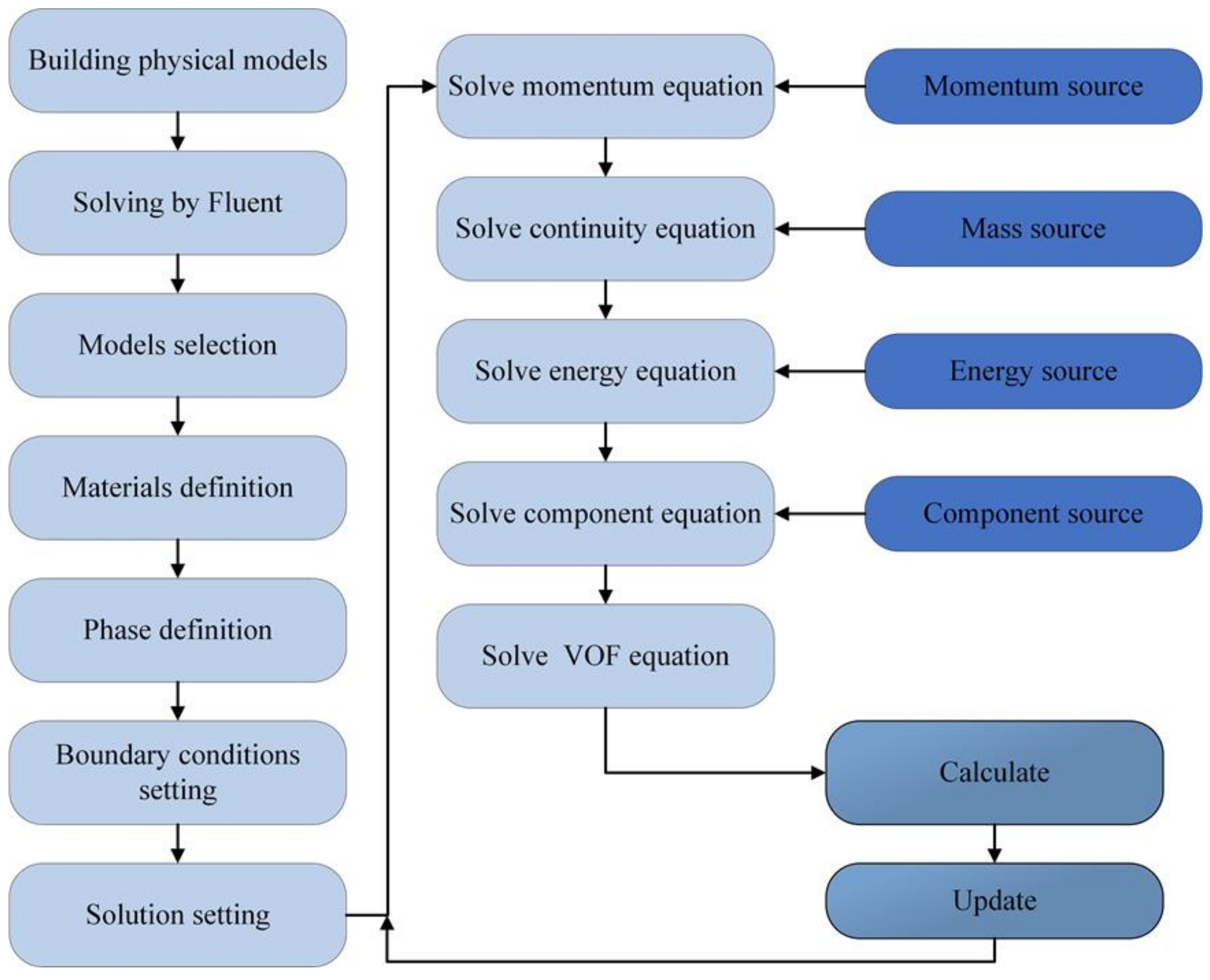
2.3. Solution Scheme

A detailed simulation flow is shown in Figure 3. There are two phases in the computing domain. The first phase is moist air containing water vapor and dry air. The moist air is treated as a mixture and the thermal conductivity is taken as the value of dry air and the density-specific heat and viscosity are calculated as weighted averages. The secondary phase is ice, and the particle diameter of the ice crystals was set to ${10}^{-5}$ m.

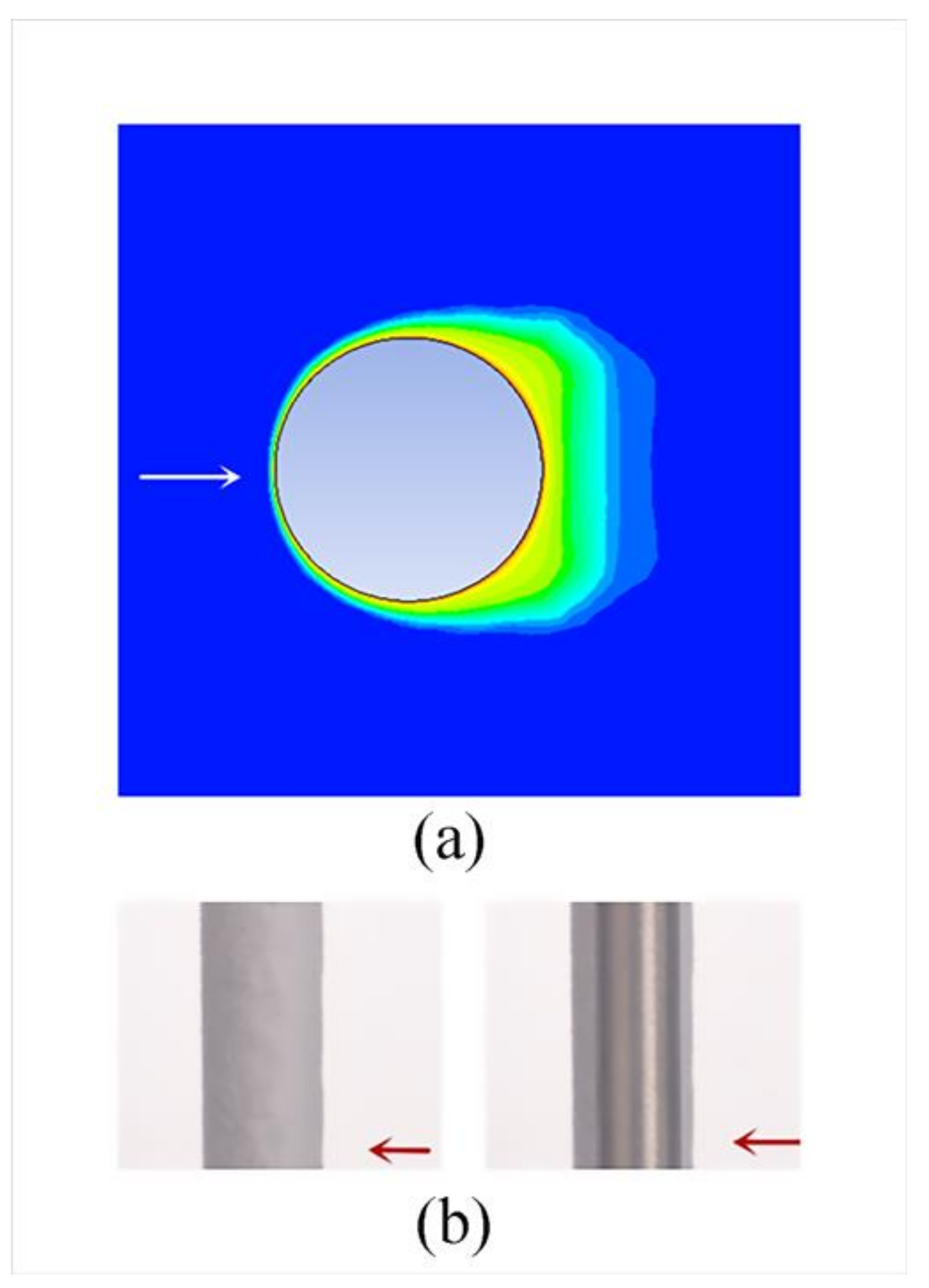
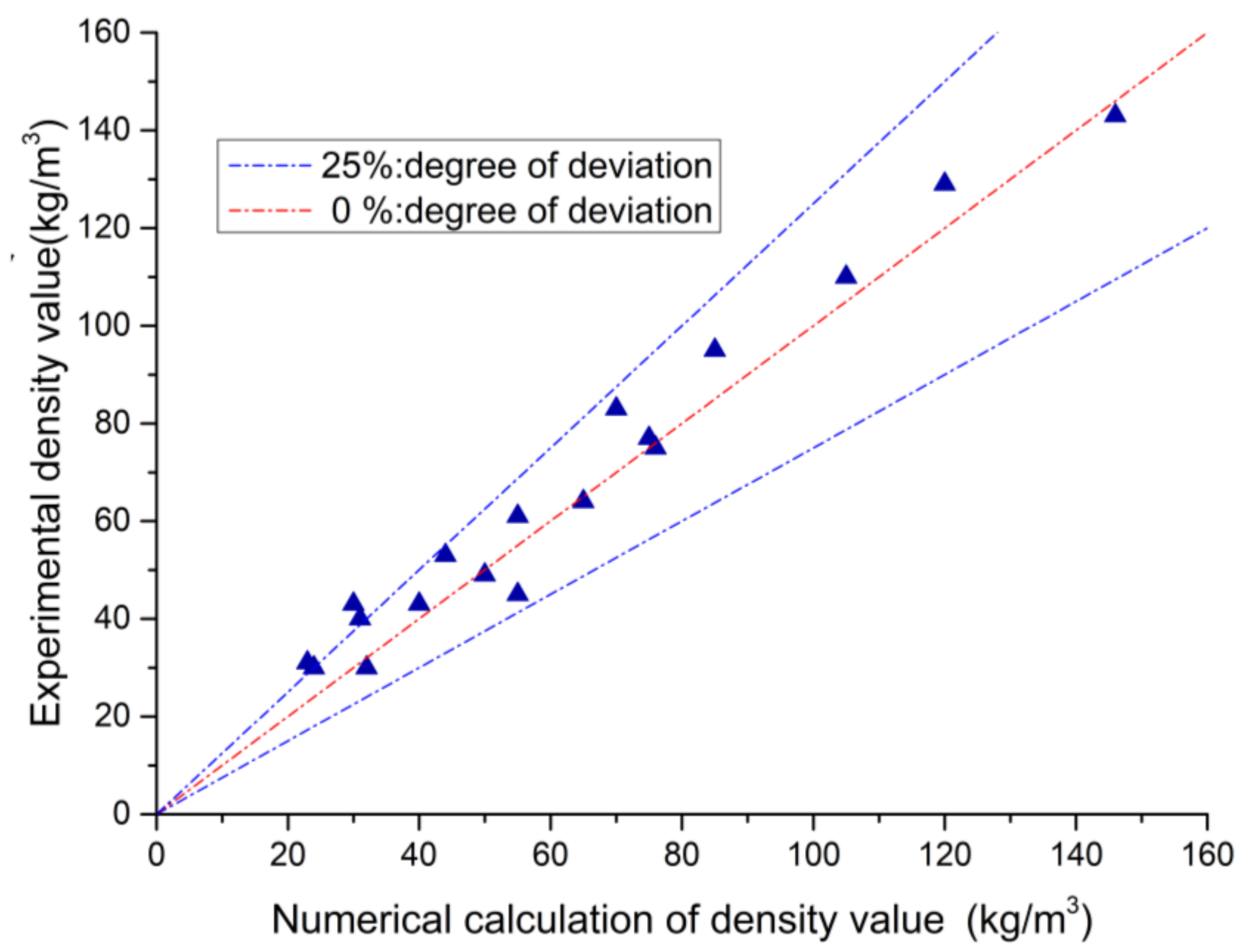
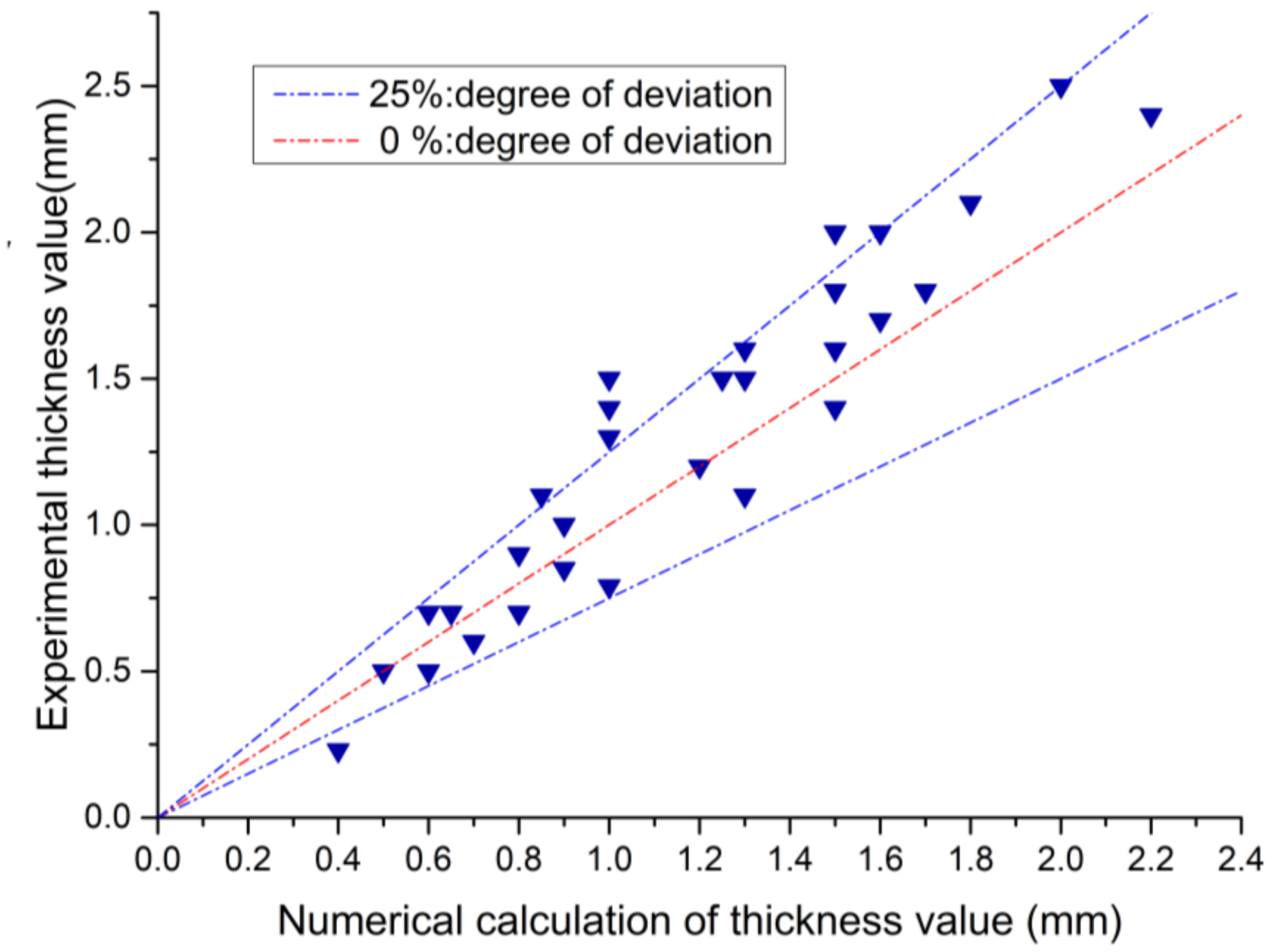
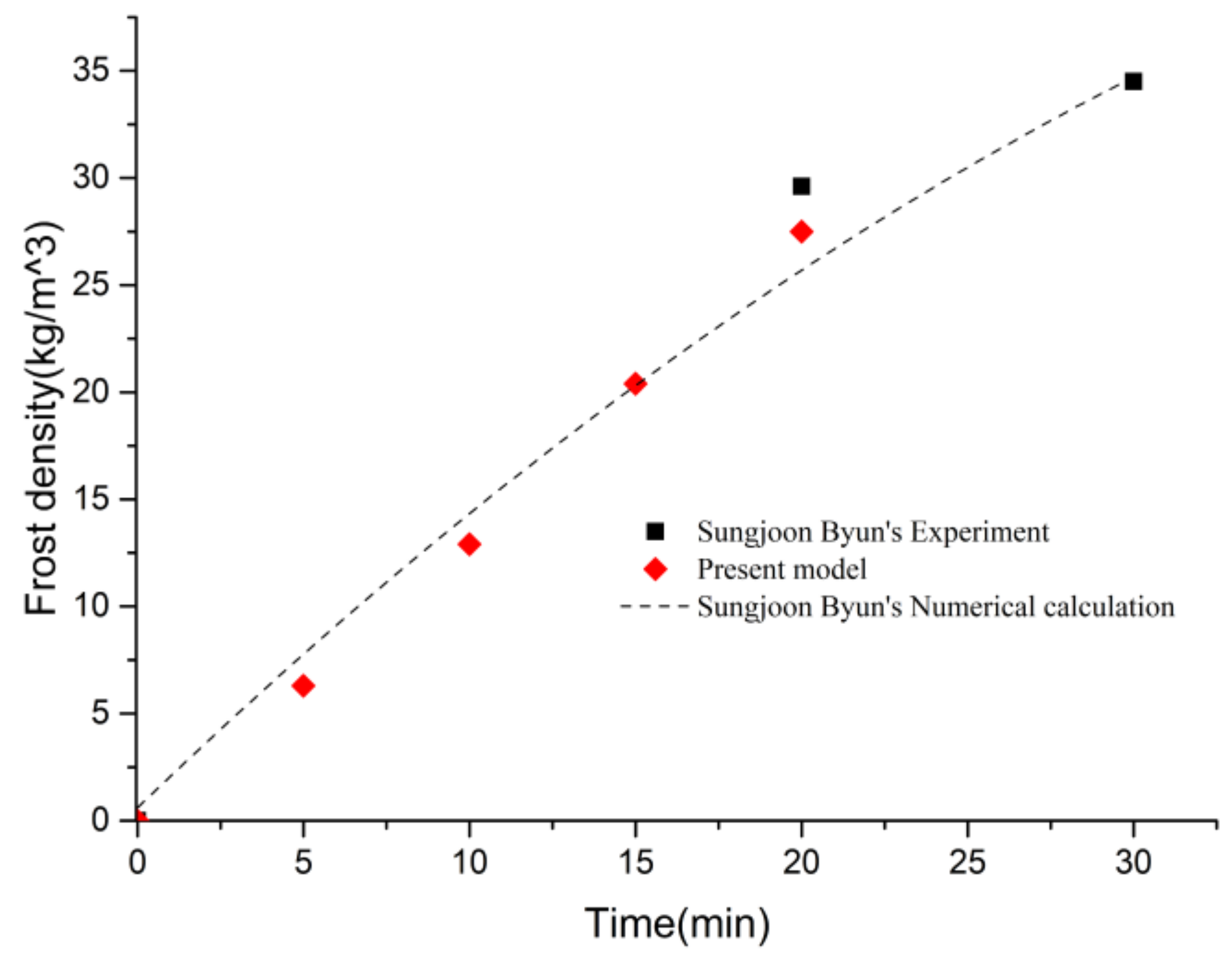
2.4. Model Verification

The proposed numerical model of frosting was used to calculate frosting under the experimental conditions in references [21,28,29,30], and each experimental condition is shown in

Table 1. Flat plate frosting calculation parameters.

Number	$\mathbf{Humid} \mathbf{Air} \mathbf{Temperature} ({\mathit{T}}_{\mathit{a}\mathit{i}\mathit{r}}$$/{}^{°}\mathrm{C})$	Relative Humidity	$\mathbf{Cold} \mathbf{Wall} \mathbf{Surface} \mathbf{Temperature} ({}^{°}\mathrm{C})$	$\mathbf{Humid} \mathbf{Air} \mathbf{Flow} \mathbf{Rate} \left(\mathbf{m}/\mathbf{s}\right)$
1	10.5	80%	−8	5
2	22	80%	−15	0.7
3	15	68%	−130	2
4	15	48.7%	−130	1.5
5	10	29.2%	−160	1
6	20	67.8%	−100	2
7	10.5	80%	−10.5	5
8	16	80%	−16	0.7

. The frost thickness and frost density were also compared to verify the correctness of the frost model. The physical model of frosting used is a wet air cross-swept cooling plate, which is simulated as a simplified two-dimensional model. Due to the simplicity of the plate model, the frost criterion is mainly considered in the validation calculation of the plate with the flow rate and temperature of the wet air, and the validation results are shown in Figure 4 and Figure 5. The abscissa of the triangle in Figure 4 and Figure 5 represents the results obtained from the model in this paper, and the ordinate represents the experimental results from the references [21,28,29,30].The dashed lines in Figure 4 and Figure 5 represent the degree of deviation of the numerical calculation results from the experimental results.

For the wall temperature conditions within the working range of the pre-cooler, the frost criterion proposed in the previous section is applied to the frost calculation under single tube forced convection, and the calculated frost density is compared with the density obtained from the forced convection frost experiment on the ultra-low temperature surface in the Sungjoon Byun’s literature [21], as shown in Figure 6. Additionally, the frost pattern obtained from the numerical calculation of a single tube matches the experimentally obtained frost pattern in the literature [31], as shown in Figure 7.

3. Simulation Experiment

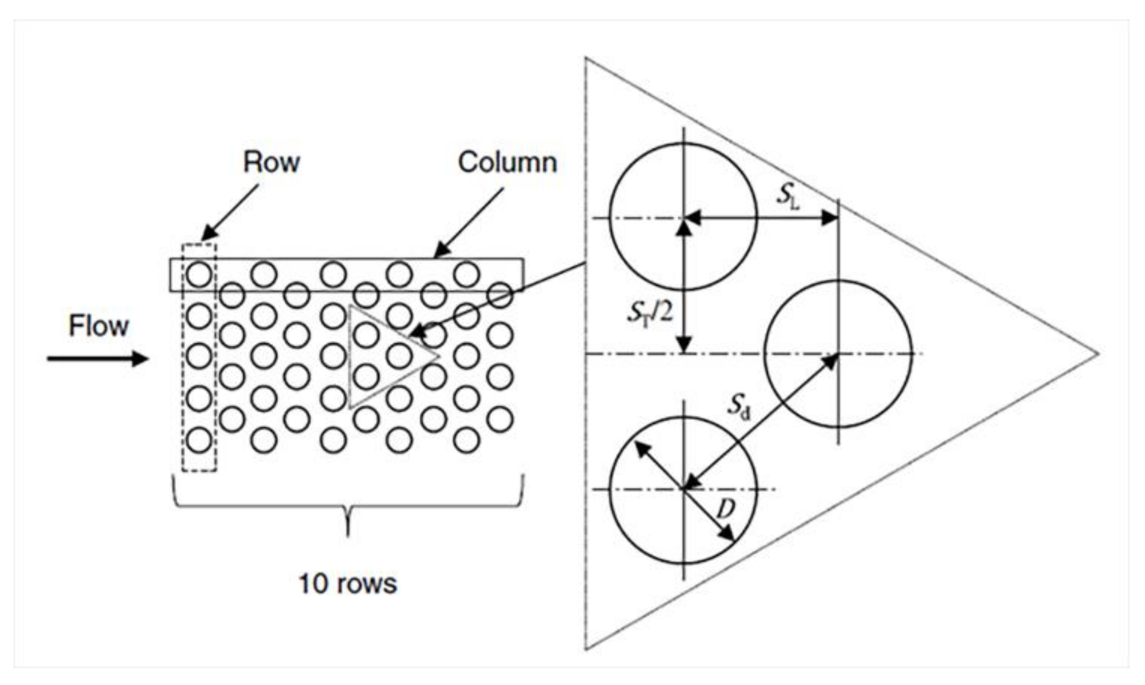
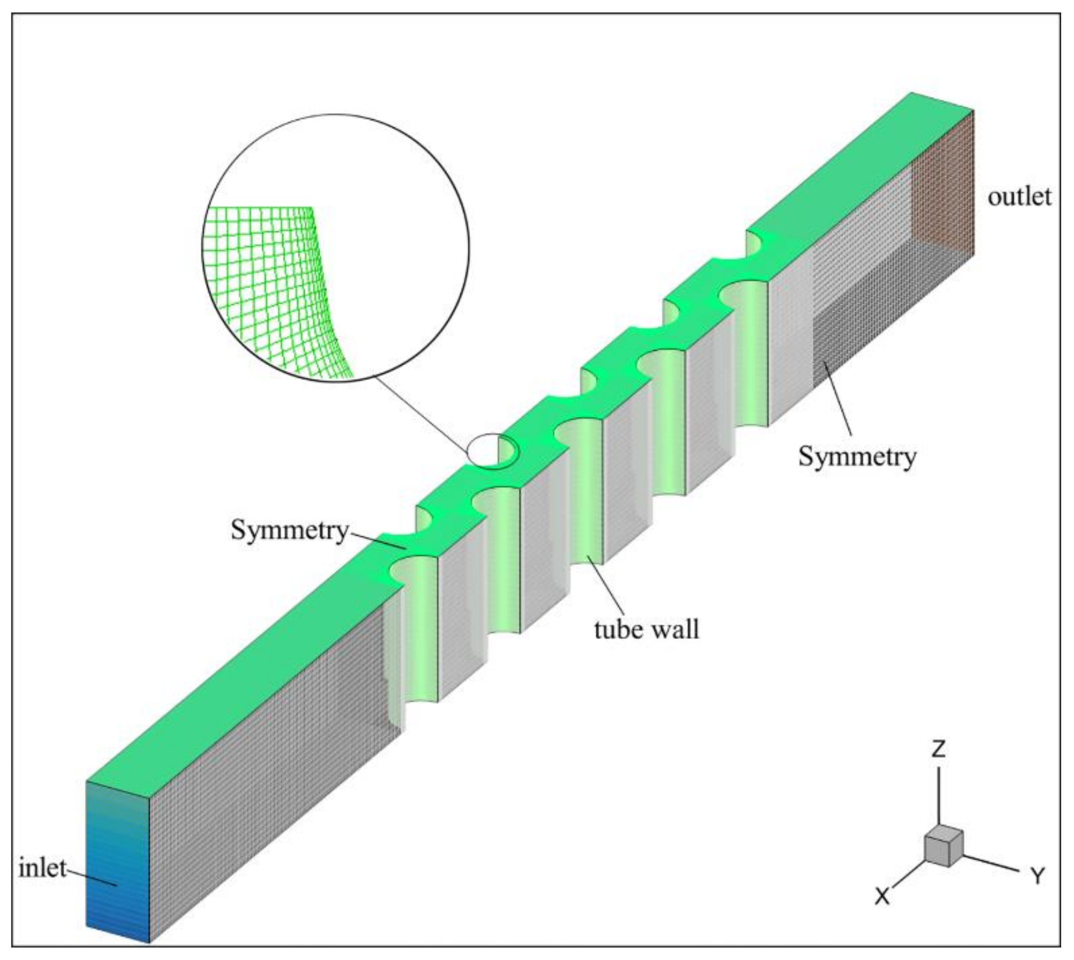
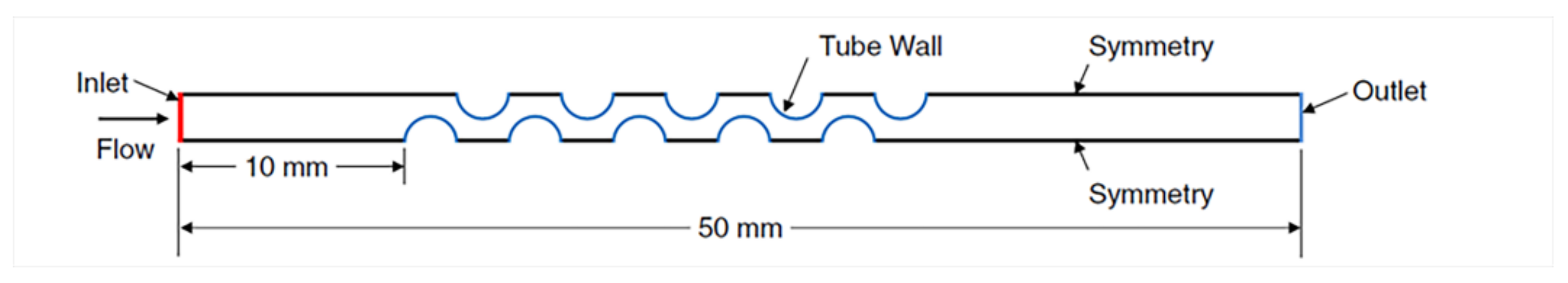
3.1. Physical Model

It is shown that the ratio of the diameter of the entire pre-cooling module to the diameter of the circular tube used in the pre-cooler tube set is ${10}^{-3}$, so the effect of the curvature of the circular tube on the flow field can be ignored [32]. In the process of building the calculation model, the curvature of the circular tube can be simplified to a straight tube without considering the curvature of the circular tube. According to Rukausska’s research on cross-swept tube bundles [33], the resistance to flow during heat exchange between fluid and cross-row tube bundles depends on the flow characteristics of the fluid in the bundle. Rukausska proved experimentally that when the number of tube rows is small, the resistance of the front row of round tubes will be different from the average resistance of the bundle, while when the number of rows is greater than nine, the resistance coefficients of each row of the bundle are equal. The structure diagram of the transverse tube group used by the Reaction Engines Ltd (Culham Science Centre, Abingdon OX14 3DB, UK). [34] is shown in Figure 8. From the diagram, it can be seen that the horizontal spacing $S_T$ and the longitudinal spacing $S_L$ determine the arrangement of the tube bundle. For the circular tube group arrangement, the pitch ratios $p_L$ and $p_T$ are defined as follows:

$$p_L=\frac{S_L}{D}$$

(37)

$$p_T=\frac{S_T}{D}$$

(38)

The $p_L$ and $p_T$ used in the SABER precooler study were 1.25 and 2.2, respectively, on the basis of which the computational model for a tube bundle of 2 mm diameter was developed. The Figure 9 [31] shows the entire calculation area and boundary conditions, which includes an upstream auxiliary area 10 mm in length and a downstream area of the same length. The total length of the calculation area is set to 50 mm and the number of rows of tubes is taken as 10. The divided mesh is shown in Figure 10 and the mesh is densified near all tube walls. In order to reduce the number of meshes and increase the computational speed, the thickness in the Z-direction is taken as 5 mm and a symmetric boundary condition is used between the half-tubes to simulate the flow between the row of tube bundles in the actual pre-cooler model.

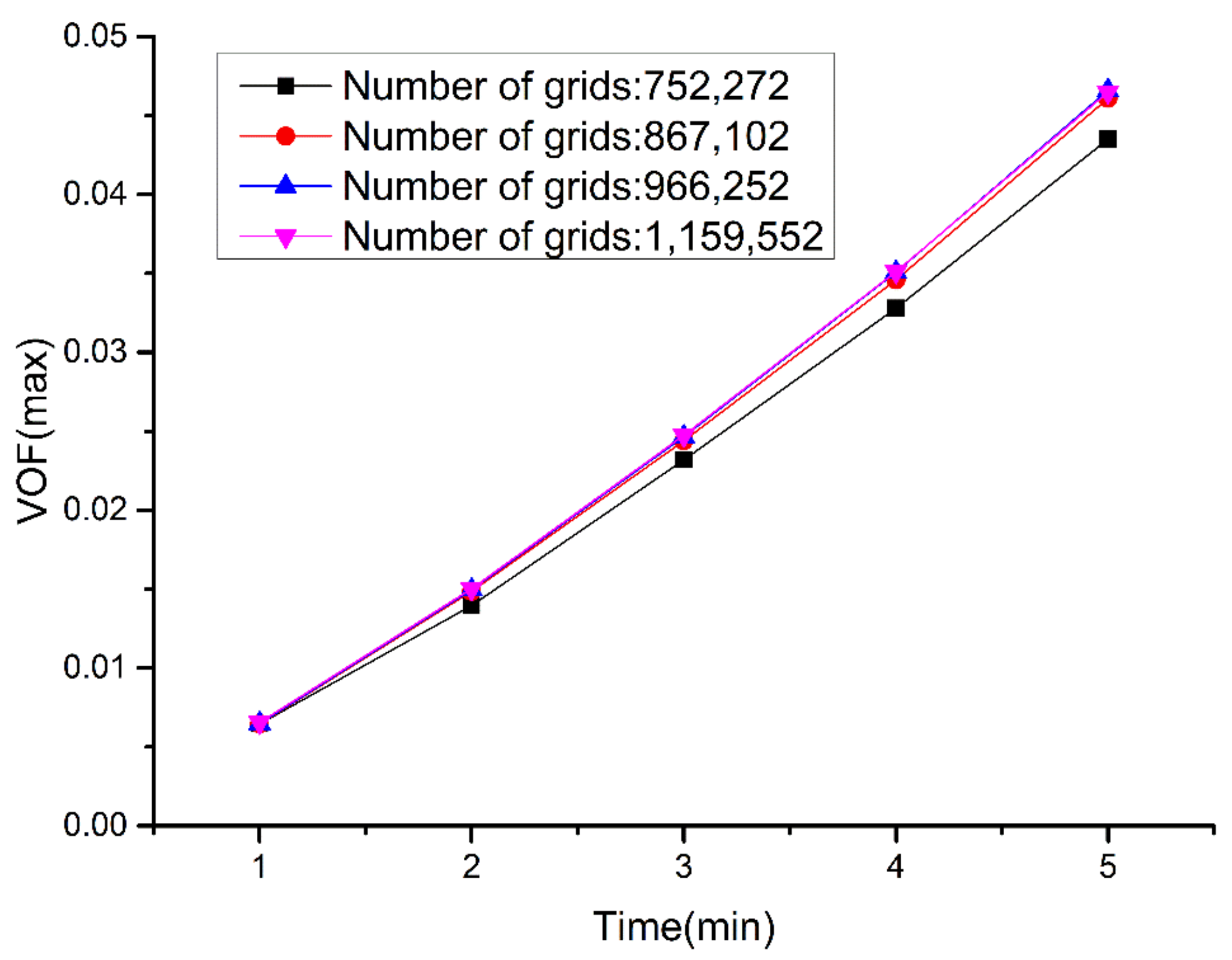
3.2. Grid-Independent Analysis

According to the established calculation model, the grid is divided and the grid near the pipe wall is encrypted to ensure the stability and accuracy of the calculation. The total number of grids in the four groups is 752,272, 867,102, 966,252, and 1,159,522. For different grids, the variations of the maximum volume fraction of the ice phase ($VO{F}_{ice-max}$) at a total duration of 5 min were calculated at a water vapor content of 6.4 g/kg (RH = 38%), an airflow velocity of 12 m/s, an inlet wet air temperature of $t_{in}$= 1000 K, and a tube wall temperature of 160 K. The calculation results are shown in Figure 11.

When the total number of grids is 752,272, the maximum error in the calculated ice phase volume fraction is relatively large, with a maximum error of ε = 5%. The maximum errors for 867,102, 966,252 and 1,159,522 grids were ε = 1%, ε = 2%, and ε = 2.1%, but the calculation time was significantly higher when the number of grids was 1,159,552. Considering the accuracy and computational efficiency, we choose 867,102 grids for subsequent calculations.

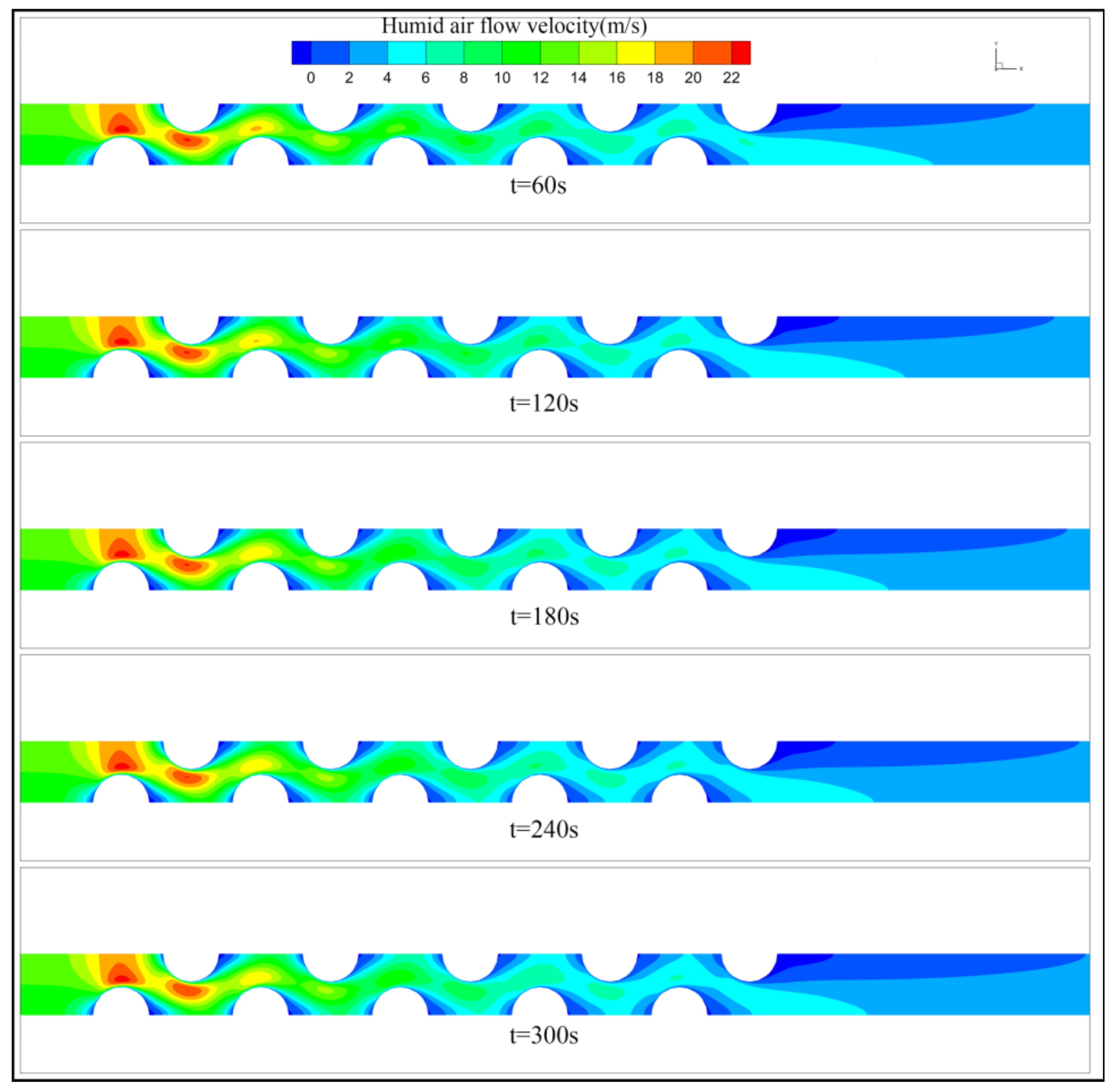
3.3. Numerical Calculation of Tube Bundle Frosting

During the heat exchange between the tube bundle and the wet air, the temperature of the wet air will decrease continuously along the flow direction, and the frosting on the circular tubes at different locations will be significantly different. In this section, the tube bundle frosting will be investigated based on the numerical calculation of single tube frosting. According to the ground test of the pre-cooler, the inlet airflow temperature is set to 1473 k, and the value ranges of other parameters are shown in

Table 2. Numerical calculation parameters for tube bundle frosting.

Wall Temperature (K)	Water Vapor Content (g/kg)	Inlet Flow Rate (m/s)
120–180	6.08–7.43	8–20

. For tube bundle structure a characteristic flow velocity is needed to calculate the Reynolds number, which is generally taken as the maximum flow velocity in the tube bundle. For a given range of inlet flow velocities, the maximum flow velocity between the bundles ranges from 14–38 m/s. The Reynolds number is calculated in the range of 300–800 for the calculated conditions. The turbulence model for numerical calculations in this paper uses the $Standard k-\epsilon$ model in Fluent19.

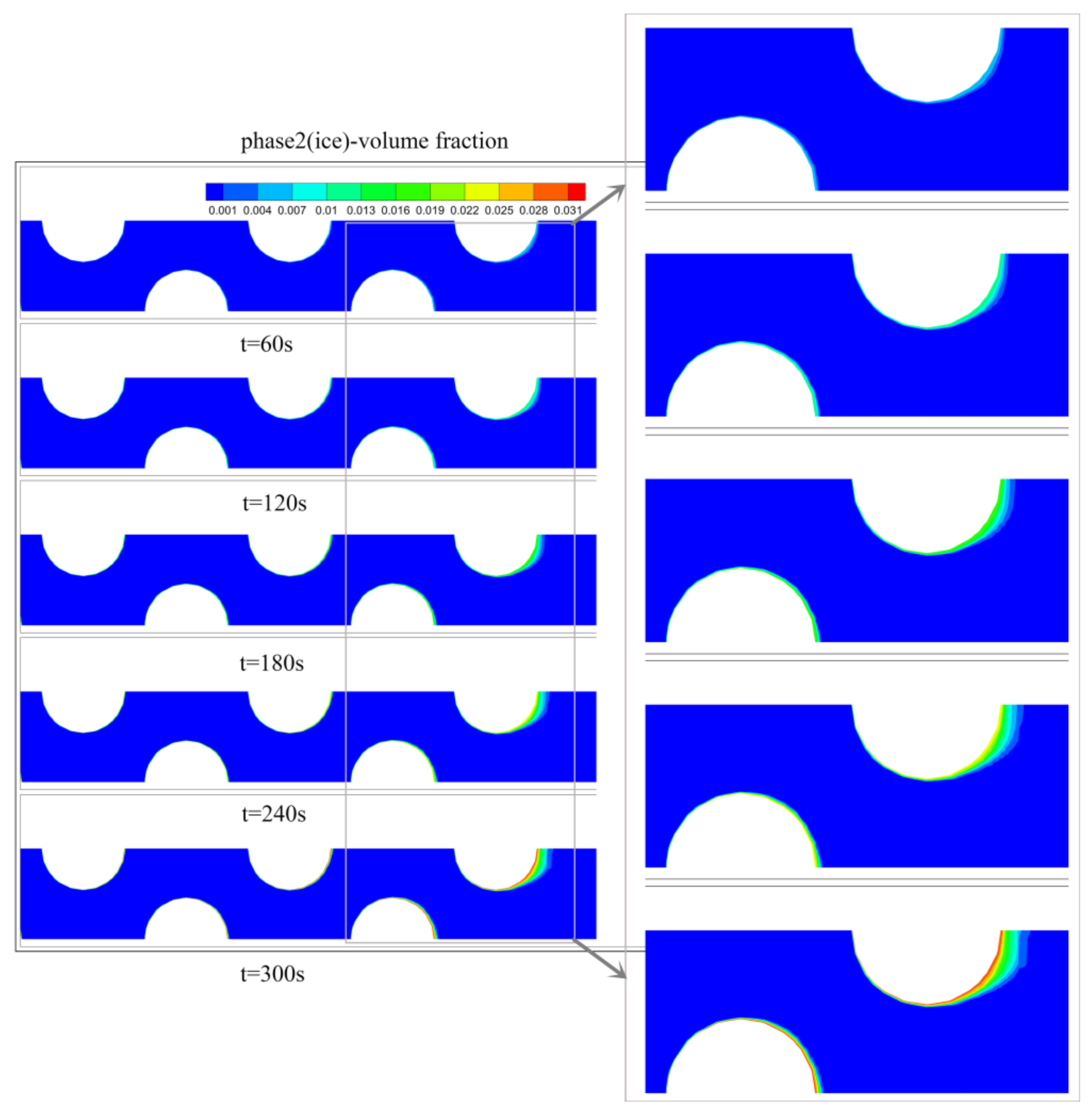
3.3.1. Distribution of Frost on Tube Bundle

As shown in Figure 12, the inlet wet air temperature is 1473 k, the tube wall temperature is 180 K, the inlet flow rate is u = 12 m/s, the moisture content of wet air ${\omega }_{in}=6.4 \mathrm{g}/\mathrm{kg}$, and the frost distribution on the tube bundle after frosting for 5 min.

From Figure 12, it can be seen that there are significant differences in the frosting on the tube wall at different locations. In the calculated time duration, the frost layer formed on the first seven rows of round tubes in the tube bundle is thin, and there is no obvious thickness increase throughout the calculated time duration, while the frost layer in the 8th to 10th rows of the tube bundle has an obvious thickening and density growth process. Frosting occurs at locations where the wet air temperature is below the freezing point and meets the frosting criteria. The wet air temperature around the front of the circular tube is relatively high, and frost only occurs in the thinner part of the wet air temperature boundary layer at the front of the circular tube. The heat flux and temperature gradient between the wet air and the circular tube are relatively large. When the wet air flows through the rear tube bundle, the temperature of the wet air drops significantly, the temperature gradient between the wet air and the tube wall is small, and the area meeting the frost conditions is large. As a result, a frost layer with a certain thickness is formed around the rear circular tube, and the frost layer becomes thicker and more dense as time passes. According to the velocity distribution around each circular tube before and after frosting, the low-velocity area on the backwind side of the tube bundle gradually increases with the growth of the frost layer, which is favorable to the growth of the frost layer. As shown in Figure 13, the velocity field of the wet air around the tube bundle varies with frosting. It can be seen that the velocity field of the wet air around the round tubes near the front row does not change much as the frosting proceeds, while the low-velocity area of the wet air on the back side of the round tubes increases around the tube bundles in the back row as the frost layer grows.

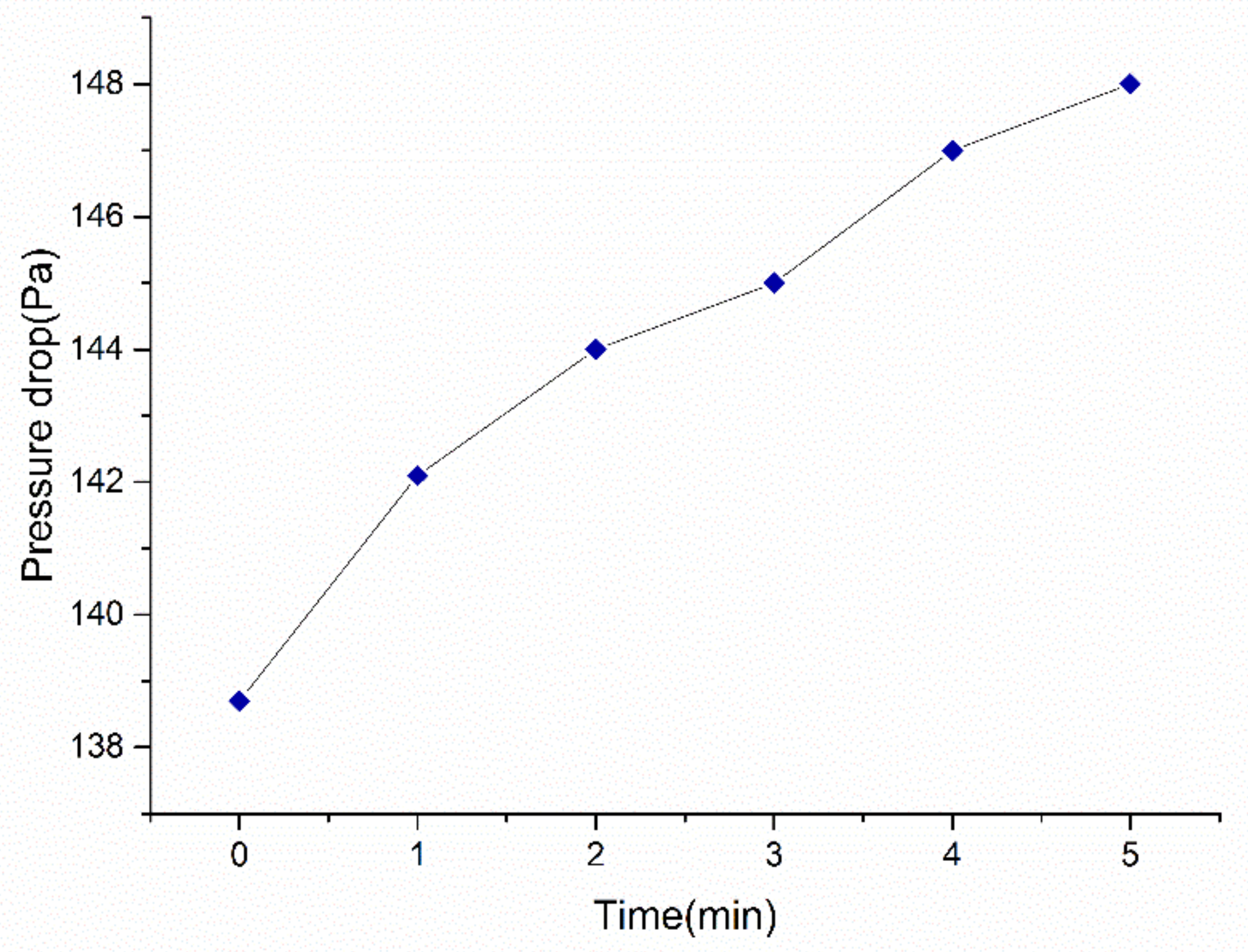
3.3.2. Humid Air Pressure Drop

As the frost layer thickens and grows and densifies, the frost layer will continue to occupy the passage of wet air, which in turn affects the velocity field of wet air, and the pressure drop of wet air will continue to increase, as shown in Figure 14. As can be seen in Figure 14, the pressure drops at minute 5 increased by 6.7% compared to minute 0. The frost layer growth influences the wet airflow velocity distribution in the calculation domain while the influence on the pressure drop after the wet air flows through the frosted tube bundle is not negligible. The effect of the change in the growth rate of the frost layer on the pressure drop of the wet air is significant, and this will be continued in the subsequent sections.

4. Frosting under Different Influence Factors

4.1. Frosting at Different Refrigerant Temperatures

In the actual operation of the pre-cooler, the cooling effect on the wet air differs due to the different cooling media in the tubes. Different tube wall temperatures are used to calculate the difference in the frost morphology of the tube bundle. As shown in the Figure, the frost clouds at 3 min on the circular tubes in rows 6–10 in the tube bundle when the tube wall temperature is $T_w$= 165 K, 175 K, and 180 K, respectively.

In the actual operation of the pre-cooler, the cooling effect on the wet air varies due to the different cooling media in the tubes. It is necessary to carry out the effect of different refrigerant temperatures on the frosting of the tube bundle. The differences in the frost morphology obtained by numerical calculations at different tube wall temperatures are shown in the figure (tube wall temperatures are $T_w$= 165 K, 175 K, and 180 K, respectively). Figure 15 shows the cloud at 3 min of frosting on the circular tubes in rows 6–10 of the tube bundle.

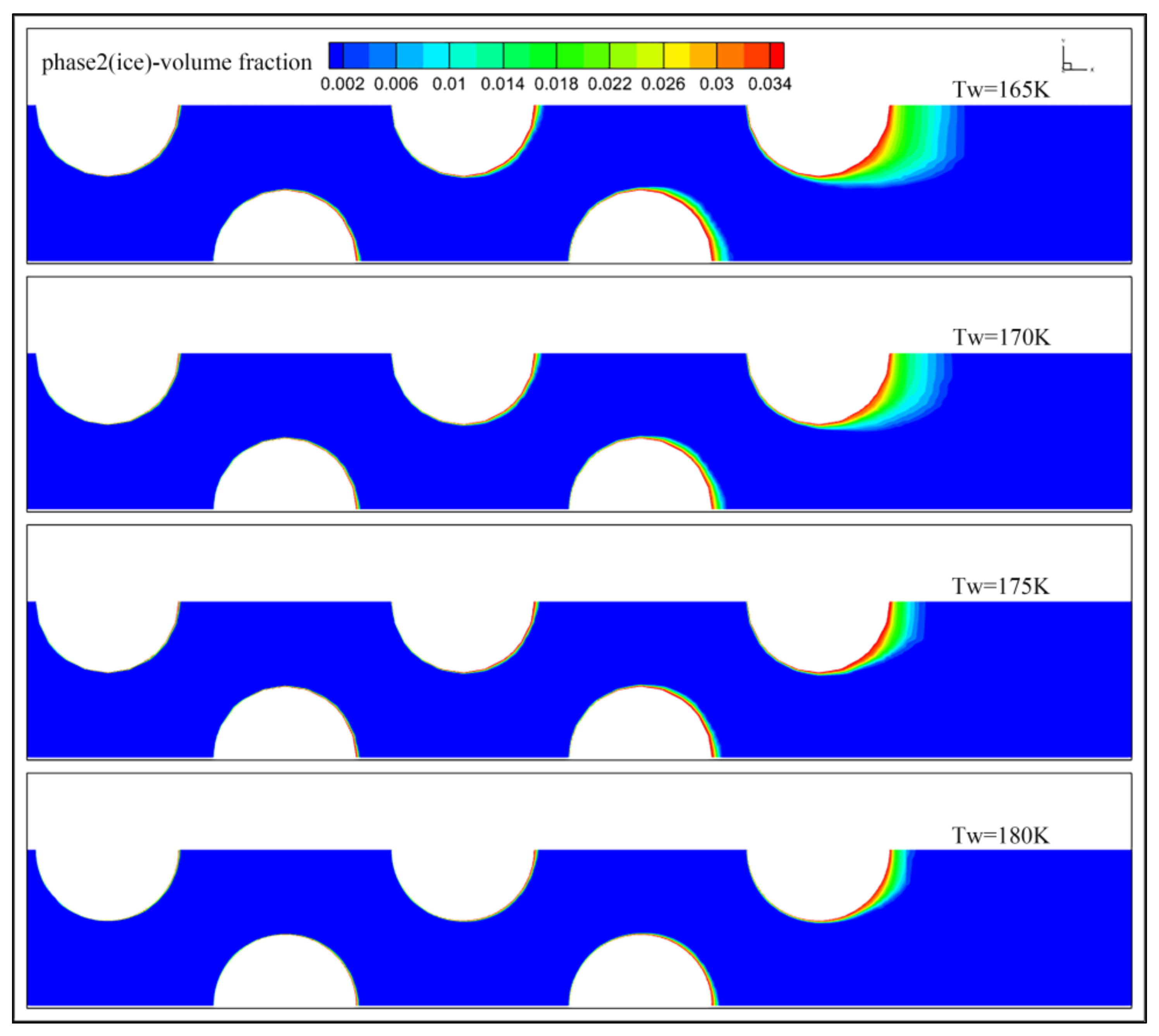
4.1.1. Frost Layer Morphology at Different Refrigerant Temperatures

(1)

The overall frost layer formed on each round tube at the beginning of frosting is very thin and the frost density is very low for different wall temperature conditions. At the beginning of frosting, the thickness of the frost layer formed on the wall of the back row (rows 8 to 10) is relatively thick compared to the front row (rows 1 to 7). At different wall temperatures, the thickness of the frost layer formed on rows 8 to 10 at the same time varied significantly. Additionally, the lower the wall temperature, the thicker the frost layer formed on the wall of the 10th row under the same conditions of other parameters. For example, the thickness of the frost layer formed at a wall temperature of 165 K in the 5th minute is about 3 times thicker than that at 180 K. It can be assumed that the frost layer growth is very sensitive to the change of the tube wall temperature. The maximum volume fraction of the second phase (ice phase) formed under the four wall temperature conditions is in the same order of magnitude, while the thickness of the frost layer is significantly different for the same calculation duration, indicating that the effect of the wall temperature on the frost layer growth rate is very obvious. Combined with the mass transfer rate equation:${\dot{m}}_{ai}={\tau }_v·{\alpha }_a·{\rho }_a·\left({\omega }_{va}-{\omega }_s\left(T\right)\right)$, it can be inferred that the lower the wall temperature the higher the frost driving force and the higher the mass transfer rate.

(2)

The growth morphology of the frost on the tube bundle is similar to the numerical calculation of the frost on a single tube. The volume fraction distribution of the second phase on the same tube wall can reflect the mass transfer capacity at different locations on the tube wall. As the high-temperature wet air flows through the tube bundle, the heat exchange between the wet air and the tube bundle is accompanied by a mass transfer from water vapor to frost. In the mass transfer process from water vapor to ice in the phase change process there is also the release of latent heat of phase change. The latent heat will affect the temperature distribution of wet air around the tube wall together with the wall temperature, resulting in differences in the thickness and density of the frost layer at different locations on the same tube wall. The wet air temperature gradually decreases along the flow direction, while the velocity of the wet air is constantly changing, and the heat transfer capacity of the wet air and the tube bundle at different locations is also changing. Therefore, it causes the difference in frost layer density on the circular tube at different locations.

(3)

The thickness of the frost layer formed on the wall of each tube increases with time. However, the increase in the thickness of the frost layer on the wall of the front row of tubes was not significant and the change in thickness was almost negligible. This is mainly due to the high inlet wet air temperature, which is taken as 1473 K. Although the wall temperature is ultra-low temperature, the temperature around the front wall is still high and the mass transfer coefficient is very low, and the frost layer can be formed very thin, and the frost layer has almost no effect on the surrounding temperature distribution. Therefore, no significant frost layer growth could be observed on the front row of round tubes.

(4)

The morphology of the frost layer formed on the tube bundle is slightly different from that calculated for single-tube frosting, as can be seen from the morphology of the frost layer in rows 9 and 10. One of the dominant factors affecting the formation of the frost layer is the temperature of the moist air. The wet air flowing in the tube bundle is jointly influenced by the adjacent circular tubes and the temperature field is different from that around the single circular tube, so the shape of the frost layer on the tube bundle is also different from that of the single tube.

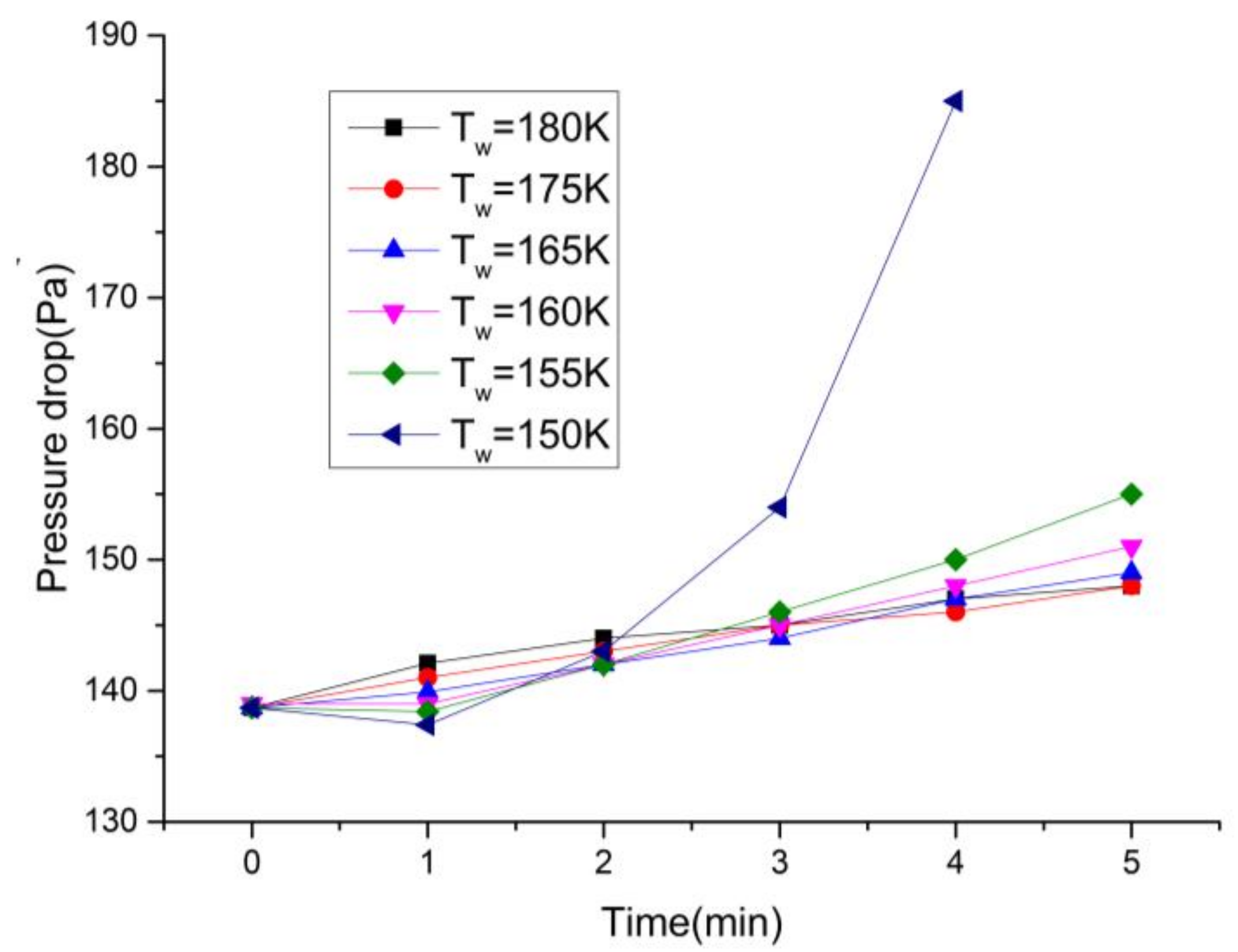
4.1.2. Pressure Drop at Different Refrigerant Temperatures

As shown in Figure 16, the variation of inlet and outlet pressure drop after frosting of wet air at different wall temperatures. From the figure, it can be seen that the pressure drop at the beginning of frosting (1 min) does not vary much at different wall temperatures. As the frosting proceeds, the pressure drop after the wet air flows through the tube bundle increases continuously, and the difference is gradually obvious at different wall temperatures. According to the frost cloud diagram, the thickness of the frost layer formed on the inner wall of the tube is very similar at 180 K and 175 K. Therefore, there is almost no difference in the pressure drop caused by the two wall temperature conditions during the whole calculation time. From the previous analysis, it is clear that the effect on the mass transfer coefficient increases continuously as the tube wall temperature decreases. The growth rate of the frost layer on the tube wall and the difference in the frost morphology increase, so the pressure drop also increases with the formation of frost. The pressure drop at the 5th minute at 155 K wall temperature increases by 16.2% compared to 180 K. The pressure drop at the 5th minute at 150 K wall temperature increases by 16.2% compared to 180 K. The pressure drop at the 4th minute at 150 K wall temperature increased by 25% compared to 180 K. This indicates that the wall temperature affects the pressure drop after frosting and indirectly affects the pressure drop after heat exchange between the wet air and the tube bundle. In the actual pre-cooler application, the increase of pressure drop will greatly affect the overall performance of the pre-cooler, so the effect of frosting on the performance of the pre-cooler is very significant.

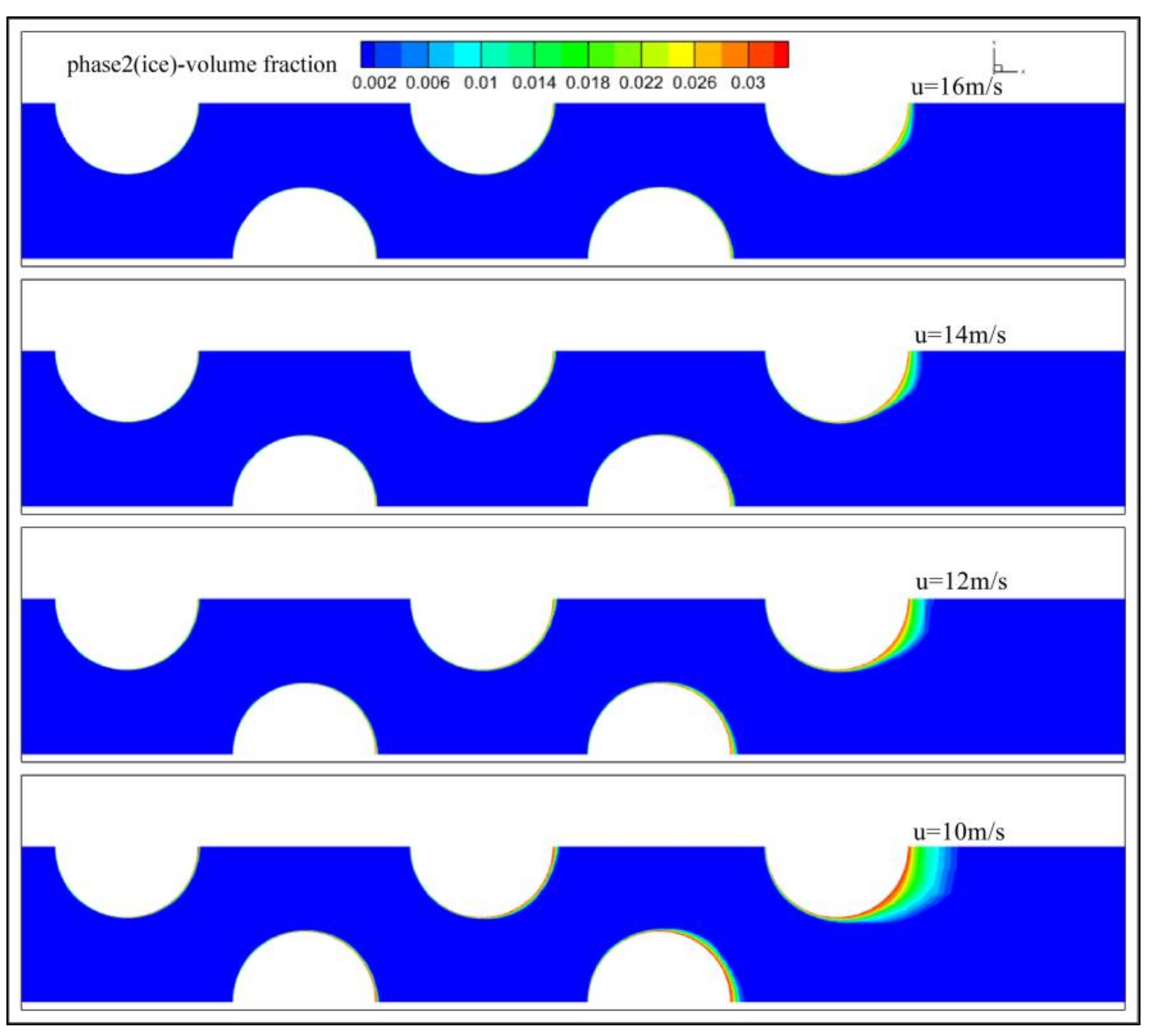
4.2. Frosting at Different Flow Velocity

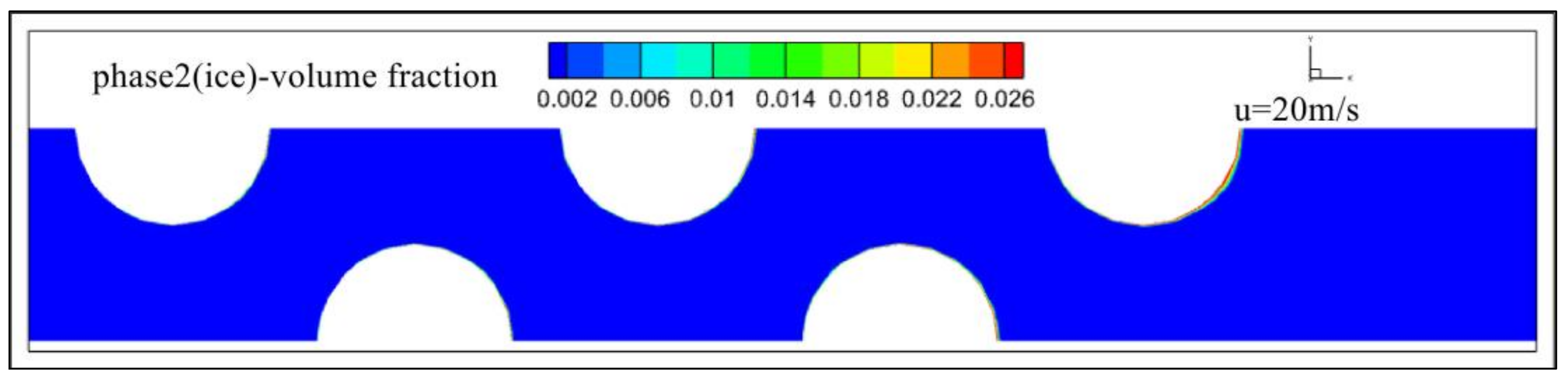
4.2.1. Frost Layer Morphology at Different Flow Velocity

The difference of the frost layer on the tube bundle after 5 min of frosting at different wet airflow velocities was calculated at a wall temperature of 180 K, an inlet wet air temperature of 1473 K, and a moisture content of ${\omega }_{in}=6.4 \mathrm{g}/\mathrm{kg}$. The thickness and density of the frost layer increased with the increase of the calculated time under different flow conditions. The main comparison is the morphology of the frost layer on the 10th row of round tubes. It can be seen that the lower the velocity of the wet air, the greater the thickness of the frost layer formed. As shown in Figure 17: at an inlet velocity of 10 m/s, the thickness of the frost layer formed in the fifth minute was approximately twice as thick as at 12 m/s.

The reasons for the difference in frost morphology were analyzed: firstly, the difference in the inlet flow velocity causes a difference in the velocity distribution during the flow of the wet air between the tube rows. According to the calculation results of single tube frosting, the lower the flow velocity, the larger the low-velocity zone on the backwind side of the circular tube, which is more favorable to the growth of frost layer; secondly, in the process of wet air flowing along the tube bundle, different inlet velocities affect the heat transfer between the tube bundle and the surrounding wet air, which affects the distribution of wet air temperature field, and then affects the morphology of frost layer on each circular tube.

According to the distribution of the frost layer on the tube bundle when the inlet wet air flow rate is 10 m/s frost for 5 min, it can be seen that a certain thickness of the frost layer has been formed on the round tubes of the 8th and 9th rows. If the wet air flow rate is further reduced, a frost layer of significant thickness will also be formed on the round tube near the front row. Additionally, under the condition of a relatively high flow rate (20 m/s), as shown in Figure 18 the increase of frost layer thickness in the whole calculation time is very small, and the effect on the wet air flow rate is also very small.

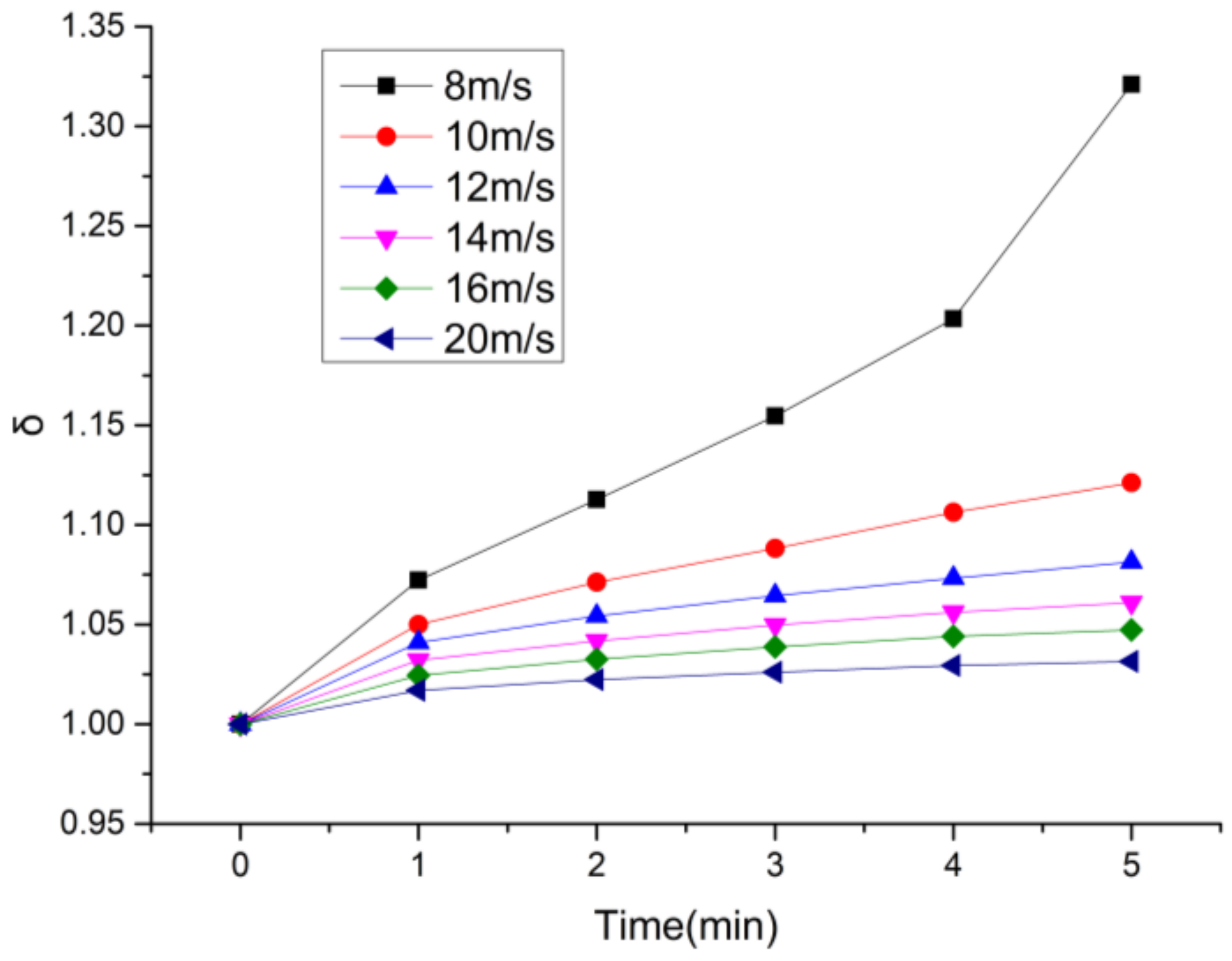
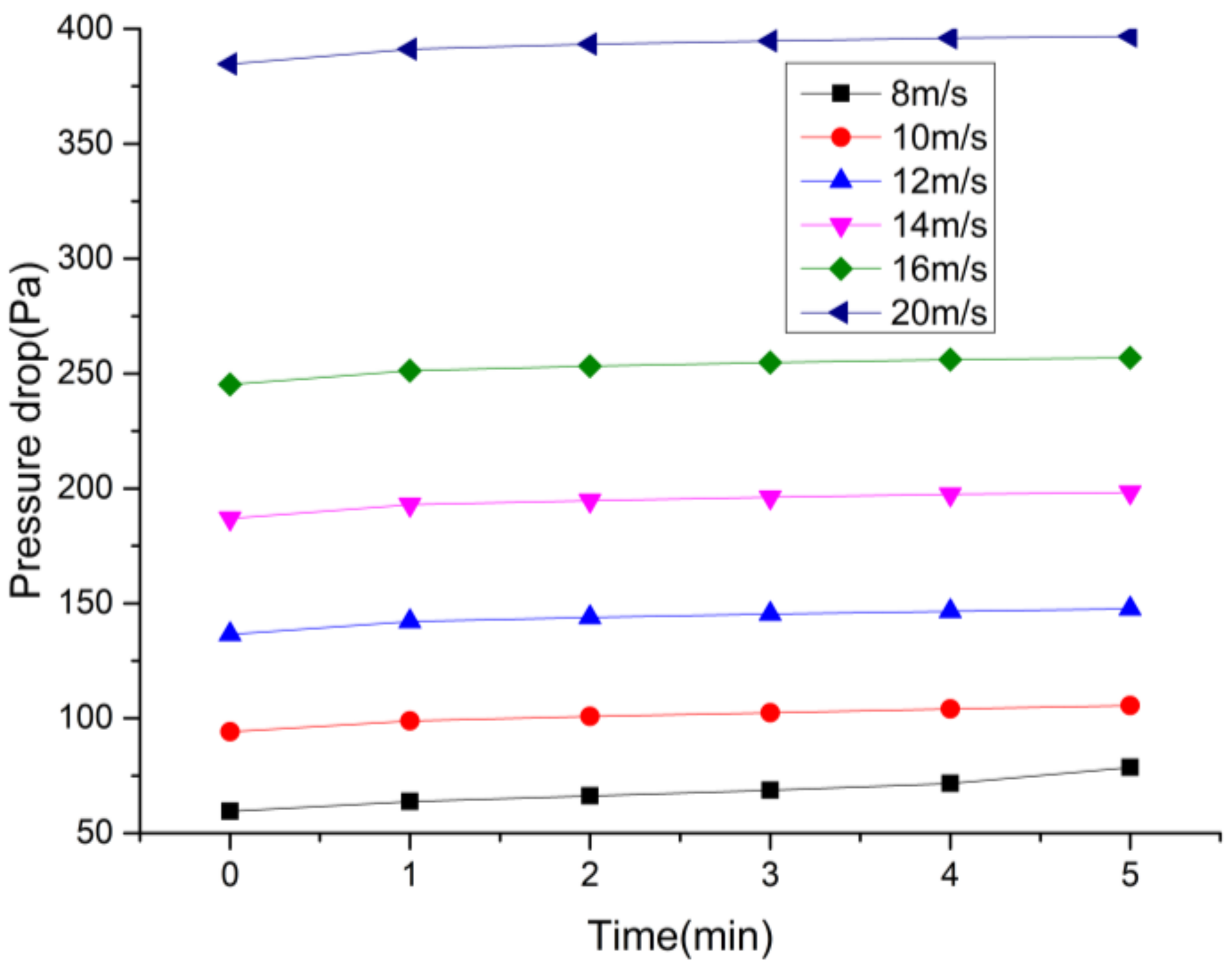
4.2.2. Pressure Drop at Different Flow Velocity

According to the calculation results, the pressure drop caused by frost increases to a certain value under high wet air flow rate conditions and then gradually stabilizes. According to the frost cloud diagram, under the high flow velocity condition, the frost layer grows slowly in the whole calculation time, so the frost layer growth has little effect on the wet air flow field. Under the condition of relatively low flow velocity, the pressure drop of wet air tends to rise throughout the calculation time, and the slope of the curve is larger the lower the flow velocity is. At this time, the thickness of the frost layer formed on the tube bundle is larger and it forms on more round tubes, so the pressure drop continues to increase. The ratio of the pressure drop at each moment of frosting to the pressure drop in the absence of frosting is defined as follows:

$$\mathsf{\delta }=\mathsf{\Delta }\mathrm{P}/\mathsf{\Delta }{P}_0$$

(39)

The pressure drop and the variation of $\delta$ at different flow velocities obtained by numerical calculation are shown in Figure 19 and Figure 20, respectively.

The comparison of $\delta$ with time shows that when the velocity of the wet air is relatively high (e.g., 20 m/s), the value of $\delta$ is about 1 throughout the calculated time. The thickness of the frost layer at each position of the tube bundle is relatively low. Combining the results of numerical calculations of single-tube frosting, it can be seen that under such conditions the mass transfer of water vapor to the ice phase mainly affects the increase in frost density. Additionally, when the flow velocity is relatively low (e.g., 8 m/s), $\delta$ has a value of 1.32 at the 5th min, which is 28.1% higher than at 20 m/s. This indicates that the growth of the frost layer on the tube bundle leads to a significant increase in the pressure drop of the wet air and that the frost layer formed has a gradually increasing effect on the wet air. Additionally, the lower the flow velocity the faster the $\delta$ increases.

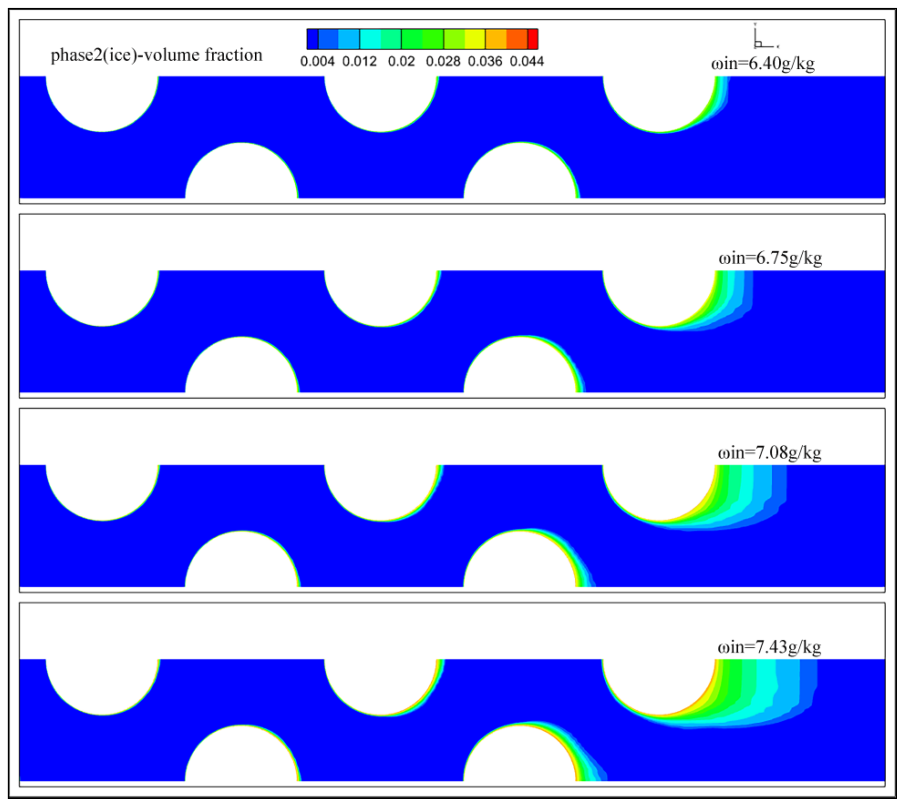
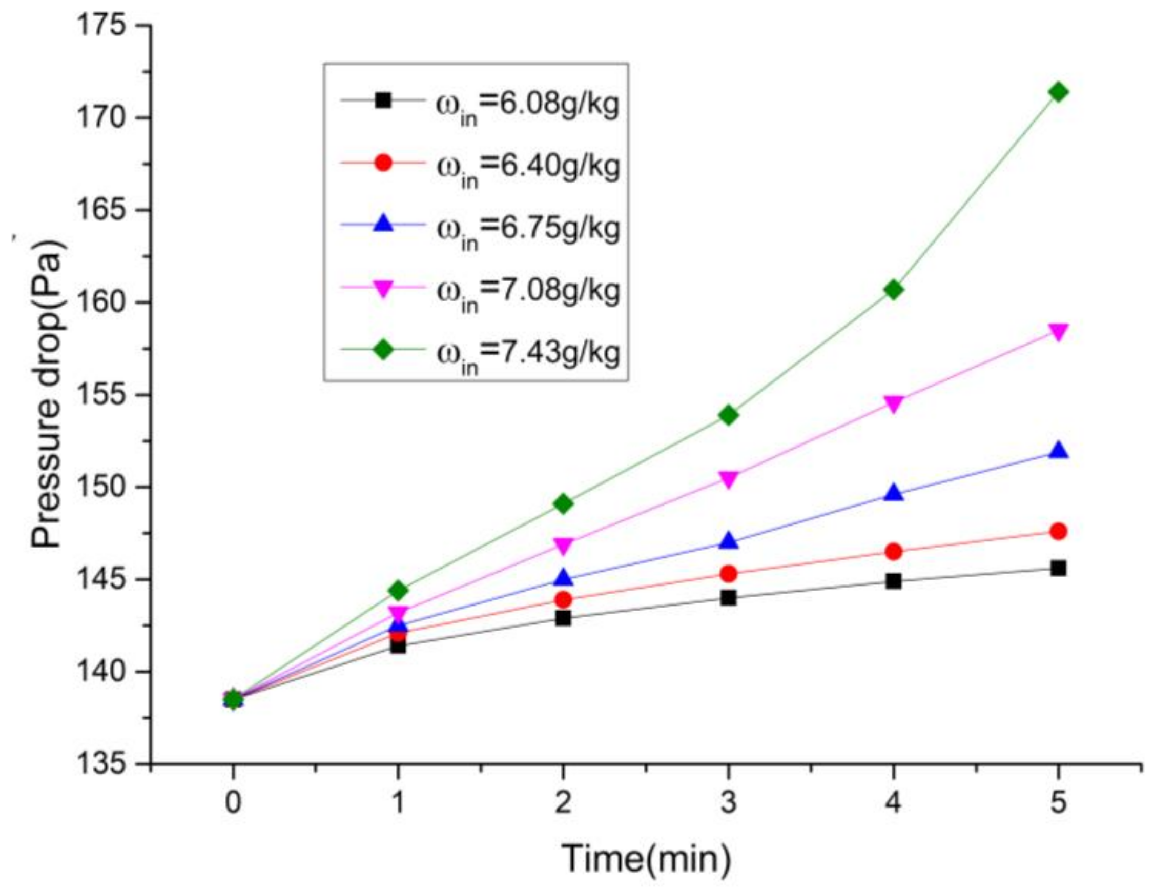
4.3. Frosting under Different Inlet Water Vapor Content

Frost Layer Morphology at Different Water Vapor Content

The difference of frost layer on the tube bundle with different inlet wet air water vapor content (${\omega }_{in}$) was calculated after 5 min at a tube wall temperature of 180 K, an inlet wet air temperature of 1473 K, and a wet airflow velocity of 12 m/s. At the early stage of frosting, there is a significant difference in the thickness of the frost layer formed under different ${\omega }_{in}$(water vapor content of inlet wet air) conditions. As shown in Figure 21, the thickness of the frost layer formed under high ${\omega }_{in}$ conditions are greater than that under low ${\omega }_{in}$ conditions. When ${\omega }_{in}$= 7.08 g/kg, the thickness of the frost layer formed in the 5th minute is about twice as thick as that at ${\omega }_{in}$= 6.75 g/kg. Under the condition of constant wall temperature, the higher the concentration of water vapor at the beginning of frosting, the more the mass transfer of water vapor to the ice phase per unit of time. According to the numerical calculation results of single-tube frosting, it can be seen that the difference in density of the frost layer formed at the beginning of frosting is very small under different ${\omega }_{in}$ inlet conditions, so the increase in mass transfer caused by the difference in water vapor concentration will mainly play a role in increasing the thickness of the frost layer.

Under different ${\omega }_{in}$ conditions, the thickness, and the density of the frost layer formed increased with time as frosting proceeded. When ${\omega }_{in}$ is low, the thickness of the frost layer increases slightly throughout the calculation time, and the frost layer is mainly located on the leeward side of the circular tube and has a thin thickness. The wet air pressure changes slowly throughout the calculation time at low ${\omega }_{in}$. Additionally, when ${\omega }_{in}$ is larger, the frost layer grows significantly at the top and bottom sides of the circular tube, and finally, the thickness of the frost layer approaches the diameter of the circular tube. The wet air pressure drop rate under high ${\omega }_{in}$ condition is higher than when ${\omega }_{in}$ is lower. The results of pressure drop obtained by numerical calculation under different ${\omega }_{in}$ conditions are shown in Figure 22. At lower ${\omega }_{in}$, the pressure drop increases relatively gently, while at higher ${\omega }_{in}$ the pressure drop will increase rapidly. For example, the pressure drop in the 5th minute at ${\omega }_{in}$= 6.085 g/kg increased only 5.1% compared to the unfrosted time. At ${\omega }_{in}$= 7.43 g/kg, this increase is 23.8%.

The effect of different ${\omega }_{in}$ on the frost layer growth is very obvious for two main reasons. First, during the numerical calculation, given a constant wall temperature, the larger ${\omega }_{in}$ is for the same other parameters of the inlet wet air, the greater the driving force of frost formation and the greater the growth rate of the frost layer. Secondly, the density of the frost layer formed at the calculated wall temperature conditions is smaller and the frost layer density is influenced by the ice phase volume number ${\alpha }_i$, ice phase density ${\rho }_i$, wet air volume fraction ${\alpha }_{air}$ and wet air density ${\rho }_{air}$ (${\rho }_i$/${\rho }_{air}$≈ 900). The density of the frost layer mainly depends on ${\rho }_i$, the lower the density the smaller ${\alpha }_i$ can be known, and the variation of ${\omega }_{in}$ mainly affects ${\alpha }_i$.

5. Conclusions

For the frosting problem of combined engine precooler in the working process, a mathematical model of frosting was established to explore the frosting law under different influencing factors. Using the Euler multiphase flow model in Fluent 19 and UDF solution, the variation law of frost on the tube bundle was obtained and summarized as follows.

A CFD-based frost growth and densification model was established. The frost layer and wet air were simulated in the same computational domain, and the frost behavior on the cold wall surface was calculated. By comparing the calculation results and experimental data under different calculation conditions, the thickness of the frost layer and the pressure drop of the wet air are mainly considered, which is in good agreement with the experimental data. The CFD frost layer growth model eliminates the assumption of the initial frost layer thickness and the initial frost layer density, which is more consistent with the actual frost layer formation process.

The shape of the frost layer on the circular tube obtained by numerical calculation is similar to the shape of the frost layer formed under forced convection on the ultra-low temperature surface obtained experimentally in the literature. The effects of wall temperature and inlet wet air parameters on frost formation were obtained by numerical calculations with the fixed-variable method, which are basically consistent with the experimental results obtained in the literature.

Deficiencies and future work: the numerical calculations in this paper have large errors with experimental results at some operating conditions, and no corresponding frosting experiments were performed. The results are compared with the experimental data of forced convection frosting at ultra-low temperature surfaces in the references, and the frosting criterion applies to a limited temperature range. In the future, it is hoped that the frosting criterion can be further improved to obtain a more accurate determination method.

References

1. Mun, H.; Kim, H.; Park, J.; Lee, I. Novel boil-off gas reliquefaction system using liquid air for intercontinental liquefied natural gas transportation. Energy Convers. Manag. 2022, 269, 116078. [Google Scholar] [CrossRef]
2. Brenk, A.; Kielar, J.; Malecha, Z.; Rogala, Z. The Effect of Geometrical Modifications to a Shell and Tube Heat Exchanger on Performance and Freezing Risk During Lng Regasification. Int. J. Heat Mass Transf. 2020, 161, 120247. [Google Scholar] [CrossRef]
3. Liu, S.; Jiao, W.; Ren, L.; Tian, X. Thermal Resistance Analysis of Cryogenic Frosting and Its Effect on Performance of Lng Ambient Air Vaporizer. Renew. Energy 2020, 149, 917–927. [Google Scholar] [CrossRef]
4. Kwon, J.; Yun, S.; Lee, S.; Cho, W.; Kim, Y. Air-Side Heat Transfer Characteristics of Ambient Air Vaporizers with Various Geometric Parameters under Cryogenic Frosting Conditions. Int. J. Heat Mass Transf. 2022, 184, 122245. [Google Scholar] [CrossRef]
5. Liu, S.; Jiao, W.; Wang, H. Three-Dimensional Numerical Analysis of the Coupled Heat Transfer Performance of Lng Ambient Air Vaporizer. Renew. Energy 2016, 87, 1105–1112. [Google Scholar] [CrossRef]
6. Lisowski, F.; Lisowski, E. Finite Element Analysis of Heat Flow through Longitudinal Finned Tubes in the Lng Ambient Air Vaporizer for a Total Frost Case. E3S Web Conf. 2021, 323, 00020. [Google Scholar] [CrossRef]
7. Jadav, C.; Chowdhury, K. Design of Reverse Flow Ambient Air Heated Vaporizer under Different Ambient Temperatures and Optimization of the Fin Arrangement. Therm. Sci. Eng. Prog. 2022, 34, 101426. [Google Scholar] [CrossRef]
8. Kim, K.H.; Ko, H.J.; Kim, K.; Kim, Y.W.; Cho, K.J. Analysis of Heat Transfer and Frost Layer Formation on a Cryogenic Tank Wall Exposed to the Humid Atmospheric Air. Appl. Therm. Eng. 2009, 29, 2072–2079. [Google Scholar] [CrossRef]
9. Li, S.; Ma, T.; Liu, H.; Zhang, Z.; Xiang, Z.; Mo, Z.; Sun, L. Numerical Analysis of Effects of Pre-Cooler Structure Parameter on Its Performance in SABRE. J. Propuls. Technol. 2022, 43, 200818. [Google Scholar]
10. Tanbay, T.; Uca, M.B.; Durmayaz, A. Assessment of Nox Emissions of the Scimitar Engine at Mach 5 Based on a Thermodynamic Cycle analysis. Int. J. Hydrog. Energy 2020, 45, 3632–3640. [Google Scholar] [CrossRef]
11. Tanbay, T.; Durmayaz, A. Exergy and Nox Emission-Based Ecological Performance Analysis of the Scimitar Engine. J. Eng. Gas Turbines Power 2020, 142, 081008. [Google Scholar] [CrossRef]
12. Harada, K.; Tanatsugu, N.; Sato, T. Development Study of a Precooler for the Air-Turboramjet Expander-Cycle Engine. J. Propuls. Power 2001, 17, 1233–1238. [Google Scholar] [CrossRef]
13. Sato, T.; Tanatsugu, N.; Kobayashi, H.; Kimura, T.; Tomike, J.I. Countermeasures against the Icing Problem on the Atrex Precooler. Acta Astronaut. 2004, 54, 671–686. [Google Scholar] [CrossRef]
14. Sato, T.; Tanatsugu, N.; Naruo, Y.; Omi, J.; Tomike, J.I.; Nishino, T. Development Study on Atrex Engine. In Proceedings of the 49th International Astronautical Congress, Melbourne, Australia, 28 September–2 October 1998. [Google Scholar]
15. Hayashi, Y.; Aoki, A.; Adachi, S.; Hori, K. Study of frost properties correlating with frost formation types. J. Heat Transf. 1977, 99, 239. [Google Scholar] [CrossRef]
16. Kim, J.S.; Lee, K.S.; Yook, S.J. Frost Behavior on a Fin Considering the Heat Conduction of Heat Exchanger Fins. Int. J. Heat Mass Transf. 2009, 52, 2581–2588. [Google Scholar] [CrossRef]
17. Choi, S.; Kim, S.J. Effect of Initial Cooling on Heat and Mass Transfer at the Cryogenic Surface under Natural Convective Condition. Int. J. Heat Mass Transf. 2017, 112, 850–861. [Google Scholar] [CrossRef]
18. Yang, D.K.; Lee, K.S. Dimensionless Correlations of Frost Properties on a Cold Plate. Int. J. Refrig. 2004, 27, 89–96. [Google Scholar] [CrossRef]
19. Hermes, C.J. An Analytical Solution to the Problem of Frost Growth and Densification on Flat Surfaces. Int. J. Heat Mass Transf. 2012, 55, 7346–7651. [Google Scholar] [CrossRef]
20. Le Gall, R.; Grillot, J.M.; Jallut, C. Modelling of frost growth and densification. Int. J. Heat Mass Transf. 1997, 40, 3177–3187. [Google Scholar] [CrossRef]
21. Byun, S.; Jeong, H.; Kim, D.R.; Lee, K.S. Frost Modeling under Cryogenic Conditions. Int. J. Heat Mass Transf. 2020, 161, 120250. [Google Scholar] [CrossRef]
22. Cui, J.; Li, W.Z.; Liu, Y.; Zhao, Y.S. A New Model for Predicting Performance of Fin-and-Tube Heat Exchanger under Frost Condition. Int. J. Heat Fluid Flow 2011, 32, 249–260. [Google Scholar] [CrossRef]
23. Cui, J.; Li, W.Z.; Liu, Y.; Jiang, Z.Y. A New Time- and Space-Dependent Model for Predicting Frost Formation. Appl. Therm. Eng. 2011, 31, 447–457. [Google Scholar] [CrossRef]
24. Lee, J.; Kim, J.; Kim, D.R.; Lee, K.S. Modeling of Frost Layer Growth Considering Frost Porosity. Int. J. Heat Mass Transf. 2018, 126, 980–988. [Google Scholar] [CrossRef]
25. Kim, D.; Kim, C.; Lee, K.S. Frosting Model for Predicting Macroscopic and Local Frost Behaviors on a Cold Plate. Int. J. Heat Mass Transf. 2015, 82, 135–142. [Google Scholar] [CrossRef]
26. Wu, X.; Ma, Q.; Chu, F. Numerical Simulation of Frosting on Fin-and-Tube Heat Exchanger Surfaces. J. Therm. Sci. Eng. Appl. 2017, 9, 031007. [Google Scholar] [CrossRef]
27. Afrasiabian, E.; Iliev, O.; Lazzari, S.; Isetti, C. Numerical Simulation of Frost Formation on a Plate-Fin Evaporator. In Proceedings of the 3rd World Congress on Momentum, Heat and Mass Transfer, Budapest, Hungary, 12–14 April 2018. [Google Scholar]
28. Kandula, M. Frost Growth and Densification in Laminar Flow over Flat Surfaces. Int. J. Heat Mass Transf. 2011, 54, 3719–3731. [Google Scholar] [CrossRef]
29. Hermes, C.J.; Piucco, R.O.; Barbosa Jr, J.R.; Melo, C. A Study of Frost Growth and Densification on Flat Surfaces. Exp. Therm. Fluid Sci. 2009, 33, 371–379. [Google Scholar] [CrossRef]
30. Wang, W.; Guo, Q.C.; Lu, W.P.; Feng, Y.C.; Na, W. A Generalized Simple Model for Predicting Frost Growth on Cold Flat Plate. Int. J. Refrig. 2012, 35, 475–486. [Google Scholar] [CrossRef]
31. Jia, Y. Researches on the Flow, Heat Transfer and Frosting for Air Cooling by Mini Tube Bundle at Very Low Temperature. Ph.D. Thesis, Tsinghua University, Beijing, China.
32. Fernandez Villace, V.; Paniagua, G. Simulation of a Variable-Combined-Cycle Engine for Dual Subsonic and Supersonic Cruise. In Proceedings of the 47th AIAA/ASME/SAE/ASEE Joint Propulsion Conference & Exhibit, San Diego, CA, USA, 31 July–3 August 2011. [Google Scholar]
33. Zhukauskas, A. Convective Heat Transfer in Heat Exchangers; Science Publishing House: Beijing, China, 1986. [Google Scholar]
34. Yu, S.; Jones, T.; Ogawa, H.; Karwa, N. Multi-Objective Design Optimization of Precoolers for Hypersonic Airbreathing Propulsion. J. Thermophys. Heat Transf. 2017, 31, 421–433. [Google Scholar] [CrossRef]
Figure 1. Frosting schematic.
Aerospace 09 00630 g001
Figure 2. Variation of saturated water vapor partial pressure with temperature.
Aerospace 09 00630 g002
Figure 3. Simulation flow chart.
Aerospace 09 00630 g003
Figure 4. Frost density validation results.
Aerospace 09 00630 g004
Figure 5. Frost layer thickness verification results.
Aerospace 09 00630 g005
Figure 6. Tube frosting verification.
Aerospace 09 00630 g006
Figure 7. Comparison of frost morphology((a):Present model,(b):Experimental results).
Aerospace 09 00630 g007
Figure 8. Tube bundle structure and tube spacing.
Aerospace 09 00630 g008
Figure 9. Schematic diagram of the computational domain.
Aerospace 09 00630 g009
Figure 10. Grid division and local encryption.
Aerospace 09 00630 g010
Figure 11. Variation of the maximum ice phase volume fraction at 5 min for different grid numbers.
Aerospace 09 00630 g011
Figure 12. Variation of frost morphology on the tube bundle.
Aerospace 09 00630 g012
Figure 13. Variation of wet air flow rate after frosting.
Aerospace 09 00630 g013
Figure 14. Pressure drop after frosting.
Aerospace 09 00630 g014
Figure 15. Frost morphology at different wall temperatures (5th min).
Aerospace 09 00630 g015
Figure 16. Pressure drop at different wall temperatures.
Aerospace 09 00630 g016
Figure 17. Frost morphology at different flow velocity (5th min).
Aerospace 09 00630 g017
Figure 18. Frost morphology at flow velocity 20 m/s (5th min).
Aerospace 09 00630 g018
Figure 19. Pressure drop at different flow rates.
Aerospace 09 00630 g019
Figure 20. At different flow rates.
Aerospace 09 00630 g020
Figure 21. Frost morphology at different moisture contents (5th min).
Aerospace 09 00630 g021
Figure 22. Variation of pressure drop with different ω i n .
Aerospace 09 00630 g022