Learning-Based Pose Estimation of Non-Cooperative Spacecrafts with Uncertainty Prediction

Abstract

Estimation of spacecraft pose is essential for many space missions, such as formation flying, rendezvous, docking, repair, and space debris removal. We propose a learning-based method with uncertainty prediction to estimate the pose of a spacecraft from a monocular image. We first used a spacecraft detection network (SDN) to crop out the rectangular area in the original image where only spacecraft exist. A keypoint detection network (KDN) was then used to detect 11 pre-selected keypoints with obvious features from the cropped image and predict uncertainty. We propose a keypoints selection strategy to automatically select keypoints with higher detection accuracy from all detected keypoints. These selective keypoints were used to estimate the 6D pose of the spacecraft with the EPnP algorithm. We evaluated our method on the SPEED dataset. The experiments showed that our method outperforms heatmap-based and regression-based methods, and our effective uncertainty prediction can increase the final precision of the pose estimation.

1. Introduction

For the demands of some space missions, such as maintenance for spacecrafts [1], on-orbit docking [2] and removing space debris [3], the pose estimation for non-cooperative spacecrafts has been a hot topic. Non-cooperative spacecrafts generally refer to spacecrafts that do not provide effective cooperative information, including malfunctioning or failed satellites, space debris, and opposing spacecrafts. In the past, the pose of spacecrafts was usually estimated by high-precision sensors [4,5,6]. However, due to the high costs and power consumption of these sensors, this solution of pose estimation is not applicable to many low-cost spacecrafts [7]. Monocular images can provide the key position and orientation information required by the navigation system for spacecraft under low power [8].

In this paper, we mainly focus on how to estimate the 6D pose of a spacecraft from a monocular image. The main difficulty of this task is the limited amount of available pose information. Moreover, the complex shooting environment in space, such as illumination and backgrounds, also brings more challenges. Dhome proposed a closed model-based 6D pose image recognition method [9]. This method corresponds all possible 3D model edges to the captured 2D image edges one by one and uses soft assign to avoid the computational overload caused by exhaustive enumeration. Following Dhome, Kanani and Petit made partial improvements to improve its computational speed and reduce data dependence [10,11]. These methods were initially applied to ground-based robotic navigation algorithms and later to satellite-based monocular navigation. However, model-based methods require a large amount of feature matching before solving the positional pose, which is difficult to apply in real time [12]. Therefore, some people proposed a non-model-based method to estimate the 6D pose. Augenstein and Rock proposed to use SIFT-based SLAM for pose solution of spacecrafts [13]. Nevertheless, non-model-based approaches have the possibility of losing target features due to large changes in image conditions or perspective relationships [14]. The pose estimation methods have been further developed with the further development of image recognition algorithms. D’Amico proposed a perceptual organization of detected edges in images using the Sobel algorithm and the Hough algorithm to solve the pose-initialization problem [15]. For the first time, pose estimation of a fully non-cooperative spacecraft has been achieved. However, this method is computationally expensive, difficult to use in real-time on onboard hardware, and lacks robustness to illumination conditions [15]. Sharma improved D’Amico’s research by proposing Sharma-Ventura-D’Amico (SVD) architecture and introducing the weak gradient elimination (WEG) to reduce the search space [12]. Sharma’s method reduces the computation time and improves the detection accuracy, but has the drawback of generating spurious edges when the image condition is bad.

In recent years, due to the development of deep learning algorithms, especially the neural networks, there have been new advances in pose estimation for spacecrafts from monocular images. It has been shown that feature detected by CNNs has more accuracy and stability than traditional methods for computer vision domain tasks [16]. Therefore, many learning-based methods have been proposed to solve the pose estimation problem [17,18,19,20,21,22,23]. Recently, Chen and Park proposed a similar pipeline to estimate the 6D pose of spacecrafts from a monocular image [18,19]. They used CNNs to automatically crop out the part of image where the spacecraft exists and predicted the 2D pixel coordinates of keypoints from the cropped image. They used the 2D pixel coordinates of keypoints and a wireframe model of the spacecraft obtained in advance to estimate the 6D pose. Following their work, we propose a learning-based 6D pose estimation method for spacecrafts, with effective uncertainty prediction enabling automatic selection of keypoints for pose estimation. Our main contribution can be concluded as follows:

•

We introduce the idea of region detection into the keypoint detection of spacecrafts, which can capture the feature of keypoints better;

•

We achieve effective uncertainty prediction for the detected keypoints, which can be used to automatically eliminate keypoints with low detection accuracy;

•

We conduct sufficient experiments on SPEED dataset [17]. Compared with previous methods, our method can reduce the average error of pose estimation by 53.3% while reducing the number of model parameters.

The rest of this paper is organized as follows. First, in Section 2 we briefly introduce previous works on learning-based 6D pose estimation of spacecraft and the keypoints detection. Second, the proposed methods are detailed in Section 3. Third, the experimental results will be benchmarked in Section 4. Finally, Section 5 will conclude this work.

2. Related Work

2.1. Learning-Based Methods

Instead of handcrafting the image features to estimate the pose of spacecraft, learning-based methods use deep learning to automatically extract the features to estimate the 6D pose of the spacecraft. These methods can be divided into two categories, direct estimation and indirect estimation. Sharma [22] used a CNN to extract the features in images and a fully connected layer to output a 6-dimensional vector as the predicted 6D pose. In Gao’s work [21], the prediction of the orientation vector was converted into the regression of a heatmap. Sharma adopted multi-task learning [20,23] to estimate 6D pose. While predicting the 6D pose, he completed the task of keypoints prediction, spacecraft detection and image segmentation simultaneously. For the indirect estimation methods, Park [18] and Chen [19] first used CNN to predict the position of keypoints and then took these keypoints to estimate pose with the EPnP algorithm [24]. They mainly differ in how to detect the keypoints. Park [18] used light MobileNetv2 [25] as a backbone to extract features and used a fully convolutional network (FCN) [26] to regress the pixel coordinates of keypoints. Chen [19] predicted a heatmap for each keypoint, meaning the probability of keypoints appearing at each pixel coordinate.

Our method also belongs to the method of indirect prediction. Different from [18,19], we treat each keypoint as a square region to detect. Although Chen also treated each keypoint as a square region, the size of the area he set is fixed. We replace three square anchors of different sizes for each pixel on the feature map for the situation of different relative distance to the spacecraft (Figure 1).

2.2. Keypoint Detection

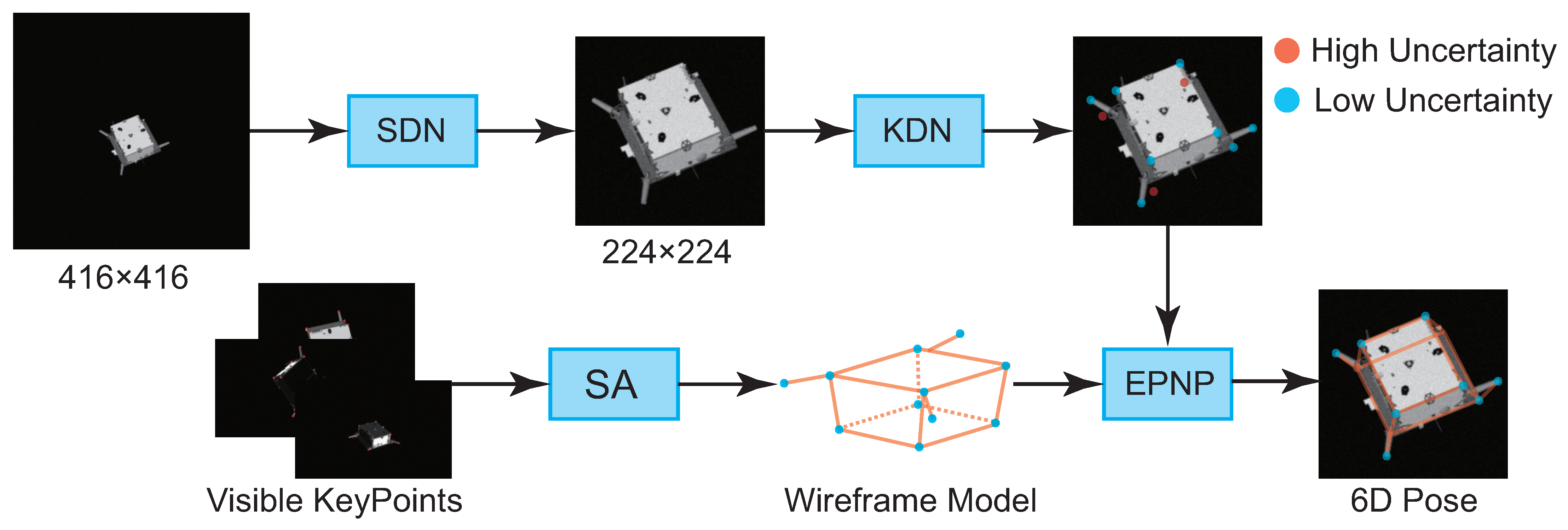
Keypoint detection is a traditional task in computer vision, and there have been many surveys that extensively discuss related methods [27]. We present related works in two main categories: handcrafted and learned detector.

For handcrafted detectors, Harris [28] and Hessian [29] detectors used first and second order image derivatives to find corners or blobs in images. The more refined keypoint feature can be calculated through some engineered algorithms [30,31,32,33], which seek alternative structures within images to represent the keypoint. MSER [32] segmented and selected stable regions as keypoints, and SIFT [30] looked for blobs over multiple scale levels.

For learned detectors, the improvement of learned methods in object detection help to explore similar techniques for keypoint detectors. FAST [34] was one of the first attempts to use machine learning to design a keypoint feature descriptor, and then some people made improvements on this method [31,35,36]. Recently, many methods have been proposed to utilize CNNs to detect keypoints. TILDE [37] trained multiple patch-wise linear regression models to detect keypoints that are robust under severe weather and illumination changes. Georgakis [38] proposed a pipeline to automatically sample positive and negative pairs of patches from a region proposal network to optimize jointly point detections and their representations. LF-Net [39] estimated the position, scale and orientation of features by jointly optimizing the detector and descriptor.

For the keypoint detection of spacecrafts, Park [19] directly used CNN to regress the 2D coordination of keypoints. Sharma [23] and Park [23] improved it by introducing multitask learning. Chen used HRNet [40], a CNN proposed to predict the pose of the human body, to predict the heatmap of the monocular image. However, he assigned the same region for all the keypoints, which is not rational for different relative distances. We introduce the idea of region detection into the keypoint detection task of spacecraft, where anchors of different sizes can fit different relative distances (Figure 1). At the same time, an effective uncertainty prediction is introduced for detected keypoints, enabling end-to-end accurate keypoint selection.

3. Method

The overall pipeline of our method is shown in Figure 2. We first selected 22 images from multiple views to manually obtain the 2D coordinates of each keypoint, and used the simulated annealing (SA) algorithm [41] to obtain the spacecraft’s 3D wireframe model. For each input image, we first used a spacecraft detection network (SDN) to find the location and the area where the spacecraft exists. Then, the cropped image of the spacecraft was put into a keypoint detection network (KDN) to detect the position of keypoints. KDN simultaneously estimates the uncertainty of detection for each keypoint. We developed a strategy to select more accurate keypoints as candidate keypoints. The reconstructed 3D coordinate and predicted 2D coordinates of all the candidate keypoints were used to solve the 6D pose of spacecrafts through EPnP [24].

3.1. 3D Wireframe Model Recovery

Given the internal parameter matrix $K_c$ and the external parameter matrix R and T of the monocular camera, if the 3D coordinate $p_{3D,k}$ of the k-th keypoint in the world coordinate system is known, we can obtain its 2D coordinate in the image. We selected 11 keypoints with great visibility. For each keypoint, we obtained its 2D coordinate manually from 22 images. For each k-th keypoint, the sum of the reprojection error was minimized over a set of images in which the k-th keypoint was visible. The optimal 3D coordinate of each keypoint can be obtained by minimizing the following objective function,

$$\underset{p_{3D,k},{\left\{{\lambda }_{i,k}\right\}}_{i=1}^N}{min}\sum _i{∥{\lambda }_{i,k}{p}_{2D,i,k}^h-K_c\left[R_i\left|T_i\right.\right]p_{3D,k}^h∥}_2,$$

(1)

where $R_i$ and $T_i$ represent the known camera extrinsic parameters. $p_{2D,i,k}^h$ represents the 2D coordinate of the k-th keypoint in the i-th image and $p_{3D,k}^h$ represents the according 3D coordinate. The superscript h indicates that the point is expressed in homogenous coordinates. ${\lambda }_{i,k}$ represents the scaling factor, which is also needed to solve. N is the number of selected images for k-th keypoint. We define the symbols in Equation (1) in more detail as:

$$K_c\left[R_i\left|T_i\right.\right]=P_i=\left[\begin{array}{cccc}{p}_i^{11}& p_i^{12}& p_i^{13}& p_i^{14}\\ p_i^{21}& p_i^{22}& p_i^{23}& p_i^{24}\\ p_i^{31}& p_i^{32}& p_i^{33}& p_i^{34}\end{array}\right],p_{2D,i,k}^h=\left[\begin{array}{c}{u}_{i,k}\\ v_{i,k}\\ 1\end{array}\right],p_{3D,k}^h=\left[\begin{array}{c}{X}_k\\ Y_k\\ Z_k\\ 1\end{array}\right].$$

(2)

where $p_i^{**}$ represents the element in matrix $P_i$. The $(u_{i,k},v_{i,k})$ represents the pixel coordinate of the k-th keypoint in the i-th image. The $(X_k,Y_k,Y_k)$ represents the 3D coordinate of the k-th keypoint in the world coordinate system.

Due to the presence of noise, the optimal solution cannot make the Equation (1) zero. The most general way is to use the least square (LS) method to obtain the optimal solution. According to Equation (1), we can construct N linear equations with N images as:

$$\left\{\begin{array}{c}(u_{i,k}{p}_i^{31}-p_i^{11})X_k+(u_{i,k}{p}_i^{32}-p_i^{12})Y_k+(u_{i,k}{p}_i^{33}-p_i^{13})Z_k=p_i^{14}-u_{i,k}{p}_i^{34}\\ (v_{i,k}{p}_i^{31}-p_i^{21})X_k+(v_{i,k}{p}_i^{32}-p_i^{22})Y_k+(v_{i,k}{p}_i^{33}-p_i^{23})Z_k=p_i^{24}-v_{i,k}{p}_i^{34}\end{array}.\right.$$

(3)

Thus, we can construct over-determined linear equations for $s={\left(X_k,Y_k,Z_k\right)}^T$ as:

$$As=b,$$

(4)

where A is a $2N\times 3$ matrix and b is a $2N\times 1$ matrix, i.e.,

$$A=\left[\begin{array}{c}\begin{array}{ccc}{u}_{1,k}{p}_1^{31}-p_1^{11}& u_{1,k}{p}_1^{32}-p_1^{12}& u_{1,k}{p}_1^{33}-p_1^{13}\end{array}\\ \begin{array}{ccc}{v}_{1,k}{p}_1^{31}-p_1^{21}& v_{1,k}{p}_1^{32}-p_1^{22}& v_{1,k}{p}_1^{33}-p_1^{23}\end{array}\\ ⋮\\ \begin{array}{ccc}{u}_{N,k}{p}_N^{31}-p_N^{11}& u_{N,k}{p}_N^{32}-p_N^{12}& v_{N,k}{p}_N^{33}-p_N^{23}\end{array}\\ \begin{array}{ccc}{v}_{N,k}{p}_N^{31}-p_N^{21}& v_{N,k}{p}_N^{32}-p_N^{22}& v_{N,k}{p}_N^{33}-p_N^{23}\end{array}\end{array}\right],b=\left[\begin{array}{c}{p}_1^{14}-u_{1,k}{p}_1^{34}\\ p_1^{24}-v_{1,k}{p}_1^{34}\\ ⋮\\ p_N^{14}-u_{N,k}{p}_N^{34}\\ p_N^{24}-v_{N,k}{p}_N^{34}\end{array}\right]$$

(5)

.

The optimal solution can be obtained by the LS as:

$$s={\left(A^{T}A\right)}^{-1}{A}^{T}b.$$

(6)

In this paper, we mainly consider that the manually chosen 2D coordinates of the keypoints may have different degrees of error in different images. We selected only 12 out of 22 images for each keypoint to obtain its 3D coordinates, which makes Equation (1) reach the least value. We used SA [41] to obtain the 3D ordinates $p_{3D,k}^h$ and the scaling factors ${\lambda }_{i,k}$, and calculated the value of Equation (1) to select the best 12 images for each keypoint. In Section 4.6, we show that compared to obtaining the optimal solution directly through LS, the SA method can achieve a better solution.

After obtaining the wireframe model of spacecraft, we can obtain the 2D coordinates of keypoints in each image without manually labeling a large number of images for subsequent tasks.

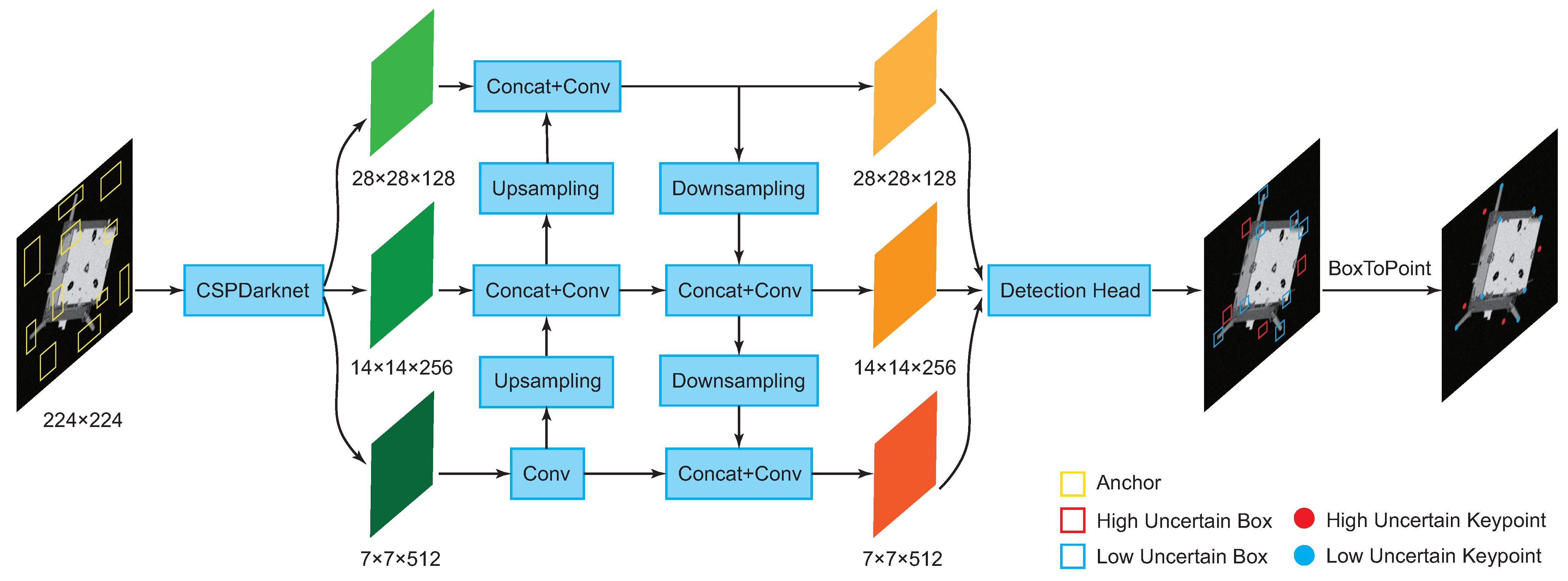
3.2. Spacecraft Detection Network (SDN)

We used a Spacecraft Detection Network (SDN) to automatically find the location of the spacecraft. Considering the smaller model consumes less, we took the tiny version of YOLOX [42] as our SDN. The 2D bounding boxes were obtained by projecting the 3D keypoints onto the image using the ground-truth poses. In order to ensure that the bounding boxes could contain the whole spacecraft, we enlarged the boxes by 10% in the center as our final labels.

3.3. Keypoints Detection Network (KDN)

We treated each keypoint as a square region and used anchor-based methods to detect them. Different from the general object detection method, where we needed to replace rectangular boxes of different sizes for each pixel, since our detection area was square, we only replaced three square boxes with different sizes for each pixel to adapt to the different relative distances of the spacecraft from the camera. The framework of the KDN is shown in Figure 3. We used CSPDarknet [43] as the backbone to extract features of three scales from the input image. We used the feature pyramid network (FPN) [44] to complement the features between different scales to obtain refined features. Finally, all features were input to the detection head for keypoint detection.

For the detection and classification, we minimized the following loss function, commonly used in object detection [43], i.e.,

$$L_{det}=\frac{1}{N}\sum _{i=1}^N\left(L_{reg}(b_i,{\tilde{b}}_i)+L_{cls}(c_i,{\tilde{c}}_i)+L_{conf}(C_i,{\tilde{C}}_i)\right),$$

(7)

where $b_i$, $c_i$ and $C_i$ represent the box, keypoint class and confidence predicted by the KDN for the i-th image, respectively. ${\tilde{b}}_i$, ${\tilde{c}}_i$ and ${\tilde{C}}_i$ represent the corresponding labels. $L_{reg}(•)$ represents the MSE loss function, $L_{cls}(•)$ and $L_{conf}(•)$ represent the cross entropy loss function, and N represents the number of images in each batch.

We define the predicted box $b_i$ and label ${\tilde{b}}_i$ as:

$$\left\{\begin{array}{c}{b}_i=\left[\begin{array}{cccc}{x}_i& y_i& w_i& h_i\end{array}\right]\\ {\tilde{b}}_i=\left[\begin{array}{cccc}{\tilde{x}}_i& {\tilde{y}}_i& {\tilde{w}}_i& {\tilde{h}}_i,\end{array}\right]\end{array}\right.$$

(8)

where $(x_i,y_i)$ represent the pixel coordinates of the center point of the predicted box on the image, and $w_i$ and $h_i$ represent the width and height of the predicted box, respectively. The symbols with superscript ${}^{\sim }$ represents the corresponding label. The $L_{reg}(b_i,{\tilde{b}}_i)$ can be written as:

$$L_{reg}(b_i,{\tilde{b}}_i)={(x_i-{\tilde{x}}_i)}^2+{(y_i-{\tilde{y}}_i)}^2+{(\sqrt{w_i}-\sqrt{{\tilde{w}}_i})}^2+{(\sqrt{h_i}-\sqrt{{\tilde{h}}_i})}^2.$$

(9)

For $L_{cls}(c_i,{\tilde{c}}_i)$, both the predicted keypoint class $c_i$ and label ${\tilde{c}}_i$ are 11-dimensional column vectors. For $c_i$, each element $c_{i,k}$ represents the probability that the k-th keypoint exists in the box. Each element ${\tilde{c}}_{i,k}$ in ${\tilde{c}}_i$ represents the corresponding label. The $L_{cls}(c_i,{\tilde{c}}_i)$ can be written like cross entropy loss function as:

$$L_{cls}(c_i,{\tilde{c}}_i)=-\sum _{k=1}^K[{\tilde{c}}_{i,k}{log}_2\left(c_{i,k}\right)+(1-{\tilde{c}}_{i,k}){log}_2(1-c_{i,k})].$$

(10)

For the uncertainty prediction, we minimized the following loss function,

$$L_{uncertain}=\frac{1}{N}\sum _{i=1}^N{L}_{uncertain}(U_i,{\tilde{U}}_i),$$

(11)

where $U_i$ represents predicted uncertainty, i.e., the probability of whether there is a target for each keypoint, and ${\tilde{U}}_i$ represents the corresponding label. $L_{uncertain}(U_i,{\tilde{U}}_i)$ can be written as:

$$L_{uncertain}(U_i,{\tilde{U}}_i)=\frac{1}{K}\sum _{k=1}^K[-{\tilde{U}}_{i,k}{log}_2{U}_{i,k}-(1-{\tilde{U}}_{i,k}){log}_2(1-U_{i,k})],$$

(12)

where $U_{i,k}$ represents predicted uncertainty for the k-th keypoint, and ${\tilde{U}}_{i,k}$ represents the corresponding label. The uncertainty label for the k-th keypoint can be calculated as:

$${\tilde{U}}_{i,k}=\left\{\begin{array}{cc}1& \frac{L_{cls}(c_{i,k},{\tilde{c}}_{i,k})}{logK}>1\\ \frac{1-IOU(b_{i,k},{\tilde{b}}_{i,k})+\frac{L_{cls}(c_{i,k},{\tilde{c}}_{i,k})}{logK}}{2}& else,\end{array}\right.$$

(13)

where $IOU(•)$ is the intersection ratio of the predicted box $b_i$ and the ground truth box ${\tilde{b}}_i$. K is the number of keypoint classes. The subscript k indicates that the variable is related to the k-th keypoint.

In order to guide KDN to achieve the joint prediction of classification uncertainty and regression uncertainty, the loss function of our KDN is defined as:

$$L=L_{det}+L_{uncertain}.$$

(14)

3.4. Pose Estimation

After obtaining the 3D coordinates and 2D coordinates of the keypoints, we used the EPnP [24] to solve the 6D pose of the spacecraft. To increase the accuracy of pose estimation, we developed a strategy to select more accurate keypoints by the predicted uncertainty. We divided the selection strategy into two separate sub-strategies, Top K and uncertainty threshold selection (UTS).

For each category of keypoints, the keypoint with the lowest uncertainty was used as the final detected keypoint of this category. In UTS strategy, for these eleven detected keypoints, we selected the keypoints whose uncertainty was less than a given threshold $\mu$ as candidate keypoints. In Top K strategy, if the number of candidate keypoints was less than five, we directly used the five keypoints with the lowest uncertainty among the eleven detected keypoints as candidate keypoints, since four keypoints may be coplanar, which is detrimental to the pose estimation. If the number of candidate keypoints was more than $K_n$, we took the $K_n$ keypoints with the lowest uncertainty as candidate keypoints. All the candidate keypoints were used to solve the 6D pose with EPnP [24]. The above architecture is described in Algorithm 1.

Algorithm 1 Keypoints selection strategy

Require: Keypoints with predicted uncertainty $\left\{p_{2D,i,k},U_{i,k}\right\}$, uncertainty threshold $\mu$, candidate keypoints set C, detected keypoints set D and $K_n$. $C\leftarrow ⌀$. $D\leftarrow ⌀$. for$m=1$ to 11 do    $\left\{p_{2D,m},U_m\right\}\leftarrow \left\{p_{2D,i,m},U_{i,m}\right\}$ with the smallest $U_{i,m}$.    Add $\left\{p_{2D,m},U_m\right\}$ into D. end for $N\leftarrow 0$. # Conduct UTS strategy. for$m=1$ to 11 do    if $U_m<\mu$ then      Add $\left\{p_{2D,m},U_m\right\}$ into C from D.      $N\leftarrow N+1$.    end if end for # Conduct Top K strategy. while$N>K_n$do    Remove $\left\{p_{2D,m},U_m\right\}$ with the biggest $U_m$ from C.    $N\leftarrow N-1$. end while while$N<5$do    Add $\left\{p_{2D,m},U_m\right\}$ with the smallest $U_m$ from D into C.    $N\leftarrow N+1$. end while returnC.

4. Experiments

4.1. Datasets and Implementation Details

We evaluated our method using the SPEED dataset [17] with 12,000 synthetic satellite images and five real satellite images provided by the Advanced Concepts Team (ACT) at European Space Agency (ESA) in the pose estimation challenge 2019 [45,46]. Each image was annotated with the extrinsic parameter matrices R and T corresponding to the camera. The difficulty of pose estimation varied from image to image. They had varying degrees of light intensity, relative distance to spacecraft, perspective occlusion, and background complexity (Figure 4). From the synthetic images of SPEED dataset, we randomly selected 10,000 images as the training set and 1000 images as the validation set. The rest 1000 synthetic images were used as the test set, as well as five real images.

We took the methods of Park [18] and Chen [19] as our baselines. Their methods share a similar pipeline with ours, and the main difference is how to predict the 2D coordinates of keypoints. Park [18] used CNNs to directly regress the 2D coordinates of keypoints, which belong to the regression-based method. Chen [19], however, predicted a heatmap for each keypoint, indicating the probability of each keypoint appearing at different positions, which is a heatmap-based method. We introduce the idea of region detection for the prediction of keypoint positions. We hope to prove the superiority of our method for improving the accuracy of 6D pose estimation by comparing it with the above methods. In order to ensure the fairness of the comparison, all three methods used the data augmentation method used by Park and were trained with the Adaptive Momentum Estimation (Adam) optimizer for 300 epochs with a 0.001 learning rate, 48 batch-size, momentum of 0.9, and weight decay of $5\times {10}^{-4}$.

In Section 4.3, we set $K_n$ and $\mu$ as 7 and 0.5, following Algorithm 1.

4.2. Evaluation Metrics

In order to quantitatively evaluate our final pose estimation results, we adopt the evaluation metrics provided by ESA to define the errors of estimation of translation, orientation and 6D pose.

For the i-th image, the error of the pose estimation is calculated as the sum of the orientation error $E_{R,i}$ and the translation error $E_{T,i}$, i.e.,

$$E_i=E_{R,i}+E_{T,i}.$$

(15)

The translation error and orientation error can be calculated as:

$$E_{T,i}=\frac{{∥t_i-{\tilde{t}}_i∥}_2}{{∥t_i∥}_2},E_{R,i}=2arccos(<{\tilde{q}}_i,q_i>),$$

(16)

where $t_i$ and ${\tilde{t}}_i$ represent the predicted and real translation vectors, and $q_i$ and ${\tilde{q}}_i$ represent the predicted and real orientation vectors, respectively. ${∥•∥}_2$ is to calculate the two-norm of a vector and $〈•,•〉$ is to calculate the angle between two vectors. The mean error of the pose estimation for the test set is calculated as:

$$meanE=\frac{1}{N}\sum _{i=1}^N{E}_i,$$

(17)

where N is the number of images in the test set. Similarly, we can calculate the mean and median of other errors on the test set. We take the above six metrics, $median{E}_T$, $median{E}_R$, $medianE$, $mean{E}_T$, $mean{E}_R$ and $meanE$, to evaluate the pose estimation results.

4.3. Comparison

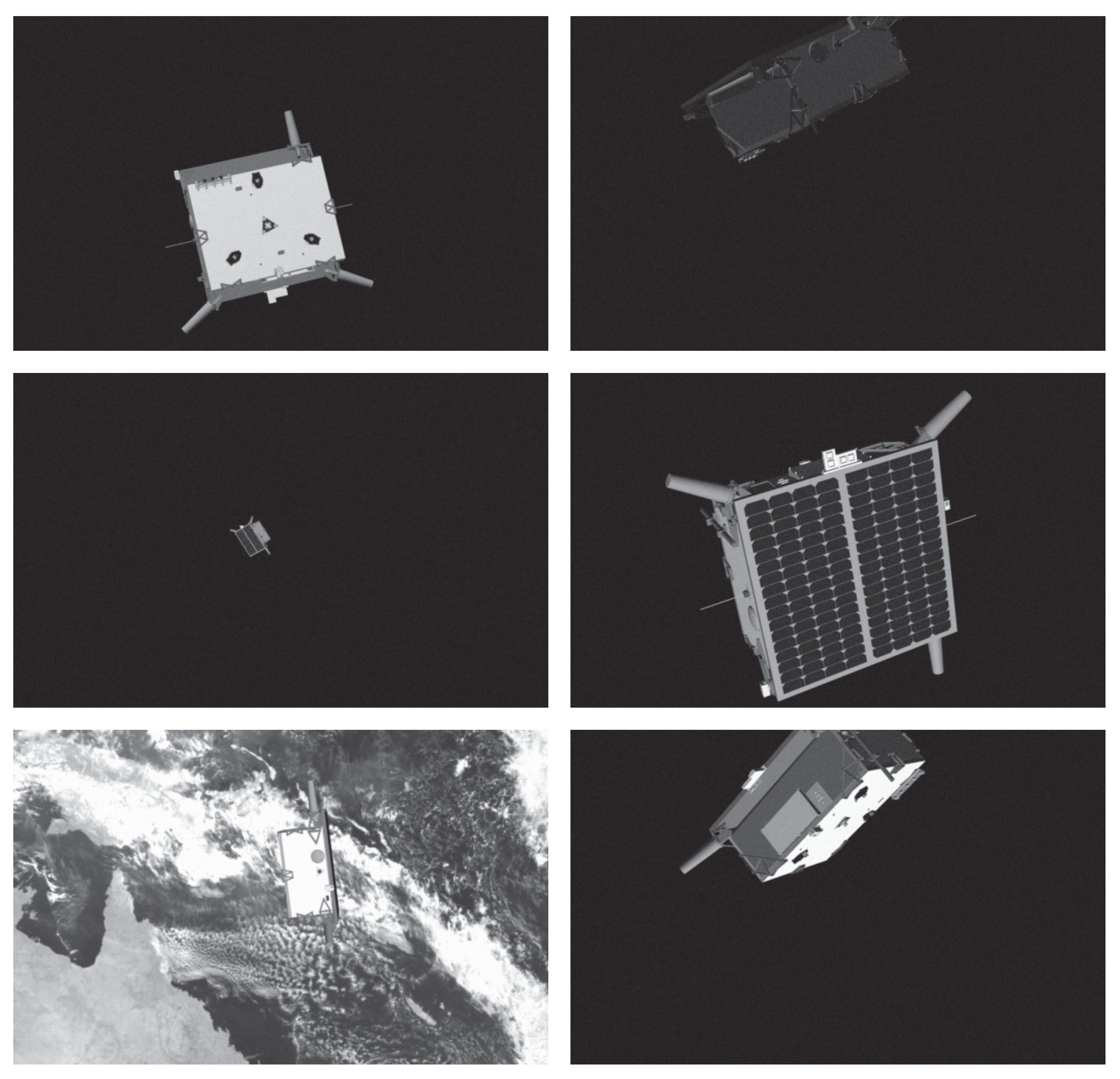
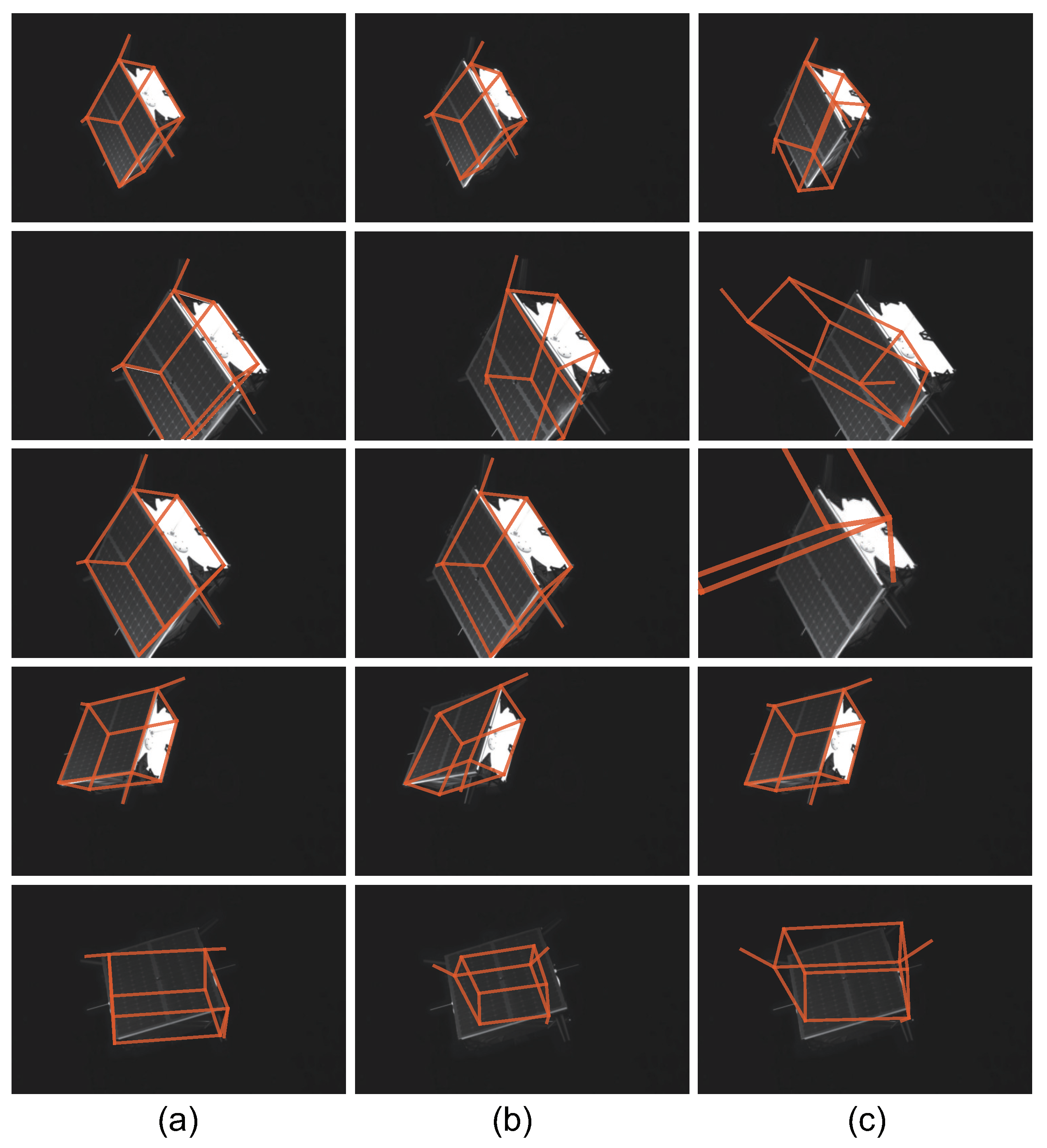
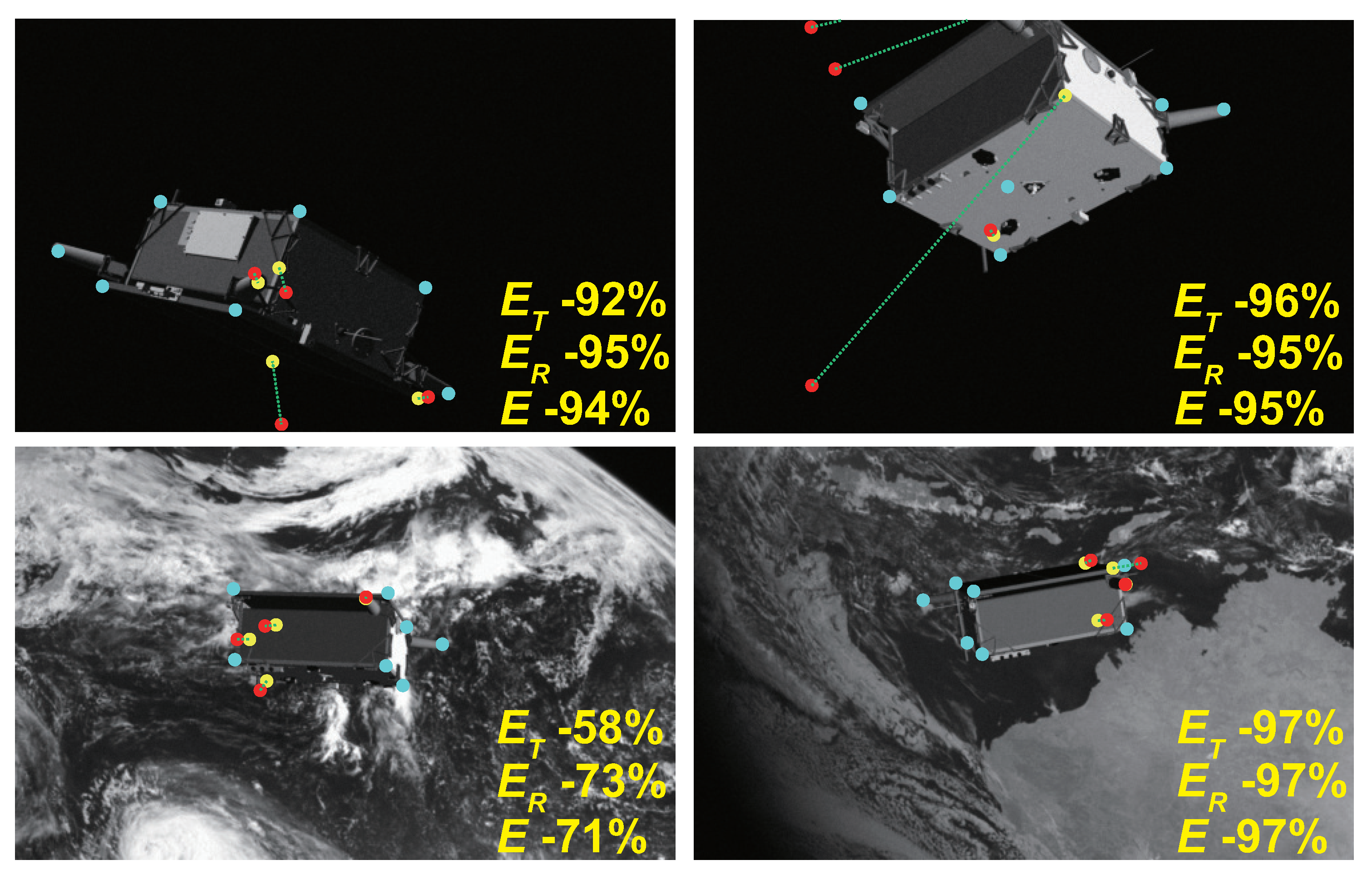
4.3.1. Comparison in Synthetic Images

In this section, we compare three methods in 1000 synthetic images (

Table 1. The performance of three methods on 1000 synthetic images. Ours-small means that we reduce the size of the feature maps by 25%. Ours-nano means that we reduce the size of the feature maps by 50%.

Method	Size [MB]	${\mathit{medianE}}_{\mathit{T}}$	${\mathit{medianE}}_{\mathit{R}}$	$\mathit{medianE}$	${\mathit{meanE}}_{\mathit{T}}$	${\mathit{meanE}}_{\mathit{R}}$	$\mathit{meanE}$
Park	22.8	0.0198	0.0539	0.0783	0.0287	0.0929	0.1216
Chen	36.6	0.0047	0.0118	0.0172	0.0083	0.0299	0.0383
Ours	35.2	0.0036	0.0073	0.0116	0.0049	0.0129	0.0178
Ours-small	19.9	0.0041	0.0088	0.0138	0.0057	0.0235	0.029
Ours-nano	3.8	0.0048	0.0118	0.0175	0.0069	0.0270	0.0338

). In order to prove that our method can maintain high accuracy while reducing the number of parameters, we reduced the size of the feature map output by the backbone 25% and 50% to obtain ours-small version and ours-nano version respectively. It can be seen from Table 1 that our method performs much better than Park [18] and Chen [19] in six metrics, except for the nano version. However, the number of parameters of our nano version is only about one-tenth of Chen’s [19], and the nano version is only slightly worse than Chen on $median{E}_T$ and $medianE$. It means that our nano version can achieve considerable accuracy of estimation with obviously less memory space. Notably, compared with Chen [19], all three versions of our method achieve reductions in both the estimation error and number of parameters, up to 53.3% and 89.6% respectively at most.

4.3.2. Comparison in Real Images

In this section, we compare three methods in five real images (Figure 5 and

Table 2. Performance in five Real Images.

Method	${\mathit{meanE}}_{\mathit{T}}$	${\mathit{meanE}}_{\mathit{R}}$	$\mathit{meanE}$
Park	0.1135	0.1350	0.2485
Chen	0.1793	0.5457	0.7250
Ours	0.0414	0.0909	0.1323
Ours-small	0.1120	0.3689	0.4809
Ours-nano	0.1031	0.4883	0.5914

). Due to the large gap in the field between the training set and the test set, the accuracy of all three methods has declined. Some estimation results of Chen’s [19] have been especially unacceptably bad (Figure 5c). Table 2 shows that the estimation error of our method is still much smaller than that of the other two methods, which proves that the generalization ability of our method is stronger. Ours-small and ours-nano do worse than Park [18] in three metrics in Table 2. We consider the reason that the small number of parameters limits their generalization ability. However, both ours-small and ours-nano still achieve better estimation than Chen [19].

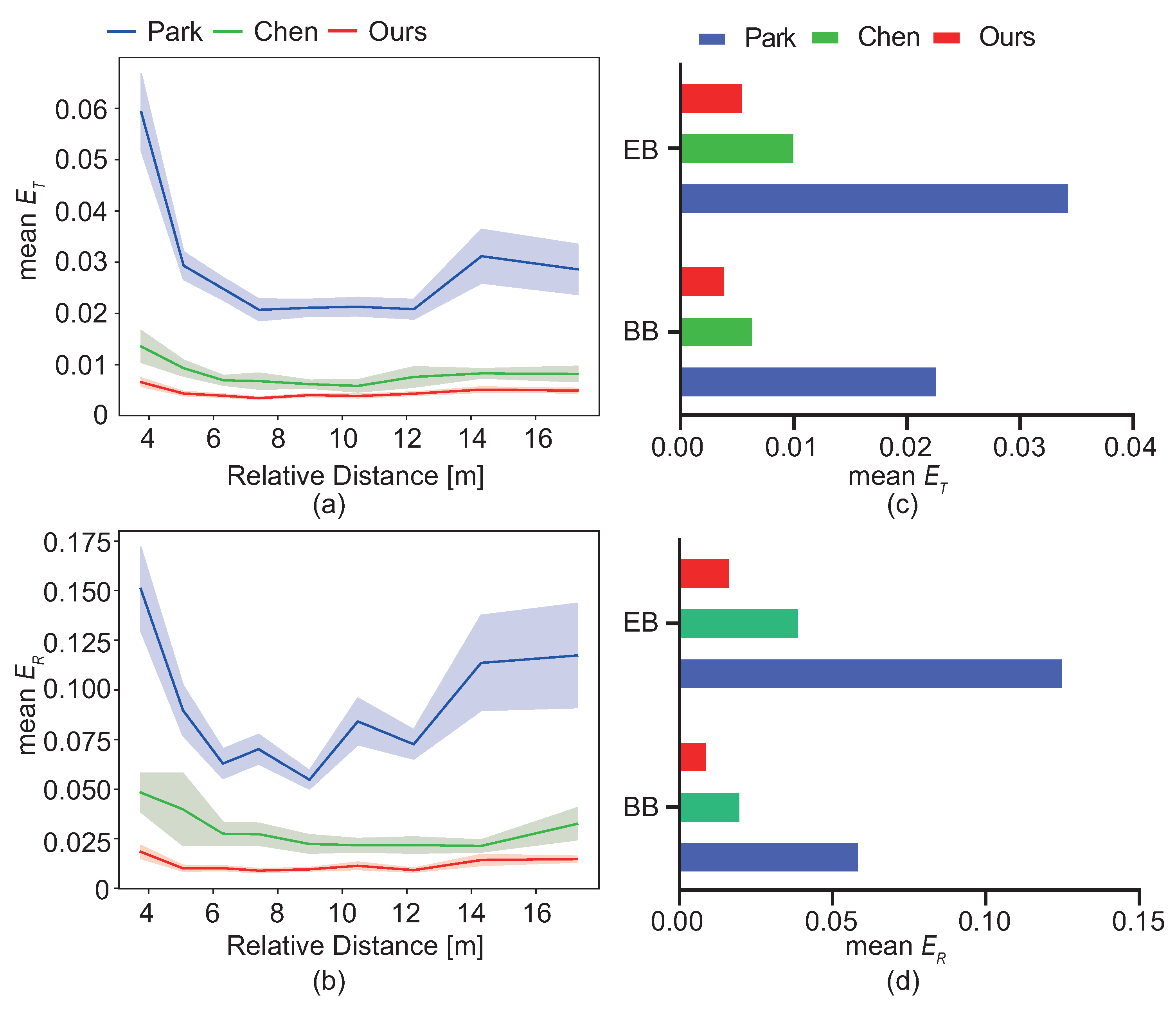
4.4. Different Conditions for Pose Estimation

4.4.1. Performance with Different Background

In this section, we compare three methods in images with different backgrounds (Figure 6c,d). Among the 1000 synthetic images, 506 have Earth backgrounds with different degrees of complexity (Figure 4). We divided the test set images into two groups with Earth backgrounds (EB) and pure black backgrounds (BB) to test the estimation errors of three methods. Figure 6c,d shows that our method achieves better pose estimation than Park [18] and Chen [19] in either EB or BB.

4.4.2. Performance in Different Relative Distance

In this section, we compare three methods in images with different relative distances to the spacecraft (Figure 6a,b). In the 1000 test images, we took 100 images as a group to divide the images of the test set into 20 groups in the order of relative distance. We draw the translation error and orientation error curves at different relative distances respectively. Figure 6a,b show that our method can maintain a very high prediction accuracy in each distance segment. Park’s [18] method has a greater estimation error in both too short and long distances. This is reasonable for when the spacecraft is very close, a part of the spacecraft often falls out of the camera’s field of view, called occlusion, a common challenge for object detection and segmentation [47]. When the spacecraft is far, its features in the image will become coarse, making it more difficult for the keypoints detection module to work well. Chen’s method [19] has good accuracy of translation estimation in each distance segment, but the error of orientation estimation is still affected by the too-long or short relative distance. Our method achieves stable translation and orientation estimation accuracy over the full range segment, proving that our method is more capable of resisting target occlusion and recovering the feature of small spacecraft.

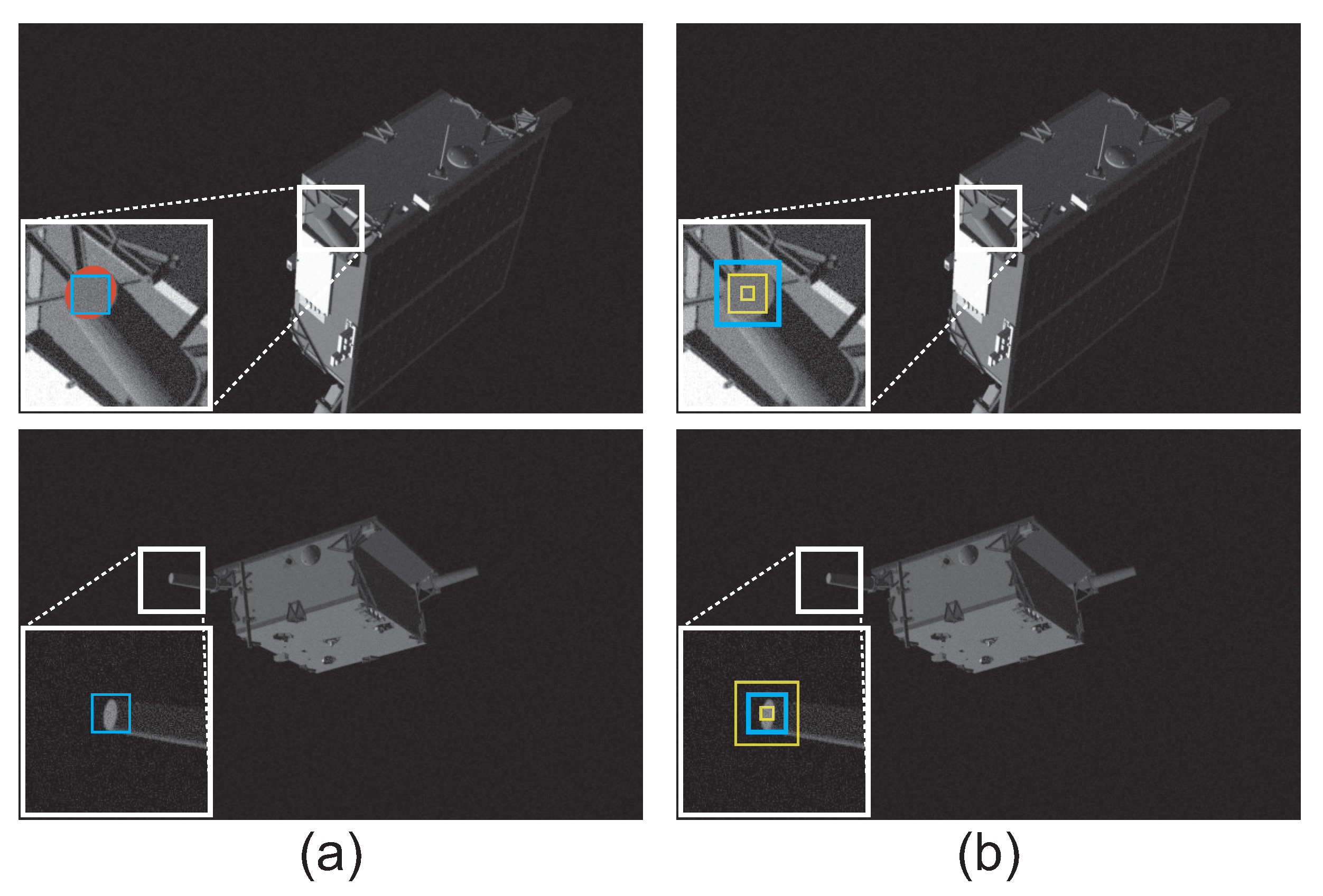
4.5. Effective Uncertainty Prediction

We conducted an ablation study to prove the effectiveness of our uncertainty prediction and keypoints selection strategy. According to Algorithm 1, we can only take UTS strategy or Top K strategy to select keypoints. If both strategies were not taken, we directly chose all eleven keypoints to estimate the pose with EPnP [24]. Here, we set $\mu$ and $K_n$ as 0.5 and 7 (Top 7) for the analysis in Section 4.7.

Table 3. Ablation study to evaluate the effectiveness of our UTS and Top 7 strategy.

Method	UTS	Top 7	${\mathit{meanE}}_{\mathit{T}}$	${\mathit{meanE}}_{\mathit{R}}$	$\mathit{meanE}$
Ours			0.0074	0.0216	0.0290
		✓	0.0056	0.0151	0.0207
	✓		0.0059	0.0179	0.0238
	✓	✓	0.0049	0.0129	0.0178

shows that both strategies can improve the accuracy of pose estimation of our method separately, and our complete keypoints selection strategy helps our method achieve the best estimation.

We show four cases that demonstrate the effectiveness of our uncertainty prediction and keypoints selection strategy in Figure 7. The lower right corner marks the percentage reduction in the three-class estimation errors after removing the detection points in red. Our selection strategy succeeded in selecting accurate keypoints with effective uncertainty prediction to reduce the error of pose estimation.

Although Chen [19] proposed an iterative trial-and-error method to remove some detected keypoints, they did not consider that this method would increase the time cost of the entire pose estimation process. Our method performs this by the uncertainty prediction of the network.

4.6. Comparison between SA and LS

In order to verify the superiority of using SA to solve the optimal problem in Equation (1), we recovered a new 3D wireframe model through LS for all the 22 images and analyzed the changes in the accuracy of the three versions of our method.

Table 4. The performance of three versions of our method on 1000 synthetic images with different 3D wireframe models from SA or Least Square LS.

Method	SA/LS	${\mathit{medianE}}_{\mathit{T}}$	${\mathit{medianE}}_{\mathit{R}}$	$\mathit{medianE}$	${\mathit{meanE}}_{\mathit{T}}$	${\mathit{meanE}}_{\mathit{R}}$	$\mathit{meanE}$
Ours	SA	0.0036	0.0073	0.0116	0.0049	0.0129	0.0178
	LS	0.0058	0.0325	0.0407	0.0083	0.0422	0.0505
Ours-small	SA	0.0041	0.0088	0.0138	0.0057	0.0235	0.0292
	LS	0.0065	0.0334	0.0419	0.0093	0.0535	0.0628
Ours-nano	SA	0.0048	0.0118	0.0175	0.0069	0.0270	0.0338
	LS	0.0070	0.0364	0.0445	0.0095	0.0541	0.0636

shows that all six error metrics for the three versions have increased when using LS to recover the wireframe model. Our SA method can help to obtain a more accurate 3D wireframe model under the noise from manual selection of images.

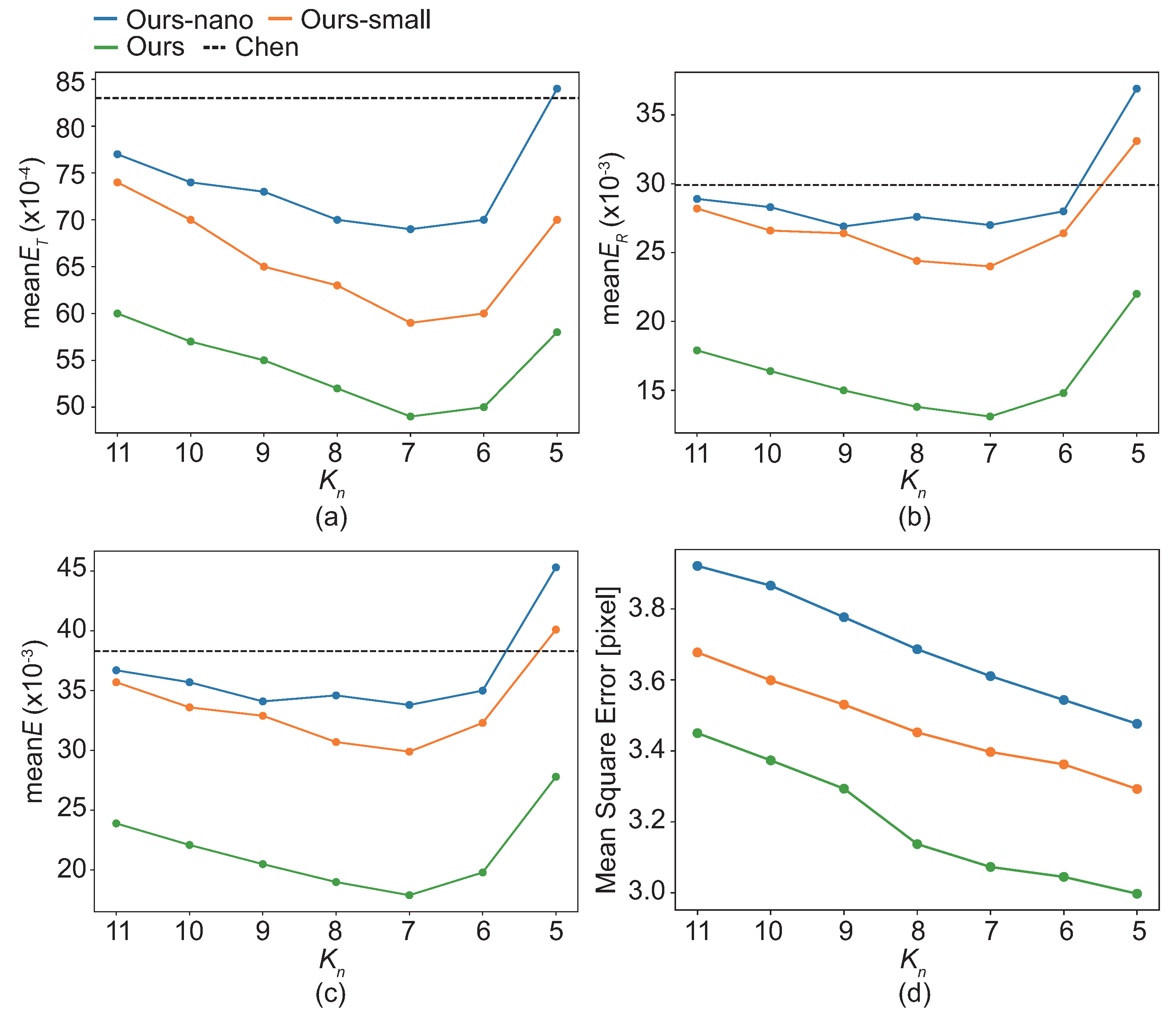
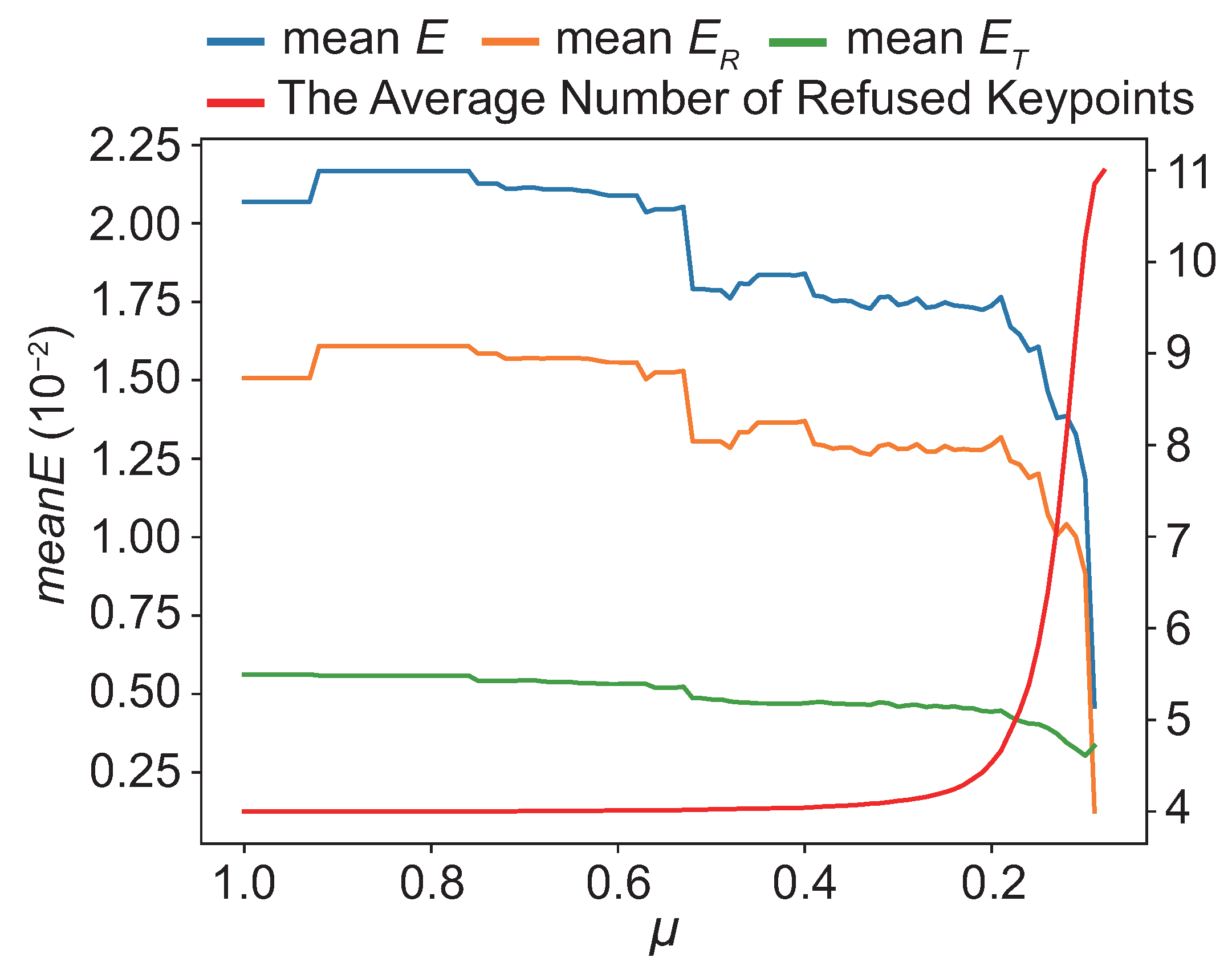
4.7. Hyperparameters Analysis

We conducted a hyperparameters analysis to study how $K_n$ and $\mu$ in Algorithm 1 affect the pose estimation of our method.

We analyzed how the choice of $K_n$ affects the performance of our method. Although the EPnP algorithm [24] only requires more than three keypoints, since our detection result may have four coplanar points, which is fatal to the EPnP algorithm, we separately analyzed the change of three estimation errors when $K_n$ changes from five to eleven (Figure 8). Here we set the $\mu$ as 0.5. All three versions of our method show the same pattern of changes. As $K_n$ changes from five to seven, the estimation error decreases gradually, which is reasonable for larger point sets to introduce redundancy and reduce the sensitivity to noise [24]. However, when $K_n$ changes from seven to eleven, the estimation errors of three versions increases. We consider that compared with the top seven keypoints, the errors introduced by the last four keypoints are too large to improve the accuracy, which also proves the validity of our uncertainty prediction.

We took our version to analyze how the $\mu$ affects the pose estimation of our method. Here, we set $K_n$ as 7, which works best. Figure 9 shows that all three errors decrease as the $\mu$ decreases, proving that the uncertainty our KDN predicts for each keypoint has a certain positive correlation with its detection error. We call the keypoints screened out by our keypoints selection strategy as refused keypoints. When the $\mu$ changes from 1.0 to 0.4, the average number of refused keypoints remains generally unchanged. When it changes to 0.2, this number begins to rise rapidly, which means that our method fails to complete the pose estimation from the corresponding images, since the number of available keypoints does not meet the acquirement of the EPnP algorithm [24]. Therefore, in practical applications, it is necessary to consider the trade-off between the continuity and accuracy of 6D pose estimation.

5. Conclusions

In this paper, we proposed a monocular pose estimation framework for space-borne objects, such as spacecraft. Our main contribution is to introduce the idea of area detection into the task of spacecraft keypoints detection and use the uncertainty of keypoints predicted by our KDN to automatically select keypoints with higher prediction accuracy to estimate the 6D pose of the spacecraft. Our method achieves a 53.3% reduction in pose estimation error with the reduction of the number of network parameters.

In future work, we will study how to adaptively choose the k value of the Top k strategy to achieve a more effective trade-off between estimation precision and computational efficiency.

References

1. Kassebom, M. Roger-an advanced solution for a geostationary service satellite. In Proceedings of the 54th International Astronautical Congress of the International Astronautical Federation, Bremen, Germany, 29 Septmber–3 October 2003; p. U-1. [Google Scholar]
2. Saleh, J.H.; Lamassoure, E.; Hastings, D.E. Space systems flexibility provided by on-orbit servicing: Part 1. J. Spacecr. Rockets 2002, 39, 551–560. [Google Scholar] [CrossRef]
3. Taylor, B.; Aglietti, G.; Fellowes, S.; Ainley, S.; Salmon, T.; Retat, I.; Burgess, C.; Hall, A.; Chabot, T.; Kanan, K.; et al. Remove debris mission, from concept to orbit. In Proceedings of the SmallSat 2018-32nd Annual AIAA/USU Conference on Small Satellites, Logan, UT, USA, 4–9 August 2018; pp. 1–10. [Google Scholar]
4. Andert, F.; Ammann, N.; Maass, B. Lidar-aided camera feature tracking and visual slam for spacecraft low-orbit navigation and planetary landing. Adv. Aerosp. Guid. Navig. Control. 2015, 605–623. [Google Scholar] [CrossRef]
5. Gaudet, B.; Furfaro, R.; Udrea, B. Attitude estimation via LIDAR altimetry and a particle filter. In Proceedings of the 24th AAS/AIAA Space Flight Mechanics Meeting, Orlando, FL, USA, 26–30 January 2014; pp. 1449–1459. [Google Scholar]
6. Axelrad, P.; Ward, L.M. Spacecraft attitude estimation using the Global Positioning System-Methodology and results for RADCAL. J. Guid. Control. Dyn. 1996, 19, 1201–1209. [Google Scholar] [CrossRef]
7. Cassinis, L.P.; Fonod, R.; Gill, E. Review of the robustness and applicability of monocular pose estimation systems for relative navigation with an uncooperative spacecraft. Prog. Aerosp. Sci. 2019, 110, 100548. [Google Scholar] [CrossRef]
8. Sharma, S.; Ventura, J. Robust Model-Based Monocular Pose Estimation for Noncooperative Spacecraft Rendezvous. J. Spacecr. Rockets 2017, 55, 1–35. [Google Scholar]
9. Dhome, M.; Richetin, M.; Lapreste, J.T. Determination of the attitude of 3D objects from a single perspective view. IEEE Trans. Pattern Anal. Mach. Intell. 1989, 11, 1265–1278. [Google Scholar] [CrossRef]
10. Kanani, K.; Petit, A.; Marchand, E.; Chabot, T.; Gerber, B. Vision based navigation for debris removal missions. In Proceedings of the 63rd International Astronautical Congress, Naples, Italy, 1–5 October 2012. [Google Scholar]
11. Petit, A.; Marchand, E.; Kanani, K. Vision-based detection and tracking for space navigation in a rendezvous context. In Proceedings of the Artificial Intelligence, Robotics and Automation in Space, Turin, Italy, 4–6 September 2012. [Google Scholar]
12. Sharma, S.; Ventura, J.; D’Amico, S. Robust model-based monocular pose initialization for noncooperative spacecraft rendezvous. J. Spacecr. Rockets 2018, 55, 1414–1429. [Google Scholar] [CrossRef] [Green Version]
13. Augenstein, S.; Rock, S.M. Improved frame-to-frame pose tracking during vision-only SLAM/SFM with a tumbling target. In Proceedings of the IEEE International Conference on Robotics and Automation, Shanghai, China, 9–13 May 2011; IEEE: London, UK, 2011; pp. 3131–3138. [Google Scholar]
14. Shi, J.; Ulrich, S.; Ruel, S. Spacecraft pose estimation using a monocular camera. In Proceedings of the 67th International Astronautical Congress, Guadalajara, Mexico, 26–30 September 2016. [Google Scholar]
15. D’Amico, S.; Benn, M.; Jørgensen, J.L. Pose estimation of an uncooperative spacecraft from actual space imagery. Int. J. Space Sci. Eng. 2014, 2, 171–189. [Google Scholar]
16. Krizhevsky, A.; Sutskever, I.; Hinton, G.E. Imagenet classification with deep convolutional neural networks. In Proceedings of the Neural Information Processing Systems, Lake Tahoe, NV, USA, 3–8 December 2012; Volume 25. [Google Scholar]
17. Sharma, S.; D’Amico, S. Pose estimation for non-cooperative rendezvous using neural networks. In Proceedings of the 29th AIAA/AAS Space Flight Mechanics Meeting, Ka’anapali, HI, USA, 13–17 January 2019. [Google Scholar]
18. Park, T.H.; Sharma, S.; D’Amico, S. Towards Robust Learning-Based Pose Estimation of Noncooperative Spacecraft. In Proceedings of the AAS/AIAA Astrodynamics Specialist Conference, Portland, ME, USA, 11–15 August 2019. [Google Scholar]
19. Chen, B.; Cao, J.; Parra, A.; Chin, T.J. Satellite pose estimation with deep landmark regression and nonlinear pose refinement. In Proceedings of the IEEE/CVF International Conference on Computer Vision Workshops, Seoul, Korea, 27 October–2 November 2019. [Google Scholar]
20. Park, T.H.; D’Amico, S. Robust Multi-Task Learning and Online Refinement for Spacecraft Pose Estimation across Domain Gap. In Proceedings of the the 11th International Workshop on Satellite Constellations & Formation Flying, Milan, Italy, 7–10 June 2022. [Google Scholar]
21. Proença, P.F.; Gao, Y. Deep learning for spacecraft pose estimation from photorealistic rendering. In Proceedings of the 2020 IEEE International Conference on Robotics and Automation, Online, 31 May 2020; IEEE: New York, NY, USA, 2020; pp. 6007–6013. [Google Scholar]
22. Sharma, S.; Beierle, C.; D’Amico, S. Pose estimation for non-cooperative spacecraft rendezvous using convolutional neural networks. In Proceedings of the IEEE Aerospace Conference, Big Sky, MT, USA, 4–11 March 2019; IEEE: New York, NY, USA, 2018; pp. 1–12. [Google Scholar]
23. Sharma, S.; D’Amico, S. Neural network-based pose estimation for noncooperative spacecraft rendezvous. IEEE Trans. Aerosp. Electron. Syst. 2020, 56, 4638–4658. [Google Scholar] [CrossRef]
24. Lepetit, V.; Moreno-Noguer, F.; Fua, P. Epnp: An accurate o (n) solution to the pnp problem. Int. J. Comput. Vis. 2009, 81, 155–166. [Google Scholar] [CrossRef] [Green Version]
25. Sandler, M.; Howard, A.; Zhu, M.; Zhmoginov, A.; Chen, L.C. Mobilenetv2: Inverted residuals and linear bottlenecks. In Proceedings of the the IEEE/CVF Conference on Computer Vision and Pattern Recognition, Salt Lake City, UT, USA, 18–23 June 2018; pp. 4510–4520. [Google Scholar]
26. Long, J.; Shelhamer, E.; Darrell, T. Fully convolutional networks for semantic segmentation. In Proceedings of the IEEE/CVF Conference on Computer Vision and Pattern Recognition, Boston, MA, USA, 7–12 June 2015; pp. 3431–3440. [Google Scholar]
27. Lenc, K.; Vedaldi, A. Large scale evaluation of local image feature detectors on homography datasets. In Proceedings of the 29th British Machine Vision Conference, Newcastle, UK, 3–6 September 2018. [Google Scholar]
28. Harris, C.; Stephens, M. A combined corner and edge detector. In Proceedings of the Alvey Vision Conference, Manchester, UK, 31 August–2 September 1988; Volume 15, pp. 147–151. [Google Scholar]
29. Beaudet, P.R. Rotationally invariant image operators. In Proceedings of the 4th International Joint Conference Pattern Recognition, Kyoto, Japan, 7–10 November 1978. [Google Scholar]
30. Lowe, D.G. Distinctive image features from scale-invariant keypoints. Int. J. Comput. Vis. 2004, 60, 91–110. [Google Scholar] [CrossRef]
31. Rublee, E.; Rabaud, V.; Konolige, K.; Bradski, G. ORB: An efficient alternative to SIFT or SURF. In Proceedings of the 2011 International Conference on Computer Vision, Barcelona, Spain, 6–13 November 2011; IEEE: New York, NY, USA, 2011; pp. 2564–2571. [Google Scholar]
32. Matas, J.; Chum, O.; Urban, M.; Pajdla, T. Robust wide-baseline stereo from maximally stable extremal regions. Image. Vis. Comput. 2004, 22, 761–767. [Google Scholar] [CrossRef]
33. Bay, H.; Tuytelaars, T.; Gool, L.V. Surf: Speeded up robust features. In Proceedings of the European Conference on Computer Vision, Graz, Austria, 7–13 May 2006; Springer: Berlin/Heidelberg, Germany, 2006; pp. 404–417. [Google Scholar]
34. Rosten, E.; Drummond, T. Machine learning for high-speed corner detection. In Proceedings of the European Conference on Computer Vision, Graz, Austria, 7–13 May 2006; Springer: Berlin/Heidelberg, Germany, 2006; pp. 430–443. [Google Scholar]
35. Rosten, E.; Porter, R.; Drummond, T. Faster and better: A machine learning approach to corner detection. IEEE Trans. Pattern Anal. Mach. Intell. 2008, 32, 105–119. [Google Scholar] [CrossRef] [PubMed] [Green Version]
36. Leutenegger, S.; Chli, M.; Siegwart, R.Y. BRISK: Binary robust invariant scalable keypoints. In Proceedings of the 2011 International Conference on Computer Vision, Barcelona, Spain, 6–13 November 2011; pp. 2548–2555. [Google Scholar]
37. Verdie, Y.; Yi, K.; Fua, P.; Lepetit, V. Tilde: A temporally invariant learned detector. In Proceedings of the IEEE Conference on Computer Vision and Pattern Recognition, Boston, MA, USA, 7–12 June 2015; pp. 5279–5288. [Google Scholar]
38. Georgakis, G.; Karanam, S.; Wu, Z.; Ernst, J.; Košecká, J. End-to-end learning of keypoint detector and descriptor for pose invariant 3D matching. In Proceedings of the IEEE/CVF Conference on Computer Vision and Pattern Recognition, Salt Lake City, UT, USA, 18–23 June 2018; pp. 1965–1973. [Google Scholar]
39. Ono, Y.; Trulls, E.; Fua, P.; Yi, K.M. LF-Net: Learning local features from images. NeurIPS 2018, 31, 6234–6244. [Google Scholar]
40. Sun, K.; Xiao, B.; Liu, D.; Wang, J. Deep high-resolution representation learning for human pose estimation. In Proceedings of the IEEE/CVF Conference on Computer Vision and Pattern Recognition, Long Beach, CA, USA, 15–20 June 2019; pp. 5693–5703. [Google Scholar]
41. Xiang, Y.; Gubian, S.; Suomela, B.; Hoeng, J. Generalized simulated annealing for global optimization: The GenSA package. R J. 2013, 5, 13. [Google Scholar] [CrossRef]
42. Ge, Z.; Liu, S.; Wang, F.; Li, Z.; Sun, J. Yolox: Exceeding yolo series in 2021. arXiv 2021, arXiv:2107.08430. [Google Scholar]
43. Bochkovskiy, A.; Wang, C.Y.; Liao, H.Y.M. Yolov4: Optimal speed and accuracy of object detection. arXiv 2020, arXiv:2004.10934. [Google Scholar]
44. Lin, T.Y.; Dollár, P.; Girshick, R.; He, K.; Hariharan, B.; Belongie, S. Feature pyramid networks for object detection. In Proceedings of the IEEE Conference on Computer Vision and Pattern Recognition, Honolulu, HI, USA, 21–26 July 2017; pp. 1–13. [Google Scholar]
45. Kelvins Pose Estimation Challenge 2019. Available online: https://kelvins.esa.int/satellite-pose-estimation-challenge/ (accessed on 4 July 2022).
46. Kelvins Pose Estimation Challenge 2021. Available online: https://kelvins.esa.int/pose-estimation-2021/challenge/ (accessed on 14 July 2022).
47. Gao, T.; Packer, B.; Koller, D. A segmentation-aware object detection model with occlusion handling. In Proceedings of the 24th IEEE Conference on Computer Vision and Pattern Recognition, Colorado Springs, CO, USA, 20–25 June 2011; pp. 1361–1368. [Google Scholar]
Figure 1. Our advantage over Chen [19] on how to set the region of keypoints. (a) Chen [19], (b) Ours. The blue box represents the box containing a keypoint, and the yellow box represents the anchor in our Keypoint Detection Network. When the relative distance of the spacecraft is too small, the fixed region ignores some key area of the keypoint. However, our adaptive region size can solve this problem better, which is described in Section 2.2.
Aerospace 09 00592 g001
Figure 2. The pipeline of our proposed method to estimate the 6D pose of a spacecraft from a monocular image. SDN: Spacecraft Detection Network. KDN: Keypoint Detection Network. SA: Simulated Annealing.
Aerospace 09 00592 g002
Figure 3. The framework of our KDN.
Aerospace 09 00592 g003
Figure 4. Images with Different Conditions in 12,000 Synthetic Images. They vary in light intensity, relative distance to spacecraft, perspective and background complexity.
Aerospace 09 00592 g004
Figure 5. Pose Estimation Performance in five real images. (a) Ours, (b) Park [18], (c) Chen [19].
Aerospace 09 00592 g005
Figure 6. Performance in Different Relative Distance and Background. (a,b) show the change of m e a n E T and m e a n E R respectively with the relative distance between the spacecraft and the camera. (c,d) show the change of m e a n E T and m e a n E R respectively with the different backgrounds. EB represents the 506 images with the earth background in the test set, as shown in the bottom row in Figure 7. BB represents the 494 images with black background in the test set, as shown in the top row in Figure 7.
Aerospace 09 00592 g006
Figure 7. Uncertainty Prediction Helps Reduce Pose Estimation Error. The blue points represent the key points that we retained for pose estimation, the red points represent the key points that we eliminated due to the high uncertainty, the yellow points represent the true positions of the eliminated keypoints, and we used the green dotted line Connect the corresponding yellow and red points.
Aerospace 09 00592 g007
Figure 8. Performance with different K n . (ac) show the change of three kinds of error with the selection of K n . (d) shows the change of MSE error of detected keypoints with the selection of K n .
Aerospace 09 00592 g008
Figure 9. The m e a n E and Number of Refused Images with Different μ .
Aerospace 09 00592 g009