Hopf Bifurcation Analysis of the Combustion Instability in a Liquid Rocket Engine

Abstract

The bifurcation process of self-sustained combustion instability pressure perturbations in a liquid rocket combustor is investigated based on the Helmholtz equations and a pressure dependent flame describing function. The modal frequency and growth rates are numerically resolved by the commercial software COMSOL multiphysics. Validation of the numerical approach is firstly conducted on a Rijke tube combustor, and a supercritical bifurcation for the first longitudinal mode is observed. The bifurcation diagrams for the first transverse mode for different time delays and gain index of the flame describing function are analyzed. Only the supercritical bifurcation presents for this configuration. The trajectory of Hopf points and the bifurcation diagram feature period motions with increasing the time delay. The effect of flame length distributions on the bifurcation diagrams is analyzed by considering a non-uniform flame length distribution model. Results show that the distribution has a large impact on the bifurcation process, e.g., the first transverse mode is more unstable for the non-uniform distribution. Finally, a subcritical bifurcation is found when a more complicated flame describing function is considered; the bistable region presents and the condition for this is discussed.

1. Introduction

Combustion instability (CI) has been considered as one of the most difficult and challenging problems in aeronautics [1], astronautics [2,3] and other burners. Due to the severe operating conditions in the combustion chamber (high temperature, extremely high pressure and large energy density), CI more easily to occurs in liquid rocket engines (LRE) [4]. CI may lead to severe pressure oscillation in the combustion chamber, resulting in damages to injectors, the combustion chamber or other components and even causing an explosion. However, due to the highly complex multi-process coupling among injecting, vaporizing, combustion, acoustic characteristic, boundary condition and other factors, it is still much difficult to predict and eliminate the CI [5,6,7,8,9].

In 1859, Rijke found that unstable acoustic oscillations occured when the heat source was placed in a vertical tube, which provided a simple configuration to study the complicated CI phenomenon [10]. Based on the Rijke tube, many complex CI phenomena presenting in real geometries could be reproduced [11,12,13]. These studies could be extended to more complicated models by thoughtful deduction and appropriate extension [12,14,15]. Sujith et al. investigated the non-normality and nonlinearity in the CI interaction in a Rijke tube [16]. Bifurcation conduct has been identified in Rijke tube experimentally [17,18]. An online monitoring and optimization algorithm was developed based on the least mean square method to mitigate the CI in a Rijke tube [19,20]. Although these simplified models have captured the major features of the CI and facilitate the understanding of CI [11,21], the structure of it is relatively simple compared to full-scale combustion devices. At the same time, the flow in Rijke tubes is essentially regarded as laminar condition, which would not be sufficient to explain the dynamics of practical combustors with turbulent flow. Moreover, since only longitudinal modes are suited for studying in Rijke tubes, they still cannot reveal more factors of the true combustion chambers.

The BKD model combustor, which is a reduced-scale rocket engine developed at the DLR Lampoldshausen, has been considered as a benchmark test rig for the investigations of LRE combustion instabilities, and a great many researches have been conducted based on this configuration [22,23,24]. The linearized Euler code PIANO considering the mean flow and response function was applied to perform a complete stability analysis [25]. Gröning et al. [26] analysed the effect of hydrogen temperature on the high frequency CI in the BKD combustor. The compressible LES study of self sustained transversal CI and flame response subjected to transversal perturbations in the BKD were carried out by Urbano and her colleagues [27,28], and more practical results, e.g., mode triggering, were obtained. Machine learning has been applied for thermoacoustic instabilities in the BKD combustor, performance evaluated [29].

Due to the nonlinear responses of the flame and even the acoustic waves (these typically only occur in rocket engines), the CI features more complex behaviours. During past several decades, many researches have been conducted to develop linear and nonlinear theories [30,31,32,33]. Linear analysis is simple but is limited. Only linear stability can be obtained according to the linear analysis, and temporary status and the developing process of fluctuation typically cannot be determined [12]. Dowling has developed and summarized the low order models for the predictions of the CI in a simple duct combustor [11] and annular combustion chambers [14]. In order to capture the mode triggering and the limit cycle characteristics of the CI, nonlinear analysis is needed and a great many researches have been conducted to develop the nonlinear theories. Lieuwen studied the limit cycle phenomenon in a gas turbine combustor experimentally [34]. A typical self-exited CI of lean premixed combustion was examined by Sun [35], and the nonlinear bifurcation was captured. A comprehensive nonlinear combustion instability model has been proposed by Flandro [36]. In order to obtain the bifurcation diagram, systematic variation of parameters and tracking direct time integration were conducted by [37,38]. Besides, the nonlinear behavior of the solid rocket motor was analyzed to investigate the bistable region for the different responses [39].

As in many combustors, the flame is the major source of nonlinearity. Thus many researches have been conducted to develop the nonlinear flame response model, and it is also called the flame describing function (FDF) for the weakly nonlinear analysis. A lot of researches have worked out the nonlinear flame response for certain simple flames, e.g., the laminar premixed conical flame, based on the G-equation model [33,40,41,42,43,44]. These models reveal the nonlinear dynamic flame responses and are much closer to real flames. However, they are limited to simple flame geometries, and are not suitable for highly complex turbulent flames. In the Rijke tube fed by a hot wire, the King’s law is widely used to relate the nonlinear heat and the oncoming flow velocities, and this model has been coupled in the Galerkin theory to capture the nonlinear properties and even the subcritical and supercritical bifurcation [45]. The heat source of course can also be replaced by a laminar premixed conical flame model based on the G-equation method, and the results are more meaningful to the combustion research [13,46].

Other researches try to put forward simple nonlinear models which capture the main features of flame subjected to oncoming disturbances. Dowling has proposed a saturation model of the normalised heat release rate based on the fact that the heat release rate perturbation cannot be larger than the time-averaged heat release rate [31]. This model has been successfully used to capture the nonlinear interaction between longitudinal modes and circumferential modes in an annular combustion chamber [47], and has been further used to capture the nonlinear saturation in a Rijke tube combustor [48]. Li and Morgans had improved this model, considering a nonlinear factor contributing to both amplitude and phase of the FDF, and applied it to reconstruct different nonlinear CI behaviours in a Rijke tube [12]. Other researchers established polynomial relations between the heat release rate disturbance and oncoming perturbation, which is much easier to be used in the low order time domain simulation scheme [49,50]. Noiray has coupled a three order flame response model as a function of the pressure perturbation into a Galerkin approach to analyse the nonlinear circumferential mode in gas turbines [49]. Campa and Juniper have coupled the three orders and five orders flame models in the low order network code—LOTAN, to simulate the nonlinear bifurcations [51]. The nature of the Hopf bifurcation was analysed for different nonlinear flame models. These two models have been further coupled in the Helmholtz equations to simulate the nonlinear CI in more complex geometries [52,53], which used the usual velocity dependent flame transfer function. As for most combustors, the major nonlinearities come from the nonlinear flame responses; this facilitates the analysis of combustion instabilities based on the Helmholtz equation, with the nonlinear flame response as the source.

The objective of the present work is to couple the nonlinear polynomial pressure dependent flame describing function into a Helmholtz equation model of the BKD combustor to study the Hopf bifurcation of combustion instability in the LRE. The combustion instability in a Rijke tube was studied firstly and then that of the BKD combustor with different distributed flame lengths. The remainder of the paper is organized as follows. The simulation models, geometry models (Rijke tube and BKD combustor), nonlinear flame model and distributed flame lengths model are introduced in Section 2. The nonlinear analysis method was introduced in Section 3. Section 4 presents the results and the discussion of the bifurcation diagram. Finally, the conclusion is shown in Section 5.

2. Simulation Models

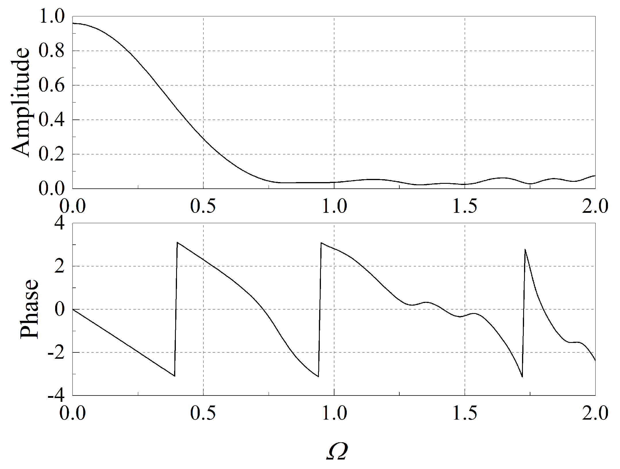
2.1. Governing Equations and the Model of Flame Describing Function

The fluid in the target combustion chamber is considered as ideal gas. The effects of viscosity, heat diffusion and heat conduction can be neglected. The pressure and the velocity within the chamber are supposed to be uniform. Because the mean flow velocity is far smaller than the speed of sound, it is reasonable to assume a zero mean flow, even for LRE combustor [54,55]. Under these assumptions and the small perturbation assumption, it is easy to get the inhomogeneous wave equation as a function of the pressure perturbation $p^{\prime }$ [11,14]:

$$\frac{1}{{\overline{c}}^2}\frac{{\partial }^2{p}^{\prime }}{\partial t^2}-\overline{\rho }\nabla ·(\frac{1}{\overline{\rho }}\nabla p^{\prime })=\frac{(\gamma -1)}{{\overline{c}}^2}\frac{\partial q^{\prime }}{\partial t}$$

(1)

where q represents the heat release rate per unit volume and c is the speed of sound. $\rho$ and $\gamma$ denote the density and the specific heat ratio, respectively. $\overline{\left(\right)}$ means an average value and ${\left(\right)}^{\prime }$ indicates a perturbation value. With the assumption of perturbations on the basic frequency, $a^{\prime }\left(t\right)=\widehat{\mathit{a}}exp\left(\mathrm{i}\omega t\right)$, where a could be p or q. $\omega$ is the complex angular frequency; its real part $\mathcal{R}\left(\omega \right)=2\pi f$ represents the angular frequency, and its imaginary part $\mathcal{I}\left(\omega \right)=-\alpha$ corresponds to the modal growth rate. When $\alpha >0$, the acoustic mode is unstable, and the disturbances grow with time. When $\alpha <0$, the acoustic mode is stable, and the disturbances decay with time. When $\alpha =0$, the acoustic mode is marginal stable or a limit cycle for a perturbation is established. By substituting the above expression into it, the wave equation can be changed to the expression in the frequency domain:

$$\frac{{\omega }^2}{{\overline{c}}^2}\widehat{p}+\overline{\rho }\nabla ·(\frac{1}{\overline{\rho }}\nabla \widehat{p})=-\frac{(\gamma -1)}{{\overline{c}}^2}\mathrm{i}\omega \widehat{q}.$$

(2)

A finite element method (FEM) based the commercial software COMSOL multiphysics is used to solve the Helmholtz equation. This numerical scheme is based on the ARPACK numerical routine for large-scale eigenvalue problems [56]. The numerical procedure is iterated until the error is smaller than ${10}^{-4}$ Hz. In previous researches, the flame response to oncoming disturbances is typically based on the relation between the heat release rate and the axial flow velocity perturbations [53]. However, in the rocket combustion chamber, transverse CI typically occurs and the model based on the axial velocity perturbation is limited. One thus prefers the flame response model to local pressure perturbations.

In order to account for the nonlinearity of the heat release rate, a flame response model adopted the classical $n-\tau$ model [57] and the nonlinearity is introduced by a third order term as used in [51,53], and this model can be expressed in the time domain as:

$$\frac{q^{\prime }\left(t\right)}{\overline{q}}=-n\left(\left(\frac{p^{\prime }\left(t\right)}{\overline{p}}-\frac{p^{\prime }(t-\tau )}{\overline{p}}\right)-\mu {\left(\frac{p^{\prime }\left(t\right)}{\overline{p}}-\frac{p^{\prime }(t-\tau )}{\overline{p}}\right)}^3\right)$$

(3)

where n and $\tau$ are the gain index and the time delay of the $n-\tau$ model, respectively. It is noted that the presence of the third order term leads to the nonlinear flame response. $\mu$ is a coefficient related to the strength of the third order term compared the first order term. In the present paper, the coefficient $\mu$ equals 2 for the nonlinear analyses and equals 0 for the linear analyses. In order to couple the flame response model in the frequency domain analysis, a weakly nonlinear flame model, also called the FDF, can be obtained by accounting for the Laplace transform of the fundamental term of heat release rate perturbation from Equation (3), and the FDF can be expressed as:

$$F(\omega ,\beta )=\frac{\widehat{q}/\overline{q}}{\widehat{p}/\overline{p}}=-n\left(1-e^{-\mathrm{i}\omega \tau }\right)\left(1-\frac{3\mu }{4}{\beta }^2\right)$$

(4)

where $\beta =|\widehat{p}/\overline{p}|$. It is noted that, when normalised pressure perturbation amplitude $\beta$ remains small, the third order term is much smaller than the first order term, and the flame describing function becomes a linear relation; with increasing $\beta$, the gain of the flame describing function obviously decreases, that captures the saturation behaviour of the flame dynamic response [58]. As the time delays in the first order and the third order terms are the same, the gain of the FDF decreases monotonously [50].

The nonlinearity term of a fifth order polynomial was similarly introduced,

$$\frac{q^{\prime }\left(t\right)}{\overline{q}}=-n\left(\left(\frac{p^{\prime }\left(t\right)}{\overline{p}}-\frac{p^{\prime }(t-\tau )}{\overline{p}}\right)-{\mu }_3{\left(\frac{p^{\prime }\left(t\right)}{\overline{p}}-\frac{p^{\prime }(t-\tau )}{\overline{p}}\right)}^3-{\mu }_5{\left(\frac{p^{\prime }\left(t\right)}{\overline{p}}-\frac{p^{\prime }(t-\tau )}{\overline{p}}\right)}^5\right)$$

(5)

where ${\mu }_3$ and ${\mu }_5$ are the strength of the third order term and the fifth order compared to the first order term, respectively. In the present paper, the coefficient of the third order ${\mu }_3$ equals −5 and the coefficient of the fifth order 6. The corresponding FDF was obtained according to the procedure of the third FDF:

$$F(\omega ,\beta )=\frac{\widehat{q}/\overline{q}}{\widehat{p}/\overline{p}}=-n\left(1-e^{-\mathrm{i}\omega \tau }\right)\left(1-\frac{3{\mu }_3}{4}{\beta }^2-\frac{5{\mu }_5}{8}{\beta }^4\right)$$

(6)

at the moment, the amplitude of the pressure disturbance increases with the disturbance developing, resulting in the non-monotonic change of the nonlinear term, which causes more complicated nonlinear conduct.

By substituting Equations (4) and (6) into the Helmholtz Equation (2), one gets ODE equations as purely functions of $\widehat{p}$, and this equation thus can now be numerically solved.

2.2. Rijke Tube Model Combustor

Following previous research [53], the proposed models and solver have been firstly applied to the simplest geometry—Rijke tube model combustor, as shown in Figure 1. The length of the tube is 3 m and the radius of the tube is 0.1 m. Both ends of the tube considered open to the atmosphere, i.e., $p^{\prime }=0$. The flame is placed at one quarter of the tube (as represented by the red block in Figure 1), and has a width of 0.02 m. The mean temperature before and after the flame are ${\overline{t}}_1=300$ K and ${\overline{t}}_2=700$ K, respectively. The flow in the two sections is assumed as air, and the thermal properties of air are used in the calculation. The specific ratio is assumed constant and equals $\gamma =1.4$. Figure 1 also shows the mesh for the simulation.

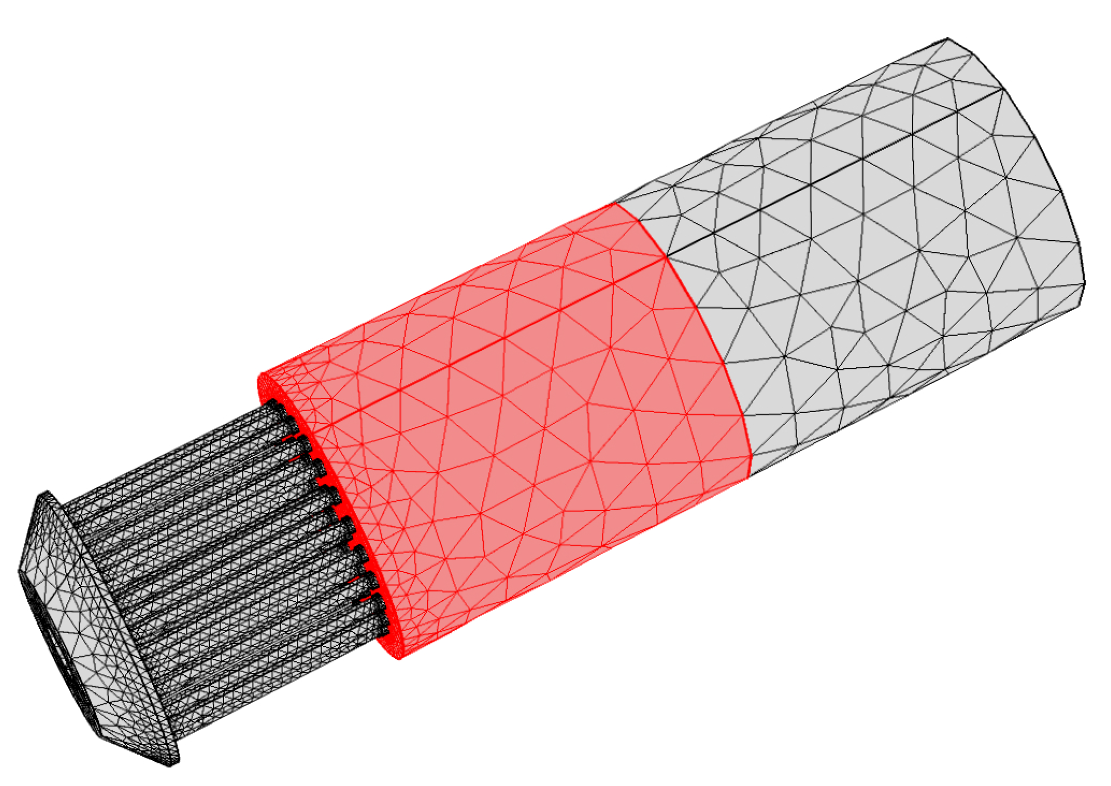
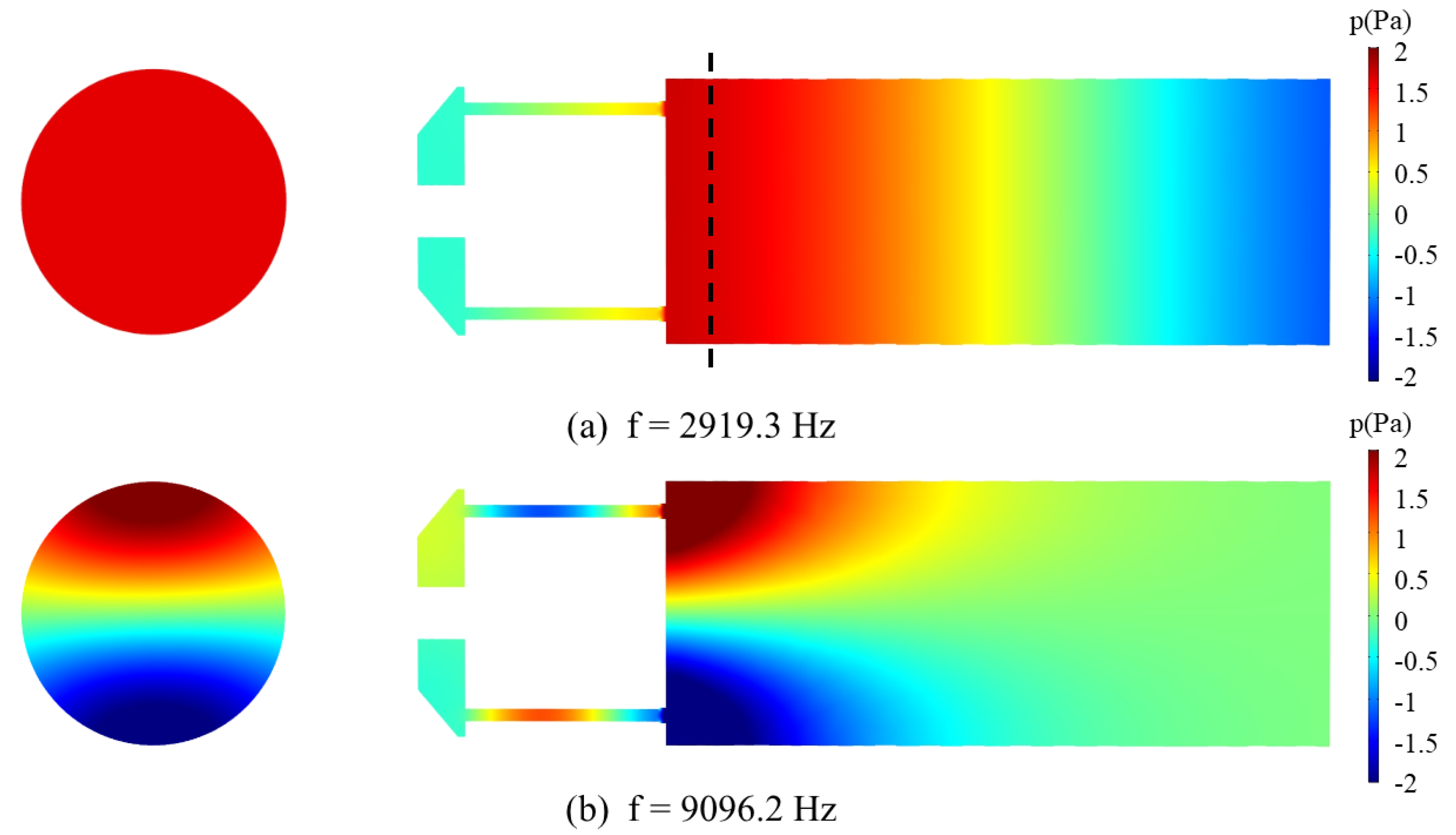
2.3. BKD Combustor Model

Further analyses are conducted on the reduced-scale rocket engine model BKD combustor. The combustion chamber of BKD is 8 cm in diameter and 20 cm in length, fed by 42 injectors. There is an injection system before the chamber and a convergent-divergent nozzle after. More parameters are described in [59]. The first transverse (1T) mode showed an unstable mode of this combustor under case LP4, presented in [60]. The pressure of combustion chamber is 80.04 bar. The operation parameters are shown as

Table 1. Operation parameter of case LP4.

	${\dot{\mathit{m}}}_{{\mathbf{H}}_2}$ (kg/s)	${\dot{\mathit{m}}}_{{\mathbf{O}}_2}$ (kg/s)	ROF (-)	${\mathit{u}}_{{\mathbf{H}}_2,\mathbf{inj}}$ (m/s)	${\mathit{u}}_{{\mathbf{O}}_2,\mathbf{inj}}$ (m/s)	${\overline{\mathit{p}}}_{\mathbf{cc}}$ (bar)
LP4	0.96	5.75	6	330	12.76	80.04

in terms of propellant mass flow rates ${\dot{m}}_{{\mathrm{O}}_2/{\mathrm{H}}_2}$, ratio of oxidizer to fuel mass flow (ROF $={\dot{m}}_{{\mathrm{O}}_2}/{\dot{m}}_{{\mathrm{H}}_2}$), velocity at injector exit $u_{{\mathrm{O}}_2/{\mathrm{H}}_2,\mathrm{inj}}$ and the average pressure of the combustion chamber ${\overline{p}}_{\mathrm{cc}}$.

The acoustic model of BKD is built upon its real geometry, whose main body is a cylinder. The FEM model is presented in Figure 2. Walls of the injectors and combustion chamber are treated as rigid walls. Hydrogen tubes were modeled by the impedance proposed by Urbano [27] ($Z=-1.160-\mathrm{i}0.255$ for the first order transverse mode) instead of modeling true hydrogen tubes to simplify the simulation. For the same purpose, the nozzle is replaced by an acoustic boundary condition, whose pressure reflection coefficient was calculated by the Magnus expansion of the governing linearised Euler equations of the nozzle [61,62]. The resulting acoustic reflection coefficient is shown in Figure 3, where $\Omega$ means the reduced frequency and $\Omega =f{L}_{\mathrm{n}}/c_0$, $L_{\mathrm{n}}$ is the nozzle length, $c_0$ is the speed of sound at the inlet of the nozzle. It is obvious that the reflection coefficient features the shape of a low pass filter. It is noted that the mean properties vary along the combustion chamber. In order to resolve the Helmholtz equation (Equation (2)), the mean properties, especially $\overline{\rho }$ and $\overline{c}$, are obtained by a RANS (Reynolds Average Navier-Stokes) of a single injector connected to a combustion chamber with an equivalent radius [63]. Figure 4 shows the mean properties along the axis from RANS and thermal calculation software REFPROP considering the supercritical state. The mean temperature arises with increasing the axial location and reaches around 3000 K when $x=0.2$ m. The mean speed of sound also increases along the combustion chamber. Due to the presence of hydrogen, the speed of sound exceeds 1500 m/s when $x=0.2$ m. Based on the numerical simulation results [27], the flame region is assumed to be extended to the half of the combustion chamber to construct the combustor model and is represented by the red block in Figure 2. Furthermore, in order to study the effect of the distribution of flame length along the radius direction on the CI, three kinds of flame length distributions are accounted for, and are presented in the following section.

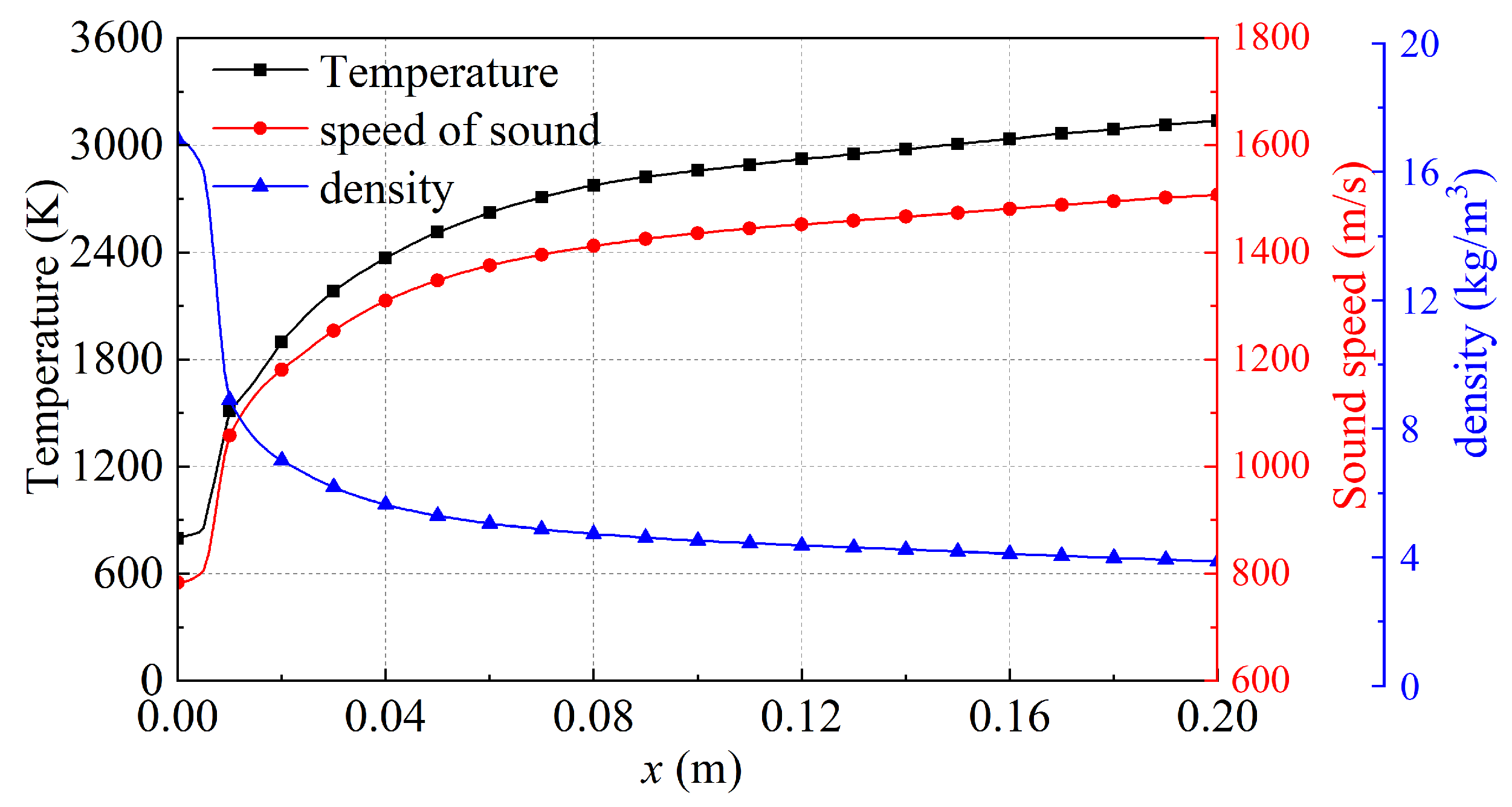
2.4. Models of Flame Distribution in the BKD Combustor

However, in the true liquid rocket engine, the flame distribution is usually not a standard cylinder, e.g., the simulation results of the BKD combustor as shown in Figure 11b in [27]. Previous researches [64,65] about real liquid rocket engines also showed that the flame region (or high temperature region) in the combustion chamber was distributed along the radius direction. One thus also accounts for another two flame distribution models, a convex shape and a concave shape. The variation of flame length along the radius obeys a Gaussian distribution, and the flame length distributions for these two models can be expressed as:

$$\frac{L_{f,\pm }\left(r\right)}{L_{\mathrm{cc}}}=\frac{1}{2}\pm \left(a\frac{1}{\sqrt{2\pi }\sigma }{e}^{-\frac{{(r/R)}^2}{2{\sigma }^2}}+b\right)$$

(7)

where $L_{f,+}\left(r\right)$ and $L_{f,-}\left(r\right)$ represent the flame lengths as a function of radius r for the convex and concave shapes, respectively. $L_{\mathrm{cc}}$ represents the length of the entire combustion chamber. $\sigma$ equals 1.58 herein, a and b equal 5.7737 and 1.1934, respectively. The difference between the flame length at the center $r=0$ and that near the lateral wall $r=R$ is 0.05 m. The uniform flame in the BKD combustor is considered half of the length of the combustion chamber, as shown in Figure 2. The flame length distribution for the three types of envisaged flames are shown as Figure 5. The variables are nondimensionalized to describe the shape of the heat resource. The effect of flame length distribution on the nonlinear CI will be described in details in Section 4.3.

3. Nonlinear Analysis

The objective of this work is to investigate the Hopf bifurcation of thermoacoustic mode when gradually increasing or decreasing a parameter, e.g., the index n, of the flame describing function. This can be achieved by looking into the growth rate $\alpha$ path of the envisaged mode with increasing the normalised pressure perturbation amplitude $\beta$ for a given value of n for instance [53]. By searching the value that $\alpha =0$, one can get the normalised pressure perturbation amplitude ${\beta }^{*}$ when the limit cycle is established. It should be noted that, for certain values of n, the system remains stable for all $\beta$, and one assigns 0 to ${\beta }^{*}$. It is then possible to consider the value of n when ${\beta }^{*}$ changes from 0 to a positive value as the Hopf point or stability margin, which means that the system changes from linear stable to unstable. The bifurcation diagram can then be established by plotting ${\beta }^{*}$ versus n. Note that the above procedure can be simplified as the gain of FDF decreases monotonously with increasing $\beta$. The mode thus is typically mostly unstable when $\beta =0$. Thus, one can firstly calculate the linear stability for all n and search the Hopf point when the modal growth rate $\alpha =0$. Considering more complex FDF, e.g., the fifth order FDF as used in [53], more complex nonlinear combustion instability behaviours, e.g., the hysteresis phenomenon, occur with increasing $\beta$. The bifurcation diagram should be constructed by carefully scanning the combustion instability properties for all n and $\beta$. In order to get the return path of the bifurcation diagram, the decreasing process of n should be conducted.

4. Results and Discussion

4.1. Rijke Tube

To get the eigenfrequency of Rijke tube, the Helmholtz equation was solved by the commercial software COMSOL Multiphysics. It should be noted that the heat release rate q in the FDF equation (Equation (4)) is the local value. The local mean heat release rate equals $\overline{q}=\overline{Q}/V_{\mathrm{f}}$, where $\overline{Q}$ and $V_{\mathrm{f}}$ are the entire mean heat release rate and the volume of the flame. For the Rijke tube, $\overline{Q}={\overline{\rho }}_1{\overline{u}}_1{c}_p({\overline{t}}_2-{\overline{t}}_1)=\gamma {\overline{u}}_1/(\gamma -1){\overline{p}}_1({\overline{t}}_2/{\overline{t}}_1-1)$, where $\overline{t}$, ${\overline{\rho }}_1$, ${\overline{u}}_1$ and $c_p$ are the mean temperature, mean flow density, velocity and heat capacity at constant pressure, respectively. It is assumed a low Mach number flow in the Rijke tube and the inlet mean flow velocity equals ${\overline{u}}_1=1$ m/s. The mean pressure thus can be considered constant along the duct. The local heat release rate perturbation for this configuration thus becomes:

$$\widehat{q}=\frac{\widehat{p}}{\overline{p}}\frac{\overline{Q}}{V_{\mathrm{f}}}F(\omega ,\beta )=\frac{\gamma {\overline{u}}_1}{(\gamma -1)V_{\mathrm{f}}}\left(\frac{{\overline{t}}_2}{{\overline{t}}_1}-1\right)F(\omega ,\beta )\widehat{p}$$

(8)

The fundamental frequency of pressure perturbation in the Rijke tube is 74 Hz when there is no heat source (i.e., $n=0$). This mode shape is presented in Figure 6a, with low pressure oscillation amplitudes near two ends and high amplitudes in the middle. The bifurcation diagram shown in Figure 6b is plotted under the condition that the time delay of the FDF $\tau$ is 7 ms, and a supercritical bifurcation presents. These results qualitatively match those results shown in [53], validating the methodology used in this paper. The value of n is increased by a step of 0.003. When $n<0.2933$, the thermoacoustic system remains stable, and ${\beta }^{*}=0$. $n_{\mathrm{H}}=0.2933$ thus is considered as the Hopf point. When n exceeds 0.2933, the envisaged acoustic mode becomes unstable, and a limit cycle is established when $\beta ={\beta }^{*}$. It is noted that ${\beta }^{*}$ increases monotonously. Furthermore, the limit cycle value ${\beta }^{*}$ increases rapidly when n is close to the Hopf point, and then the increased speed decreases with increasing n.

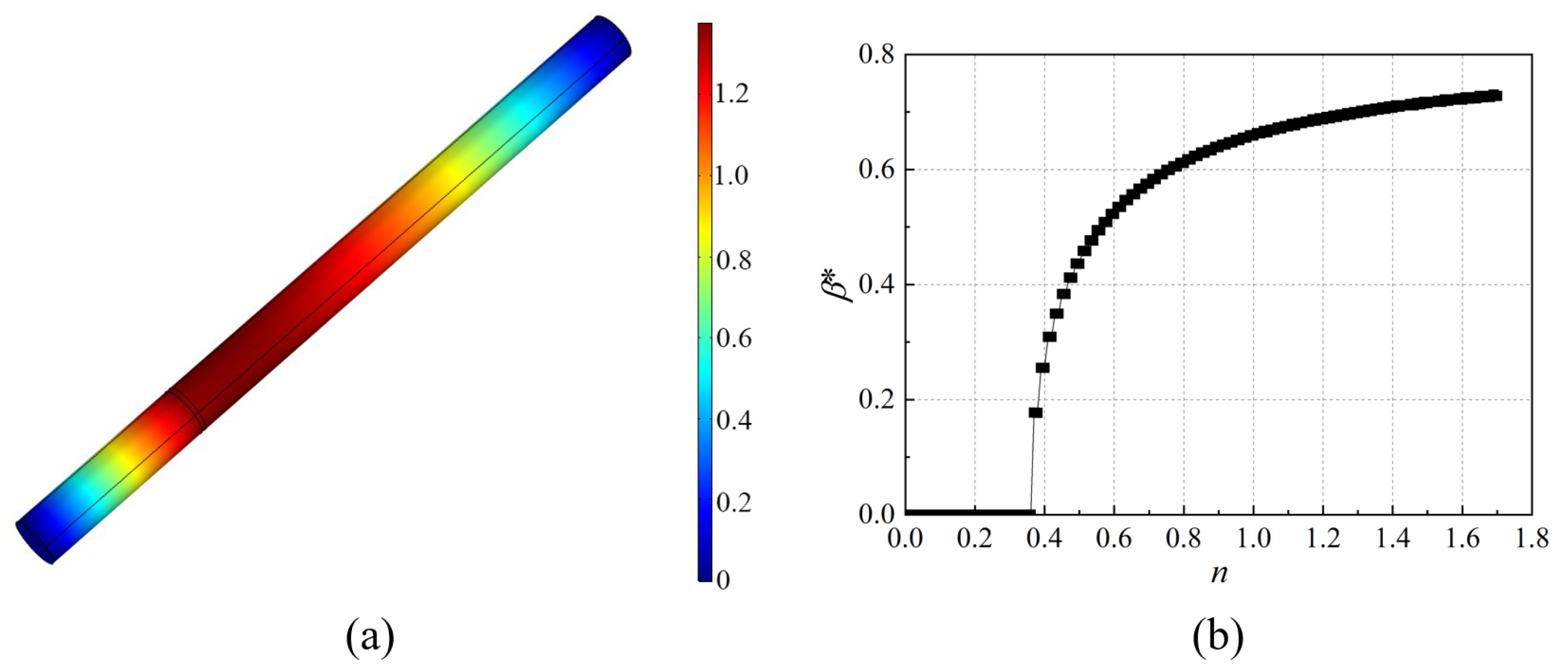
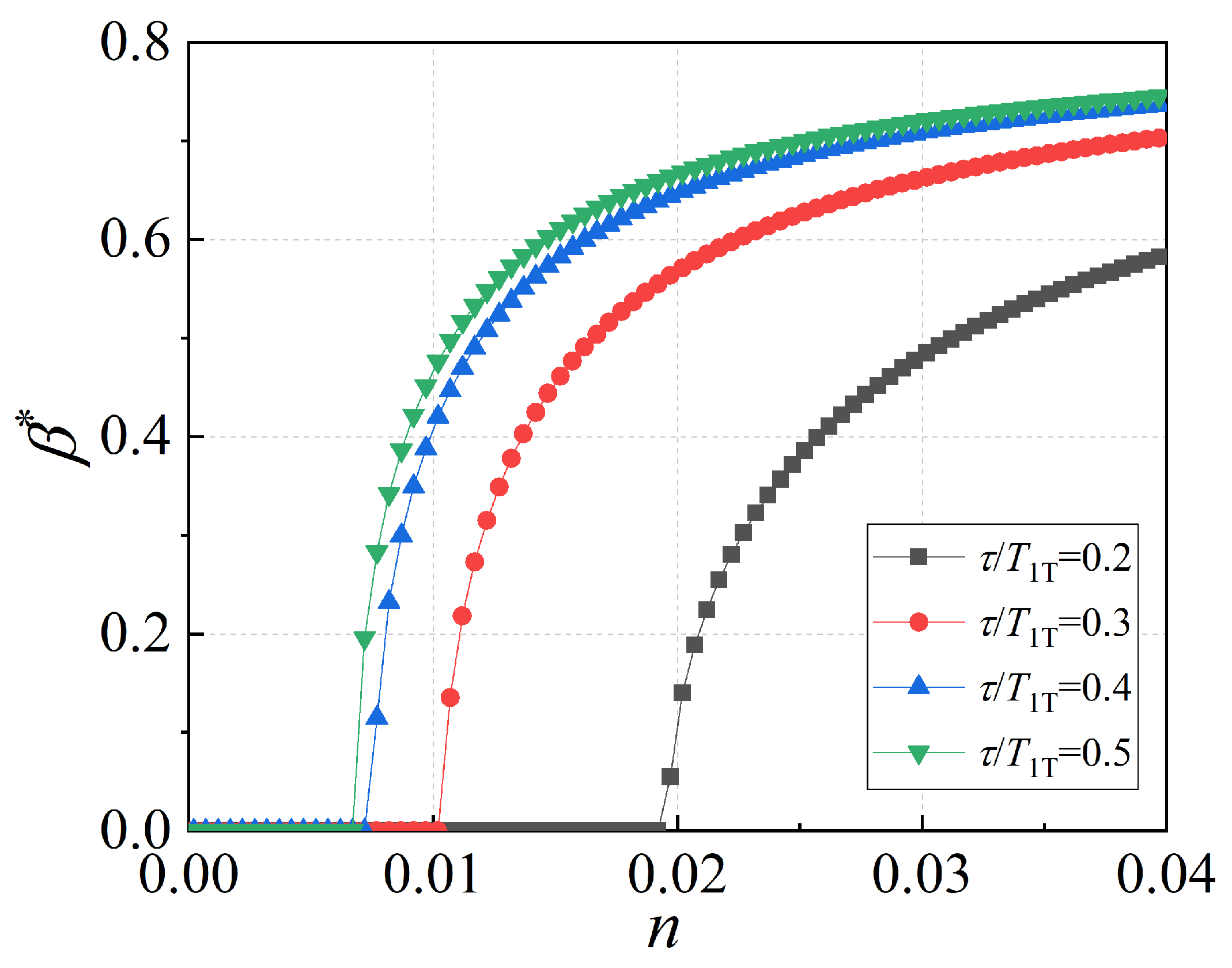
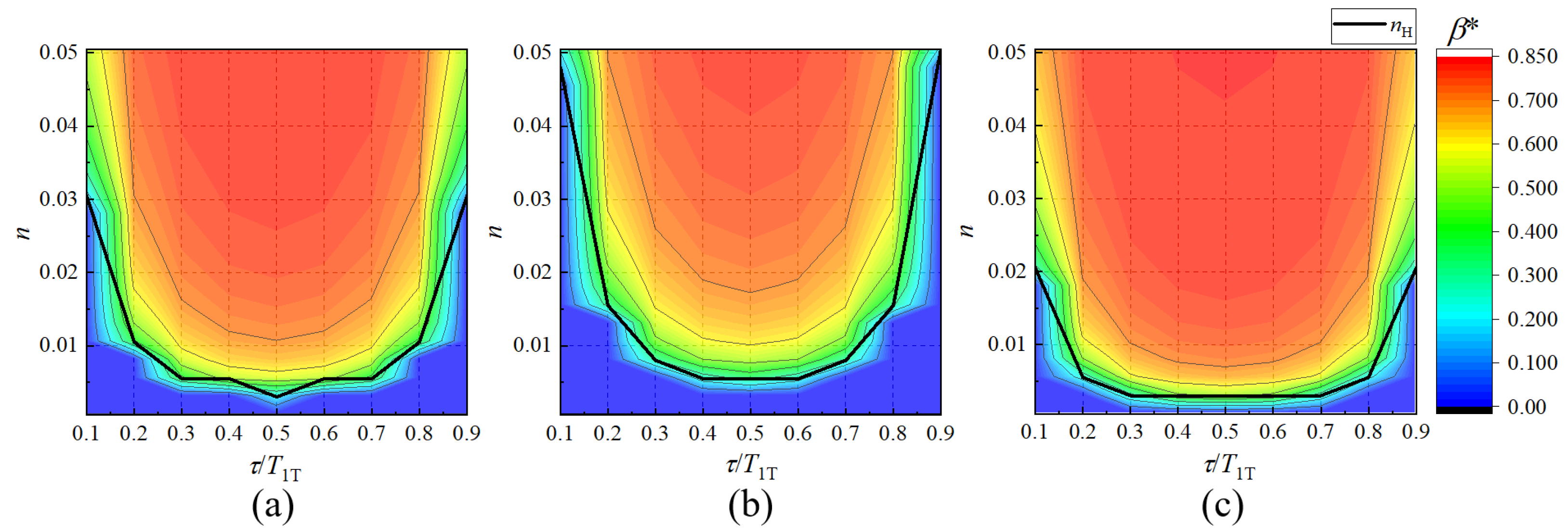
4.2. BKD Combustor with Uniform Flame 0 Distribution along the Radius

Due to the more complicated geometries and flow field in the BKD combustor, the FEM calculation becomes more complex. The grid number used for the FEM calculation is 112,008. The grid in the injection system is dense due to the small radius, while that in the combustion chamber remains coarse due to the sufficiently large acoustic wavelength. For this configuration, the global mean heat release rate is calculated by the RANS simulation; the local mean heat release rate is assumed to equal $\overline{Q}/V_{\mathrm{f}}$, where $V_{\mathrm{f}}$ again represents the volume of the flame. Thus the local heat release rate perturbation $\widehat{q}$ equals $\widehat{p}/{\overline{p}}_{\mathrm{cc}}\overline{Q}/V_{\mathrm{f}}F(\omega ,\beta )$. The Helmholtz equation was solved by the COMSOL Multiphysics to get the modal frequencies and growth rates, and further the mode shapes.

In this work, one firstly considers the situation that the flame length distribution along the radius is uniform. The frequencies of the first longitudinal and first transverse thermoacoustic modes equal 2919.3 Hz and 9096.2 Hz respectively, and their mode shapes can be viewed in Figure 7a,b. The frequency of the first transverse mode 9096.2 Hz is similar to that of experiment 10,260 Hz [27], the offset may be because of physical parameter error from RANS. It is noted that the pressure perturbations in the oxygen injection unit are both smaller than those in the combustion chamber for the two modes. For the first transverse mode, a maximum pressure perturbation is attained near the injection plate. Under these conditions, the combustor is more prone to combustion instabilities. For the first longitudinal mode, the combustion instability in the combustor behaves more like that in the Rijke tube. Furthermore, the transverse combustion instabilities are more prone to occur in the LRE combustor and are more harmful. One thus pays more attention to the first transverse mode.

One firstly considers the linear stabilities of the first transverse mode, i.e., only the linear part of the FDF is considered and $\mu =0$ in Equation (4). For the sake of simplicity, one defines a time period $T_1\mathrm{T}=1/\left(f_1\mathrm{T}\right)$, where $f_1\mathrm{T}=9096.2$ Hz. It is then possible to normalise the time delay of the FDF by this time period, as it is typically found that the modal frequency and growth rate change periodically and the period typically approximately equals the inverse of the modal frequency [12,53,66]. Figure 8 shows the linear results of the first transverse mode for different time delays $\tau$. For a small time delay $\tau /T_1\mathrm{T}$ = 0.1, the first transverse mode remains stable and the growth rate $\alpha <0$ when $n<0.08$. With increasing n, the growth rate $\alpha$ increases and equals 0 when $n=n_{\mathrm{H}}$. One considers $n_{\mathrm{H}}$ as the index value for the marginal stable situation. When n is further increased, this mode becomes unstable, and the nonlinear term should be considered. It is then possible to increase the time delay $\tau$, and results show that the trajectory of $n_{\mathrm{H}}$ also features a periodic motion. $n_{\mathrm{H}}$ reaches the maximum value of 6.787 when $\tau /T_1\mathrm{T}=1$ and has the minimum value of 0.005 when $\tau /T_1\mathrm{T}=0.5$. It should be noted that the mode is more stable for a larger value of $n_{\mathrm{H}}$, i.e., the first transverse mode is more stable when $\tau /T_1\mathrm{T}$ approaches 1 and more unstable when $\tau /T_1\mathrm{T}$ approaches 0.5. It is also interesting to note that, when $\tau /T_1\mathrm{T}\approx 1$, a small change of the time delay may lead to a large change of $n_H$, indicating that the stability of the first transverse mode is more sensitive to $\tau$ when $\tau /T_1\mathrm{T}\approx 1$ and is more inert when $\tau$ when $\tau /T_1\mathrm{T}\approx 0.5$. It is also possible to examine the change rate of the growth rate $\alpha$ with n when $n=n_{\mathrm{H}}$. The trajectory of this value $\mathrm{d}\alpha /\mathrm{d}n$ with $\tau$ is also shown in Figure 8. When $\tau /T_1\mathrm{T}\approx 0.5$, the value of $\mathrm{d}\alpha /\mathrm{d}n$ reaches the maximum value of 85 s⁻¹, indicting that the stability is more sensitive to n. When $\tau /T_1\mathrm{T}\approx 1$, $\mathrm{d}\alpha /\mathrm{d}n$ has the minimum value, and the modal stability is less sensitive to n.

One now considers the nonlinear behaviours of the first transverse mode by accounting for the full expression of the FDF (Equation (4)). Figure 9 shows the bifurcation diagrams of the first transverse mode of the BKD combustor for different time delays $\tau$. One firstly takes the diagram when $\tau /T_1\mathrm{T}=0.2$ to illustrate the bifurcation. When n is smaller than the value of Hopf point $n_{\mathrm{H}}$, the mode is stable. With increasing the value of n, the mode becomes more unstable. When n exceeds $n_{\mathrm{H}}$, the mode becomes unstable, and a limit cycle is established when $\beta ={\beta }^{*}$, where the growth rate again equals 0 and a limit cycle is established. It is noted that the value ${\beta }^{*}$ arises with increasing n. Similar to that for the Rijke tube, a supercritical bifurcation also presents. When $\tau$ changes, the change in the shape of the bifurcation diagram remains small while the location changes. Since the calculation is quasi-symmetric with the symmetric axis $\tau /T_1\mathrm{T}=0.5$, a period motion of the entire diagram with $\tau$ is also observed, which agrees with the linear analysis. It is further noted that, when $\tau /T_1\mathrm{T}$ is close to 0 or 1, the Hopf point $n_{\mathrm{H}}$ is larger and the value of ${\beta }^{*}$ is smaller. When $\tau /T_1\mathrm{T}$ is close to 0.5, the Hopf point $n_{\mathrm{H}}$ is smaller and the ${\beta }^{*}$ increases more rapidly when n is close to $n_{\mathrm{H}}$, which agrees with the results for $\mathrm{d}\alpha /\mathrm{d}n$ in Figure 8.

It is also interesting to note that the 3D diagram shown in Figure 9 degenerates to the linear stability results shown in Figure 8 when $\beta =0$. It is obvious that linear analysis is helpful even in the nonlinear studies. When using the nonlinear flame model, all disturbances finally grow or decay to zero or the values corresponding to the limit cycle state. When the nonlinear flame model is close to real dynamics flames, if possible, and the resolution of the data is high enough, the state that an arbitrary disturbance will finally reach could be predicted precisely. It is also possible to examine the relation between $\tau$ and ${\beta }^{*}$ or the $\tau -{\beta }^{*}$ bifurcation diagram based on the $\tau -{\beta }^{*}$ plane for a fixed n from the 3D diagram, as also shown in [67].

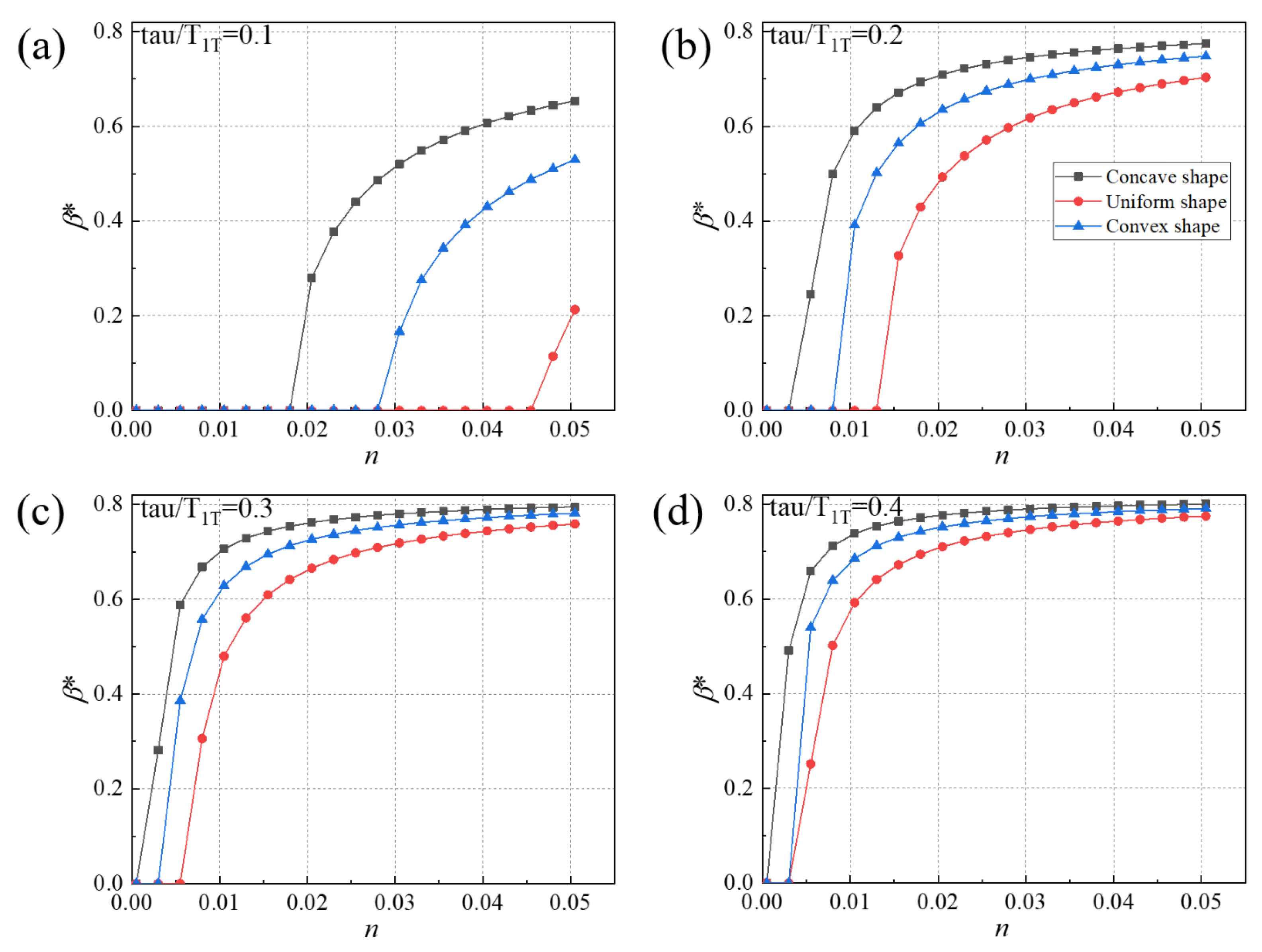
4.3. Effects of Flame 0 Distribution on the Bifurcation Diagram of the BKD Combustor

In a supercritical bifurcation system like that shown in Figure 9, there is a consistent one-to-one match between a pair of $\tau -n$ and one value of ${\beta }^{*}$; the three dimensional bifurcation diagrams of the first transverse mode for the BKD combustor thus could be shown as contour maps as shown in Figure 10. The differences among the contours for the three flame length distributions are obvious. When $\tau /T_{1\mathrm{T}}$ equals 0.5, the limit cycle for first transverse mode is established earlier for the non-uniform distributions than that for the uniform distribution. For the concave distribution, the marginal stable border is flatter, indicating that the marginal stability is more insensitive to the change of $\tau$. At the same time, the more flat concave distribution illustrates that the system would become unstable when the gain index n is low. Maybe under this situation, the heat release rate and large oscillation region of pressure disturbance are in phase well, having more volume superimposed region. Furthermore, it is noted that the first transverse mode for the BKD combustor with a non-uniform flame length distribution is more likely to attain a limit cycle with a larger perturbation amplitude.

In order to quantitatively compare the differences among results for the three flame length distributions, ${\beta }^{*}-n$ plots under different $\tau$ are extracted and shown in Figure 11. Due to the quasi-symmetric shape of the contour as a function of n (Figure 10), only results for half part are presented. Results show that the first transverse mode is more unstable for non-uniform flame length distributions. For example, when $\tau /T$ equals 0.1, the first transverse mode of the BKD combustor with concave and convex shapes enter the limit cycle when $\beta$ equals 0.018 and 0.028, and the value of ${\beta }^{*}$ is 0.0455 for the uniform distribution. Furthermore, the limit cycle value ${\beta }^{*}$ increases with increasing $\tau$ and attains the maximum value when $\tau /T_1\mathrm{T}$ is close to 0.5. This also agrees with the periodic motion as illustrated in Figure 8. Further, the concave, convex and uniform flame length distributions represent different flow rate distributions. Once the law was commanded, combustion instability could be attempted to eliminate by designing flow rate distribution. Therefore, the simulation of this paper suggested that a uniform flame shape may be a good way to control combustion instability.

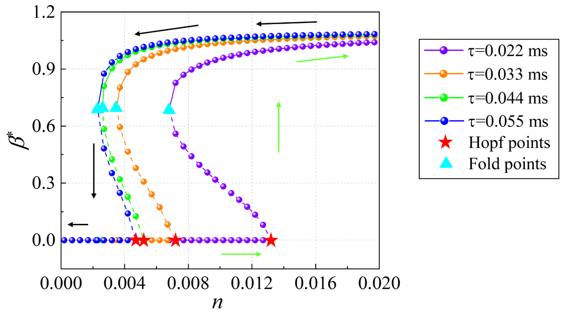
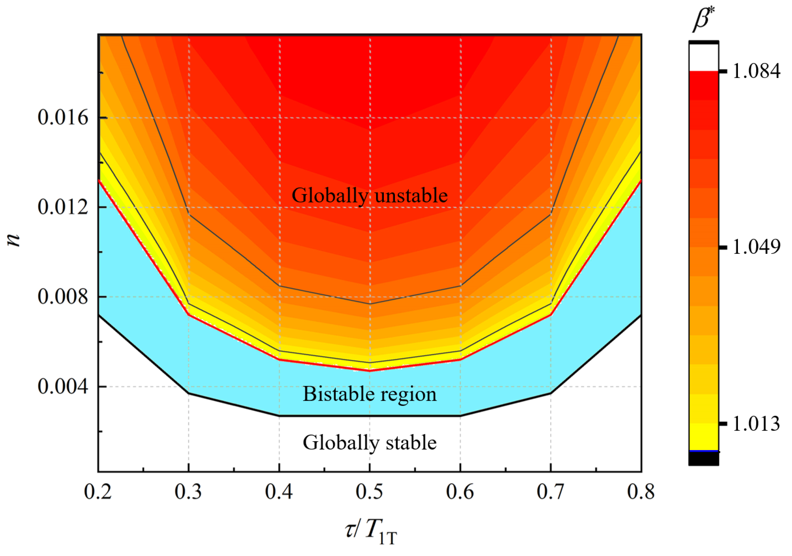
4.4. Bistable System

To investigate more complicated nonlinear behaviours of thermoacoustic instabilities, the fifth order flame describing function was accounted for in the BKD combustor with the uniform flame distribution. The phenomena of subcritical bifurcation were captured and plotted in Figure 12. Solid lines represent the stable states or limit cycles, while dashed lines indicate unstable limit cycles. Four time delays were accounted for. The green and black arrows indicate the route when the flame describing function gain index n increases and decreases, respectively. The Hopf points and the fold points were indicated by red stars and light blue triangles. Under the situation of subcritical bifurcation, these points are called subcritical Hopf bifurcation points and fold bifurcation points. When the flame describing function gain index n is between the values for the Hopf point $n_H$ and fold point $n_f$, the system is linear stable but nonlinear unstable, indicating that the system remains stable if the pressure perturbation is smaller than that for the unstable limit cycle, while the system will increase to a stable limit cycle if the pressure perturbation is larger than the value for the unstable limit cycle.

The region of stability analysis for the variation of flame describing function gain index n and the time delay $\tau$ is shown in Figure 13. The black solid line and the red solid line indicate the fold points and the Hopf points, respectively. Between them, different regions represent the different stable states. Similar to the contour of the pressure perturbation amplitude in the previous section, the lower part of Figure 13 is a globally stable region independent of the pressure perturbation amplitude. Similarly, the upper part is a globally unstable region independent of the pressure perturbation amplitude. Between them, a region that is neither globally stable nor globally unstable emerged, which considered as the bistable region. A stable steady state and a pair of stable and unstable limit cycles are included in this region. The converged state is determined by the initial pressure disturbance.

5. Conclusions

This paper analysed the nonlinear combustion instability, especially the Hopf bifurcation, of two combustors with a pressure dependent flame describing function based on the Helmholtz equation numerically resolved by the commercial software COMSOL multiphysics. The numerical method was firstly implemented on a Rijke tube combustor for validation, and a supercritical bifurcation for the first longitudinal mode was observed. The nonlinear responses and further the bifurcation diagrams of the first transverse mode for different time delay and gain index of the FDF were analysed. The change law between $n_{\mathrm{H}}$ and $\tau$ was obtained. The trajectory of Hopf points and even the bifurcation diagram feature period motions with increasing the time delay $\tau$ of the FDF. For the envisaged flame model, the supercritical bifurcation and the subcritical bifurcation can be established. The effect of flame length distributions on the bifurcation diagrams was analysed by considering a non-uniform flame length distribution model. Results showed that the first mode is more easily to attain the limit cycle and is more insensitive to the time delay for the non-uniform distribution. Furthermore, the first transverse mode for the BKD combustor with a non-uniform flame length distribution is more likely to attain a limit cycle with a larger perturbation amplitude. Finally, a subcritical bifurcation is investigated and the bistable region, linear stable but nonlinear unstable, is analysed. Due to the large scales and multiple injectors in the liquid rocket engines, the direct simulation of the combustion instabilities within these devices is much more time consuming and impossible for the engineering design. The present work decouples the flame responses simulation from the entire simulation and can be used to reduce the computing cost. Although calculation of the flame responses have not been conducted, which is replaced by a nonlinear flame response model, these results in this work is worthy for the analysis of the nonlinear behaviors of the combustion instabilities, especially for the transverse modes. The discussion on the flame response distribution may be helpful for the injector’s optimization to eliminate the combustion instability.

References

1. Eckstein, J.; Sattelmayer, T. Low-Order Modeling of Low-Frequency Combustion Instabilities in AeroEngines. J. Propul. Power 2006, 22, 425–432. [Google Scholar] [CrossRef]
2. Oefelein, J.C.; Yang, V. Comprehensive review of liquid-propellant combustion instabilities in F-1 engines. J. Propul. Power 1993, 9, 657–677. [Google Scholar] [CrossRef]
3. Pieringer, J.; Sattelmayer, T.; Fassl, F. Simulation of Combustion Instabilities in Liquid Rocket Engines with Acoustic Perturbation Equations. J. Propul. Power 2009, 25, 1020–1031. [Google Scholar] [CrossRef]
4. Lieuwen, T.C.; Yang, V. Combustion Instabilities in Gas Turbine Engines: Operational Experience, Fundamental Mechanisms, and Modeling; American Institute of Aeronautics and Astronautics: Reston, VA, USA, 2005. [Google Scholar]
5. Candel, S. Combustion dynamics and control: Progress and challenges. P Combust. Inst. 2002, 29, 1–28. [Google Scholar] [CrossRef]
6. Palies, P.; Schuller, T.; Durox, D.; Gicquel, L.; Candel, S. Acoustically perturbed turbulent premixed swirling flames. Phys. Fluids 2011, 23, 037101. [Google Scholar] [CrossRef] [Green Version]
7. Zhou, S.; Nie, W.; Tian, Y. High frequency combustion instability control by discharge plasma in a model rocket engine combustor. Acta Astronaut. 2021, 179, 391–406. [Google Scholar] [CrossRef]
8. Sujith, R.I.; Unni, V.R. Complex system approach to investigate and mitigate thermoacoustic instability in turbulent combustors. Phys. Fluids 2020, 32, 061401. [Google Scholar] [CrossRef]
9. Richecoeur, F.; Ducruix, S.; Scouflaire, P.; Candel, S. Experimental investigation of high-frequency combustion instabilities in liquid rocket engine. Acta Astronaut. 2008, 62, 18–27. [Google Scholar] [CrossRef]
10. Rijke, P.L. Notiz über eine neue Art, die in einer an beiden Enden offenen Röhre enthaltene Luft in Schwingungen zu versetzen. Ann. Der Phys. Und Chem. 1859, 183, 339–343. [Google Scholar] [CrossRef] [Green Version]
11. Dowling, A.P. The calculation of thermoacoustic oscillations. J. Sound Vib. 1995, 180, 557–581. [Google Scholar] [CrossRef]
12. Li, J.; Morgans, A.S. Time domain simulations of nonlinear thermoacoustic behaviour in a simple combustor using a wave-based approach. J. Sound Vib. 2015, 346, 345–360. [Google Scholar] [CrossRef] [Green Version]
13. Juniper, M.P.; Sujith, R. Sensitivity and Nonlinearity of Thermoacoustic Oscillations. Annu. Rev. Fluid. Mech. 2018, 50, 661–689. [Google Scholar] [CrossRef] [Green Version]
14. Dowling, A.P.; Stow, S.R. Acoustic Analysis of Gas Turbine Combustors. J. Propul. Power 2003, 19, 751–764. [Google Scholar] [CrossRef]
15. Li, J.; Yang, D.; Luzzato, C.; Morgans, A.S. OSCILOS: The Open Sounce Combustion Instability Low Order Simulator Technical Report; Technical Report; Imperial College: London, UK, 2015. [Google Scholar]
16. Balasubramanian, K.; Sujith, R.I. Thermoacoustic instability in a rijke tube: Non-normality and nonlinearity. Phys. Fluids 2008, 20, 044103. [Google Scholar] [CrossRef]
17. Etikyala, S.; Sujith, R. Change of criticality in a prototypical thermoacoustic system. Chaos Interdiscip. J. Nonlinear Sci. 2017, 27, 023106. [Google Scholar] [CrossRef] [PubMed]
18. Xi, Y.; Li, X.; Wang, Y.; Xu, B.; Wang, N.; Zhao, D. Experimental study of transition to instability in a Rijke tube with axially distributed heat source. Int. J. Heat Mass. Transf. 2022, 183, 122157. [Google Scholar] [CrossRef]
19. Li, S.; Li, Q.; Tang, L.; Yang, B.; Fu, J.; Clarke, C.; Jin, X.; Ji, C.; Zhao, H. Theoretical and experimental demonstration of minimizing self-excited thermoacoustic oscillations by applying anti-sound technique. Appl. Energ. 2016, 181, 399–407. [Google Scholar] [CrossRef]
20. Wu, G.; Lu, Z.; Pan, W.; Guan, Y.; Li, S.; Ji, C. Experimental demonstration of mitigating self-excited combustion oscillations using an electrical heater. Appl. Energ. 2019, 239, 331–342. [Google Scholar] [CrossRef]
21. Mariappan, S.; Sujith, R.I.; Schmid, P.J. Non-normality of thermoacoustic interactions: An experimental investigation. In Proceedings of the 47th AIAA/ASME/SAE/ASEE Joint Propulsion Conference and Exhibit, San Diego, CA, USA, 31 July–3 August 2011. Number AIAA-2011-5555. [Google Scholar]
22. Armbruster, W.; Hardi, J.S.; Suslov, D.; Oschwald, M. Experimental investigation of self-excited combustion instabilities with injection coupling in a cryogenic rocket combustor. Acta Astronaut. 2018, 151, 655–667. [Google Scholar] [CrossRef]
23. Armbruster, W.; Hardi, J.S.; Miene, Y.; Suslov, D.; Oschwald, M. Damping device to reduce the risk of injection-coupled combustion instabilities in liquid propellant rocket engines. Acta Astronaut. 2020, 169, 170–179. [Google Scholar] [CrossRef]
24. Hardi, J.S.; Traudt, T.; Bombardieri, C.; Börner, M.; Beinke, S.K.; Armbruster, W.; Nicolas Blanco, P.; Tonti, F.; Suslov, D.; Dally, B.; et al. Combustion dynamics in cryogenic rocket engines: Research programme at DLR Lampoldshausen. Acta Astronaut. 2018, 147, 251–258. [Google Scholar] [CrossRef]
25. Schulze, M.; Urbano, A.; Zahn, M.; Schmid, M.; Sattelmayer, T.; Oschwald, M. Thermoacoustic feedback analysis of a cylindrical combustion chamber under supercritical conditions. In Proceedings of the 50th AIAA/ASME/SAE/ASEE Joint Propulsion Conference, Cleveland, OH, USA, 28–30 July 2014; p. 3776. [Google Scholar]
26. Gröning, S.; Suslov, D.; Hardi, J.; Oschwald, M. Influence of hydrogen temperature on the acoustics of a rocket engine combustion chamber operated with LOX/H2 at representative conditions. In Proceedings of the Space Propulsion, Cologne, Germany, 19–22 May 2014. [Google Scholar]
27. Urbano, A.; Selle, L.; Staffelbach, G.; Cuenot, B.; Schmitt, T.; Ducruix, S.; Candel, S. Exploration of combustion instability triggering using Large Eddy Simulation of a multiple injector liquid rocket engine. Combust. Flame 2016, 169, 129–140. [Google Scholar] [CrossRef] [Green Version]
28. Urbano, A.; Douasbin, Q.; Selle, L.; Staffelbach, G.; Cuenot, B.; Schmitt, T.; Ducruix, S.; Candel, S. Study of flame response to transverse acoustic modes from the LES of a 42-injector rocket engine. P Combust. Inst. 2017, 36, 2633–2639. [Google Scholar] [CrossRef] [Green Version]
29. Waxenegger-Wilfing, G.; Sengupta, U.; Martin, J.; Armbruster, W.; Oschwald, M. Early detection of thermoacoustic instabilities in a cryogenic rocket thrust chamber using combustion noise features and machine learning. Chaos 2021, 31, 063128. [Google Scholar] [CrossRef] [PubMed]
30. Crocco, L. Aspects of Combustion Stability in Liquid Propellant Rocket Motors Part I: Fundamentals. Low Frequency Instability With Monopropellants. J. Am. Rocket Soc. 1951, 21, 163–178. [Google Scholar] [CrossRef]
31. Dowling, A.P. Nonlinear self-excited oscillations of a ducted flame. J. Fluid Mech. 1997, 346, 271–290. [Google Scholar] [CrossRef]
32. Schuermans, B.; Guethe, F.; Pennell, D.; Guyot, D.; Paschereit, C.O. Thermoacoustic Modeling of a Gas Turbine Using Transfer Functions Measured Under Full Engine Pressure. J. Eng. Gas Turbines Power 2010, 132, 111503. [Google Scholar] [CrossRef]
33. Schuller, T.; Poinsot, T.; Candel, S. Dynamics and control of premixed combustion systems based on flame transfer and describing functions. J. Fluid Mech. 2020, 894, P1. [Google Scholar] [CrossRef]
34. Lieuwen, T.C. Experimental investigation of limit-cycle oscillations in an unstable gas turbine combustor. J. Propul. Power 2002, 18, 61–67. [Google Scholar] [CrossRef]
35. Sun, Y.; Rao, Z.; Zhao, D.; Wang, B.; Sun, D.; Sun, X. Characterizing nonlinear dynamic features of self-sustained thermoacoustic oscillations in a premixed swirling combustor. Appl. Energ. 2020, 264, 114698. [Google Scholar] [CrossRef]
36. Flandro, G.A.; Fischbach, S.R.; Majdalani, J. Nonlinear rocket motor stability prediction: Limit amplitude, triggering, and mean pressure shift. Phys. Fluids 2007, 19, 094101. [Google Scholar] [CrossRef] [Green Version]
37. Moeck, J.; Bothien, M.; Schimek, S.; Lacarelle, A.; Paschereit, C. Subcritical thermoacoustic instabilities in a premixed combustor. In Proceedings of the 14th AIAA/CEAS Aeroacoustics Conference (29th AIAA Aeroacoustics Conference), Vancouver, BC, Canada, 5–7 May 2008; American Institute of Aeronautics and Astronautics: Reston, VA, USA, 2008. [Google Scholar]
38. Mariappan, S.; Sujith, R.I. Modelling nonlinear thermoacoustic instability in an electrically heated Rijke tube. J. Fluid Mech. 2011, 680, 511–533. [Google Scholar] [CrossRef]
39. Wang, Z.; Liu, P.; Jin, B.; Ao, W. Nonlinear characteristics of the triggering combustion instabilities in solid rocket motors. Acta Astronaut. 2020, 176, 371–382. [Google Scholar] [CrossRef]
40. Dowling, A.P. A kinematic model of a ducted flame. J. Fluid Mech. 1999, 394, 51–72. [Google Scholar] [CrossRef]
41. Schuller, T.; Durox, D.; Candel, S. A unified model for the prediction of laminar flame transfer functions: Comparisons between conical and V-flame dynamics. Combust. Flame 2003, 134, 21–34. [Google Scholar] [CrossRef]
42. Polifke, W. Modeling and analysis of premixed flame dynamics by means of distributed time delays. Prog. Energ. Combust. 2020, 79, 100845. [Google Scholar] [CrossRef]
43. Li, J.; Liu, T.; Yang, L. An analytical model for the transversely forced flame transfer functions of conical and V-flame dynamics. Fuel 2020, 276, 117987. [Google Scholar] [CrossRef]
44. Jiang, X.; Yang, L.; Liu, T.; Li, J. Nonlinear Models of Laminar Premixed Slit Flame Responses Subjected to Two-Way Perturbations. AIAA J. 2022, 60, 962–975. [Google Scholar] [CrossRef]
45. Gopalakrishnan, E.A.; Sujith, R.I. Effect of external noise on the hysteresis characteristics of a thermoacoustic system. J. Fluid Mech. 2015, 776, 334–353. [Google Scholar] [CrossRef]
46. Kabiraj, L.; Sujith, R.I.; Wahi, P. Bifurcations of self-excited ducted laminar premixed flames. J. Eng. Gas. Turb. Power 2012, 134, 031502. [Google Scholar] [CrossRef]
47. Stow, S.R.; Dowling, A.P. A Time-Domain Network Model for Nonlinear Thermoacoustic Oscillations. J. Eng. Gas. Turb. Power 2009, 131, 031502. [Google Scholar] [CrossRef]
48. Sayadi, T.; Le Chenadec, V.; Schmid, P.; Richecœur, F.; Massot, M. Time-domain analysis of thermo-acoustic instabilities in a ducted flame. P Combust. Inst. 2015, 35, 1079–1086. [Google Scholar] [CrossRef]
49. Noiray, N.; Bothien, M.; Schuermans, B. Investigation of azimuthal staging concepts in annular gas turbines. Combust. Theor. Model 2011, 15, 585–606. [Google Scholar] [CrossRef]
50. Yang, L.; Pang, B.; Li, J. Comparison of strongly and weakly nonlinear flame models applied to thermoacoustic instability. Phys. Fluids 2021, 33, 094108. [Google Scholar] [CrossRef]
51. Campa, G.; Juniper, M.P. Obtaining bifurcation diagrams with a thermoacoustic network model. In Proceedings of the Volume 2: Combustion, Fuels and Emissions, Parts A and B; American Society of Mechanical Engineers: New York, NY, USA, 2012. [Google Scholar]
52. Campa, G.; Cinquepalmi, M.; Camporeale, S.M. Influence of nonlinear flame models on sustained thermoacoustic oscillations in gas turbine combustion chambers. In Proceedings of the Volume 1A: Combustion, Fuels and Emissions; American Society of Mechanical Engineers: New York, NY, USA, 2013. [Google Scholar]
53. Laera, D.; Campa, G.; Camporeale, S. A finite element method for a weakly nonlinear dynamic analysis and bifurcation tracking of thermo-acoustic instability in longitudinal and annular combustors. Appl. Energ. 2017, 187, 216–227. [Google Scholar] [CrossRef]
54. Nicoud, F.; Benoit, L.; Sensiau, C.; Poinsot, T. Acoustic Modes in Combustors with Complex Impedances and Multidimensional Active Flames; American Institute of Aeronautics and Astronautics (AIAA): Reston, VA, USA, 2007. [Google Scholar]
55. Lin, S.C.; Bomberg, S.; Polifke, W. Propagation and Generation of Acoustic and Entropy Waves Across a Moving Flame Front. Combust. Flame 2016, 166, 170–180. [Google Scholar]
56. Lehoucq, R.B.; Sorensen, D.C.; Yang, C. ARPACK Users’ Guide; Society for Industrial and Applied Mathematics: Philadelphia, PA, USA, 1998. [Google Scholar]
57. Anderson, W.E.; Yang, V. Liquid Rocket Engine Combustion Instability—Combustion Instability Analysis: Analytical Models for Combustion Instability; The American Institute of Aeronautics and Astronautics: Reston, VA, USA, 1995; pp. 403–430. [Google Scholar] [CrossRef]
58. Noiray, N.; Durox, D.; Schuller, T.; Candel, S. A unified framework for nonlinear combustion instability analysis based on the flame describing function. J. Fluid Mech. 2008, 615, 139–167. [Google Scholar] [CrossRef]
59. Gröning, S.; Hardi, J.S.; Suslov, D.; Oschwald, M. Injector-driven combustion instabilities in a hydrogen/oxygen rocket combustor. J. Propul. Power 2016, 32, 560–573. [Google Scholar] [CrossRef]
60. Schulze, M.; Sattelmayer, T. Linear stability assessment of a cryogenic rocket engine. Int. J. Spray Combust. 2017, 9, 277–298. [Google Scholar] [CrossRef] [Green Version]
61. Duran, I.; Moreau, S. Solution of the quasi-one-dimensional linearized Euler equations using flow invariants and the Magnus expansion. J. Fluid Mech. 2013, 723, 190–231. [Google Scholar] [CrossRef]
62. Duran, I.; Morgans, A.S. On the reflection and transmission of circumferential waves through nozzles. J. Fluid Mech. 2015, 773, 137–153. [Google Scholar] [CrossRef] [Green Version]
63. Duchaine, F.; Boudy, F.; Durox, D.; Poinsot, T. Sensitivity analysis of transfer functions of laminar flames. Combust. Flame 2011, 158, 2384–2394. [Google Scholar] [CrossRef]
64. Hwang, W.S.; Sung, B.K.; Han, W.; Huh, K.Y.; Lee, B.J.; Han, H.S.; Sohn, C.H.; Choi, J.Y. Real-Gas-Flamelet-Model-Based Numerical Simulation and Combustion Instability Analysis of a GH2/LOX Rocket Combustor with Multiple Injectors. Energies 2021, 14, 419. [Google Scholar] [CrossRef]
65. Armbruster, W.; Hardi, J.S.; Oschwald, M. Flame-acoustic response measurements in a high-pressure, 42-injector, cryogenic rocket thrust chamber. P Combust. Inst. 2021, 38, 5963–5970. [Google Scholar] [CrossRef]
66. Silva, C.F.; Nicoud, F.; Schuller, T.; Durox, D.; Candel, S. Combining a Helmholtz solver with the flame describing function to assess combustion instability in a premixed swirled combustor. Combust. Flame 2013, 160, 1743–1754. [Google Scholar] [CrossRef] [Green Version]
67. Subramanian, P.; Mariappan, S.; Sujith, R.I.; Wahi, P. Bifurcation analysis of thermoacoustic instability in a horizontal rijke tube. Int. J. Spray Combust. 2010, 2, 325–355. [Google Scholar] [CrossRef]
Figure 1. Model and mesh of Rijke tube.
Aerospace 09 00593 g001
Figure 2. FEM model of BKD combustor. The flame region is assmued and represented by the red block.
Aerospace 09 00593 g002
Figure 3. The acoustic reflection coefficient of the nozzle determined by the Magnus expansion of the linearised Euler equations of the nozzle.
Aerospace 09 00593 g003
Figure 4. Mean flow properties along the axis of the BKD combustion chamber obtained by the RANS simulation.
Aerospace 09 00593 g004
Figure 5. Flame lengths as a function of the radius r for the three kinds of distribution shapes.
Aerospace 09 00593 g005
Figure 6. (a) First order longitudinal mode of pressure perturbation in the Rijke tube; (b) Bifurcation diagram of the Rijke tube describing oscillation condition ( β * ) for different index n of the flame describing function.
Aerospace 09 00593 g006
Figure 7. Pressure mode-shapes of (a) the first longitudal and (b) the first transverse thermoacoustic mode. The contour map of the cross-sectional surface is at 0.015 m. Herein, n = 0 .
Aerospace 09 00593 g007
Figure 8. Evolutions of the value of n H when the thermoacoustic mode is marginal stable (corresponding to the left vertical axis) and d α / d n (corresponding to the right vertical axis) with the normalised time delay τ / T 1 T for the linear stability of the first transverse mode.
Aerospace 09 00593 g008
Figure 9. Bifurcation diagrams of the first transverse mode of the BKD combustor for different time delay τ of the FDF.
Aerospace 09 00593 g009
Figure 10. Contour of the pressure perturbation amplitude β * for the limit cycle as functions of n and τ / T 1 T for three flame length distributions: (a) convex distribution, (b) uniform distribution and (c) concave distribution. The thick lines correspond to marginal stable boarders or the lines of Hopf points.
Aerospace 09 00593 g010
Figure 11. The bifurcation diagrams for three flame distribution shapes and different time delay τ . (a) τ / T 1 T = 0.1 ; (b) τ / T 1 T = 0.2 ; (c) τ / T 1 T = 0.3 ; (d) τ / T 1 T = 0.4 .
Aerospace 09 00593 g011
Figure 12. The bifurcation diagrams for the fifth order FDF. The green arrows represent the system developing direction when the gain n increases, the black arrows represent the system developing direction when the gain n decreases.
Aerospace 09 00593 g012
Figure 13. The region of bistablility.
Aerospace 09 00593 g013