Abstract
The transport characteristics of the unsteady flow field in rarefied plasma plumes is crucial for a pulsed vacuum arc in which the particle distribution varies from 1016 to 1022 m−3. The direct simulation Monte Carlo (DSMC) method and particle-in-cell (PIC) method are generally combined to study this kind of flow field. The DSMC method simulates the motion of neutral particles, while the PIC method simulates the motion of charged ions. A hybrid DSMC/PIC algorithm is investigated here to determine the unsteady axisymmetric flow characteristics of vacuum arc plasma plume expansion. Numerical simulations are found to be consistent with the experiments performed in the plasma mass and energy analyzer (EQP). The electric field is solved by Poisson’s equation, which is usually computationally expensive. The compressed sparse row (CSR) format is used to store the huge diluted matrix and PETSc library to solve Poisson’s equation through parallel calculations. Double weight factors and two timesteps under two grid sets are investigated using the hybrid DSMC/PIC algorithm. The fine PIC grid is nested in the coarse DSMC grid. Therefore, METIS is used to divide the much smaller coarse DSMC grid when dynamic load imbalances arise. Two parameters are employed to evaluate and distribute the computational load of each process. Due to the self-adaption of the dynamic-load-balancing parameters, millions of grids and more than 150 million particles are employed to predict the transport characteristics of the rarefied plasma plume. Atomic Ti and Ti2+ are injected into the small cylinders. The comparative analysis shows that the diffusion rate of Ti2+ is faster than that of atomic Ti under the electric field, especially in the z-direction. The fully diffuse reflection wall model is adopted, showing that neutral particles accumulate on the wall, while charged ions do not—due to their self-consistent electric field. The maximum acceleration ratio is about 17.94.
1. Introduction
Plasma plumes are widely used in plasma thrusters [1], micro-cathode vacuum arc thrusters [2], space thrusters [3], industrial coatings [4], and nuclear reactors [5]. In these devices, where plasma arc jets flow, the dimensions can be relatively small, resulting in a non-continuous flow field. As the resulting plasma jet is rarefied, it is often called a plasma plume. In plasma plumes induced by pulsed vacuum arcs, the coupling characteristics of the flow field and electric field are significant. There are several components in plasma plumes, including neutral particles, charged ions, metal atoms, and electrons. These particles collide with one another to cause energy exchanges or chemical reactions. Ion motion is more complex under the action of an external electric field. There are many physical processes and different physical models in plasma plumes. Thus, it is important to study the temporal and spatial distributions and the evolutionary characteristics of plasma plumes to upgrade plasma devices.
The direct simulation Monte Carlo (DSMC) method and particle-in-cell (PIC) method are generally combined to study plasma plumes. The DSMC method is employed primarily to simulate the physical behaviors of neutral particles, while the PIC method is employed to simulate the physical behaviors of charged ions. The DSMC method is a numerical Monte Carlo approach developed by Bird [6] that directly simulates physical processes; he later showed its consistency with Boltzmann’s equation [7]. The DSMC does not solve Boltzmann’s equation to calculate the macroscopic flow field quantity, but it arranges many simulation molecules in the flow field. Each simulation molecule represents many real particles to simulate the physical processes described by the equation. Pham-Van-Diep et al. [8] used the DSMC method to study hypersonic shock wave structures in 1989. The results established the position of the DSMC method in rarefied gas dynamics, and have since been widely investigated in engineering practice. With improvements to the DSMC method and the enrichment of physical models, the DSMC method has gradually been used to solve problems in thermochemical non-equilibrium [9], thermal radiation [10], gas–solid interactions [11], and laser transmission [12].
The PIC method is a plasma particle simulation method developed by Buneman [13] and Eldridge and Feix [14] around 1960. After the PIC method was proposed, Buneman and Hockney et al. [15] solved Poisson’s equation discretely using the spatial difference method around 1965 after the development of the point superparticle [16] and the finite-size particle [17]. Since then, the PIC method has been widely used to numerically simulate electric propulsion plasma plumes and other fields. After years of development, the PIC method has been successfully applied to plasmas and can be used to solve a variety of complex physical problems [18].
In view of the remarkable multifield coupling characteristics, the hybrid DSMC/PIC algorithm is proposed to study the temporal and spatial distribution characteristics of vacuum arc plasma plumes. The particle distribution of vacuum arc plasma plumes varies from 1016 to 1022 m−3, spanning multiple orders of magnitude. Thus, tens of millions of grids and hundreds of millions of particles are required for effective simulations, which benefit from large-scale parallel computing [19]. There has been significant research on plasma plumes using parallelized DSMC or PIC methods [20], which have provided meaningful research results. In 2015, Zhang [21] performed measurement experiments on steady-state plasma thrusters. A three-dimensional hybrid DSMC/PIC model was constructed, and CUDA parallel technology was used. In 2016, Copplestone et al. [22] designed and studied a parallel algorithm for a hybrid DSMC/PIC program using the MPI message-passing model and simulated the diffusion process of plasma plumes. On a three-dimensional unstructured grid, the electric field was solved based on an HPC system, and the parallel design of the PIC was completed. In 2016, Shmelevet al. [23] simulated the expansion of a vacuum arc plasma plume in the spark stage based on a DSMC/PIC method and a dual-fluid MHD (magnetohydrodynamics) model. In 2018, Jambunathan and Levin [24] proposed a coupled calculation framework for multi-GPU simulations of particles and electrons in plasma plumes. In 2022, Gwanyong Jung and Hong-Gye Sung [25] analyzed the performance parameters of Hall thruster plumes and their abnormal electron transport based on a two-dimensional axisymmetric DSMC/PIC method.
2. The Hybrid DSMC/PIC Algorithm and Its Parallelization
Several components make up plasma plumes. Neutral particles generally move slowly, ions move slightly faster under the action of electric fields, and electrons move more quickly due to their relatively small mass. Therefore, there are three associated timesteps in the numerical simulations. There is a significant difference between the electron timestep and those for the neutral particles and charged ions. When electrons are simulated as particles, the number of calculations increases sharply. In the vacuum arc expansion stage, the main stream adopts the quasi-neutral hypothesis, ignores the influences of the sheath and secondary electron emission, and numerically simulates neutral particles and charged ions [26].
The DSMC program is written in Fortran, the PIC program is written in C++, and the hybrid DSMC/PIC algorithm is realized by hybrid Fortran and C++ programming. The PIC module is added based on the DSMC module, which is used to simulate all physical processes related to neutral particles, including collisions between neutral particles, collisions between neutral particles and charged ions, chemical reactions involving neutral particles, and wall chemical reactions. The PIC tracks the accelerated motion of charged ions under the action of an electric field and deals with the interactions between charged ions and the wall.
In the vacuum arc plasma plume’s expansion process, the electric field can be obtained by solving the electrostatic Poisson equation. Maxwell’s equation can be written under the condition of an electrostatic field as follows:
Under this approximation, the electric field can be expressed as the negative gradient of the scalar potential, which gives Poisson’s equation as follows:
Assuming that the electrons obey the Boltzmann equilibrium distribution [27], the expression for the nodal charge density is as follows:
where is the node potential, Te is the electron temperature, is the electron number density, and is the ion number density. It is assumed that positively charged ions contain only one positive charge. Under the quasi-neutrality assumption, . When or , the expression of the electric field intensity can be obtained as follows:
The hybrid algorithm uses the finite volume method for interpolation. The charged particles traverse the grid to where the node belongs. The charged particles and polyhedron with the center point of each edge of the grid are then taken as the vertex. The proportion of the corresponding grid volume is occupied, and the node charge is interpolated to obtain the grid node charge density . This can be substituted into a discrete relationship based on the grid topology relationship K = b. The potential and electric field intensity E are then computed. The serial program employs the LU decomposition method to solve for the stiffness matrix K. The flowchart for the hybrid DSMC/PIC algorithm is given in Figure 1, based on the individual flowcharts of the base programs. The implementation steps of the hybrid algorithm are introduced with the flowchart.

Figure 1.
Flowchart of the hybrid DSMC/PIC algorithm.
We used Bird’s phenomenological chemical reaction model [28]. For example, for the simulations including H2, H, X (metal atom), H2+, and H+, the hybrid code considers the following dissociation and combination chemical reactions:
where Y represents any particles in the flow field. The combination reaction in the code employs Bird’s chemical reaction model [29]. The dissociation reaction adopts the coupling model of diatomic molecular vibrational excitation and dissociation reactions [29]. More details can be found in [29]. We also consider the CEX collisions.
H2 + Y → H + H
H + H + Y → H2 + Y
H+ + H→ H + H+
H2+ + H → H2 + H+
2.1. Implementation Method of the Hybrid DSMC/PIC Algorithm
2.1.1. Reading Grid Data
The program uses a tetrahedral unstructured mesh. The mesh data contain not only the information for each mesh, but also the information for adjacent meshes. The commercial software Salome is used to generate and divide the data into two grid sets, and then the grid-processing program is used to read the grid data, calculate the parameters (such as the grid center), determine the volume and area, find the adjacent grid for each grid and the number of grids contained in each node, determine the grid surface on all boundaries, and calculate the internal normal direction of each edge interface. The grid information is processed, and the information required by the DSMC and PIC is stored in a file. The grid information required by the DSMC is different from that required by the PIC. The DSMC grid is the basic unit to handle collisions, sorting, and macro-quantity statistics between all simulated molecules. This deals with the chemical reactions of neutral particles, gas–wall interactions, and other modules separately. This helps address the movement of charged ions, the gas–wall interaction module, solutions of potential and electric fields, and the potential outputs based on nodes from the PIC grid.
2.1.2. Initialization
Initialization includes the DSMC, PIC, and the hybrid program. The initialization of the DSMC is primarily to read the grid data, dynamically store the array size with various pieces of information based on the grid data, provide the injected particle information, select the weight factor and timestep, and calculate the information for collision pairs based on the type of injected particle. If the flow field is not in a vacuum at the initial time, the background simulation molecules need to be arranged during the initialization. The PIC initialization is primarily to read the grid data, open the array of stored data in the pointer form based on the grid data, construct the stiffness matrix K to solve Poisson’s equation, and give the initial potential boundary conditions. The initialization of the hybrid program establishes the topological relationship between the two grid sets, mainly considering the conversion between neutral particles and charged ions to facilitate the interactions of particle information. For example, when executing the motion module for charged particles under an electric field in the PIC, neutral molecules are generated if they touch the wall. It is necessary to find the DSMC grid number of neutral particles from the PIC grid number of ions.
2.1.3. Particle Injection
Particle injection can be divided into neutral particles and charged ions. As the densities of neutral particles and charged ions differ by more than one or two orders of magnitude, their timesteps and weight factors are different. Thus, the neutral particles and charged ions are injected separately but using the same injection method. These are all based on the Maxwell distribution at a given velocity. The incoming particles have a unique number that ranks all charged ions and neutral particles.
2.1.4. Particle Motion
The particles begin to move after the simulated molecular injection. Particle motion is divided into two parts: The first part is the motion of neutral particles, which is processed based on the traditional DSMC processing. These particles move in uniform straight lines within a given timestep. This step includes handling the role of neutral particles and boundaries, such as the wall reflection and chemical reaction models. The particle information is passed to the PIC module through the array. The second part is the motion of charged ions. Some charged ions accelerate under the action of the electric field, which includes the wall reflection and wall chemical reaction models. Poisson’s equation is solved based on the ion information after the movements to calculate the electric field. As the charged ions move in one timestep under the action of the electric field, collisions and wall interactions between charged ions occur. After the movement of charged ions is completed, the information on their velocity and position is assigned to the queue array. After reading the data and obtaining the current particle information, the DSMC module readjusts the global number of simulation molecules based on the increase or decrease in the numbers of charged ions and neutral particles to ensure the uniqueness and correctness of the global number for the simulation molecules.
After particle movement, the hybrid DSMC/PIC algorithm adopts the same method as the general DSMC, which is to reorder the particles, select collision pairs, handle the collision and energy distributions between particles, deal with the chemical reactions of the labeled molecules involved in the chemical reactions, and calculate the velocity and direction of the species involved in the chemical reactions. The time information is stored in a file to read the data and calculate the macro-quantities during post-processing. If the simulation time is not reached, additional particles are injected. If the simulation time is reached, the cycle is stopped.
2.2. Parallel Strategy of the Hybrid DSMC/PIC Algorithm Based on MPI
As the array size of the Fortran programming language is fixed, C++ is used, as the array can be automatically expanded to meet the requirements of the continuous injection of simulation molecules into the entry surface for large-scale calculations. The pulsed vacuum arc plasma has strong spatial and temporal heterogeneity. After the arc is formed (just as the particles are emitted), the particle density near the inlet is high, and there are nearly no particles in other areas. Then, the coupling effect of the flow field and electric field is relatively strong. The electric field accelerates the movement of ions, and changes in the electric field gradient caused by ion movement become more intense.
The heterogeneity of the plume’s flow field increases with time. Neutral particles are generated after charged ions interact with the wall at speeds that are two orders of magnitude different from that of the main stream, resulting in the accumulation of neutral particles on the wall. Therefore, in addition to the conventional partition for parallel computing, it is necessary to implement a dynamic partition strategy for the grid of the computational domain with time [24]. As two sets of grids are used and their topological relationship is established, zoning is performed on the coarse DSMC grid.
METIS is selected for high-quality grid partitioning. It has the advantages of fast grid division, high execution efficiency, and fewer data interactions. The grid can be divided into k grid blocks. Using the Metis_PartGraphkway diagram splits the interface, and the specific process is as follows:
- (1)
- Each mesh is regarded as the vertex of a graph.
- (2)
- The adjacent faces of the mesh are regarded as edges in the graph.
- (3)
- The adjacency relationship of each vertex in the graph is calculated.
- (4)
- The graph partition interface is used and the number of partition domains is given.
- (5)
- The subdivision results are determined, describing what process each vertex (mesh) corresponds to.
When the load is unbalanced and the grid is repartitioned, the Kuhn–Munkres algorithm is used to allocate K grid blocks between the processors. The experience of large-scale parallel numerical simulations of plasma plumes suggests that the communication process and particle positioning in the partition account for 40% of the calculation time [24]. As the plume expands and the ions accelerate, particles often move to other partitions. The traditional CFD ghost grid method is not efficient. Therefore, the communication methods of the centralized communication strategy and distributed communication strategy are compared to improve the communication efficiency. Both strategies are implemented in the DSMC_Exchange and PIC_Exchange. Thus, the performance of the two strategies may vary on different HPC platforms, which feature various computing and communication capabilities under the different simulation configurations [30].
When the unstructured PIC grid is sized at tens of millions, there are approximately two million nodes, and the stiffness matrix K of the discrete electrostatic Poisson equation has an order of magnitude corresponding to the number of grid nodes. The data are stored in the compressed sparse row (CSR) format, and the KSP solver is called from the PETSc library and solved through parallel calculations. The equilibrium parameter threshold is set based on the development of the flow field and fixed time intervals. The time to solve Poisson’s equation and the particle migration of each process is determined, and the dynamic load balance is checked by the load imbalance factor (Lif).
where the subscripts max and min indicate the maximum and minimum time, respectively, / is the total execution time, and / and / are the times for the particle migration and to solve Poisson’s equation, respectively.
When the load is unbalanced, the grid is again divided using METIS. The load of each region needs to be counted in real time, so the weight load model (wlm) is employed. The time cost for neutral particle motion and charged ions from solving Poisson’s equation is considered. The weight parameters wlmi of a region include the numbers of neutral particles and charged ions in the grid, as well as the weight and adjustment parameters, as follows:
where and represent the numbers of neutral particles and charged ions in the area, respectively, while and are their associated weights. Selecting the appropriate K value based on the grid improves the parallel efficiency.
The parallel algorithm program for the hybrid DSMC/PIC algorithm is shown in Figure 2. Compared with Figure 1, the parallel algorithm is more complicated than the serial algorithm because of the necessity of particle exchange between processes, the dynamic load balancer, etc., led by multiple processes. For more detailed parallel strategies and communication details, see [30]. Based on the selection criteria of the key parameters in the DSMC and PIC modules, the hybrid DSMC/PIC algorithm has special requirements for parameter selection. The grid scale, timestep, weight factor, and load balancing parameters should meet the requirements of both the DSMC and PIC modules. The selection method for the key parameters of the hybrid DSMC/PIC algorithm is introduced in detail below.
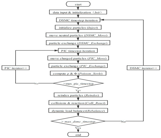
Figure 2.
DSMC/PIC flowchart for the parallel algorithm [30].
2.3. Selection of Key Parameters for the Hybrid DSMC/PIC Parallel Algorithm
2.3.1. Grid Scale
The grid scale requirement of the DSMC method is based on the molecular average free path:
where d is the average molecular diameter, and n is the number density of particles in the mesh. The PIC is based on the Debye length, which is given as follows:
where is the vacuum dielectric constant, K is Boltzmann’s constant, T is the electron temperature, n is the average ion density, and e is the electron charge.
In the plasma plume, if there is little difference between the number densities of neutral particles and charged ions, it will result in variations of several orders of magnitude between the average free path of the neutral particles and the Debye length of the charged ions [24]. In this case, two sets of grids must be used so that the grid scales meet the requirements of the DSMC and PIC modules. The fine mesh meets the requirements of the PIC Debye length, while the coarse mesh meets the requirements of the DSMC average free path.
2.3.2. Weight Factor
There is a significant difference between the number density of neutral particles and the number density of charged ions in the flow field. Thus, double weight factors must be used so that the simulated numbers of neutral particles and charged ions meet the requirements. The use of double weight factors brings difficulties in the simulations of collisions between molecules and other physical models, because the weights of simulated molecules differ, indicating that they need special treatment.
2.3.3. Timestep
Due to their grid requirements, the timesteps of neutral particles and charged ions usually differ by 1–2 orders of magnitude; therefore, two timesteps are adopted. Charged ions move multiple timesteps within a single timestep of neutral particle motion. Neutral particles are assumed to be stationary within the ionization motion timestep to ensure the unity of physical time.
2.3.4. Load Balancing Parameters
The dynamic balance weight parameters are fixed as = 1 and = 2, as seen in Equation (12). The time cost is constant as Poisson’s equation solver is fixed, which sets the parameters. The K value needs to be selected empirically based on the grid size [30].
3. Case Study of the Hybrid DSMC/PIC Algorithm
To consider the grid requirements of the DSMC and PIC modules, different neutral particles and charged ion number densities were injected to ensure that the grid scales can simultaneously met the requirements. Thus, the average free path of the neutral particles and the Debye length of the charged ions were of the same order of magnitude. The geometric model shown in Figure 3 was selected based on the calculation scale. We performed three-dimensional computation. The disk with a round hole on the left was grounded, and the disk on the right was connected with a constant bias voltage of −50 V. Considering the spatial diffusion effect of the particles, the mesh was locally densified in the small cylinder area near the injection surface. There were 292,471 coarse meshes with 51,850 mesh nodes, and there were 2,242,948 fine meshes with 383,961 mesh nodes. A large-scale performance evaluation was previously performed on the Tianhe-2 supercomputer [31]. Each Tianhe-2 node contains two Intel Xeon E5-2692 v2 processors and three Intel MIC Xeon Phi 31S1P coprocessors. Each CPU has 12 cores running at 2.2 GHz, which share a 64 GB memory.
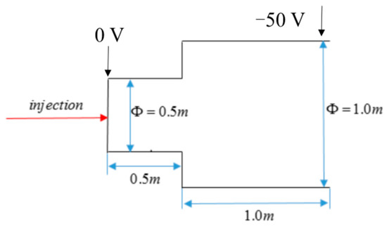
Figure 3.
Geometric model.
Atomic Ti was implanted into the coarse grid, and Ti2+ was implanted into the fine grid. The associated component parameters are shown in Table 1. A double weight factor was adopted due to the large differences between the number density of atomic Ti and that of Ti2+. The collisions between different weight factors were realized through the splitting and merging of simulated molecules. However, the number density difference between atomic Ti and Ti2+ was of 10 orders of magnitude. Thus, the associated collisions were primarily elastic. As the number density of atomic Ti was high, the VSS molecular model was adopted based on the collisions between different Ti particles, the Larsen–Borgnakke model was adopted for the collision energy distribution, and the complete diffuse reflection model was adopted for the wall, where the wall temperature was 300 K. The potential boundary was interpolated using the finite volume method, with an initial value of zero. More than 150 million particles were employed to predict the transport characteristics of the rarefied plasma plume.

Table 1.
Hybrid DSMC/PIC algorithm injection parameters.
Figure 4 shows the distributions of the atomic Ti and Ti2+ number densities at different times on the x = 0 plane. The distribution trend of the atomic Ti number density at t = 120 us flows toward the boundary, and there is no atomic Ti in the reflux area on the left of the large cylinder, indicating that atomic Ti does not completely diffuse to fill the entire space. The distribution area of the Ti2+ number density is larger than that of atomic Ti. A portion of the Ti2+ moves faster and forms a larger gradient for the self-consistent electric field. Under the action of this self-consistent electric field, a portion of the Ti2+ further accelerates. The diffusion region of Ti2+ along the axis is larger, and a wider range for the low-density region appears after the high-density region. However, there is still no Ti2+ in the reflux area on the left side of the large cylinder, indicating that it does not diffuse into the entire space and does not reach a steady flow at 160 us. Comparing the number density distributions shows that the high-density region of atomic Ti is distributed in a balloon shape, while the high-density region of Ti2+ only appears in the region near the implantation surface on the left side of the small cylinder. This indicates that the diffusion speed of Ti2+ under the action of an electric field is faster than that of atomic Ti.
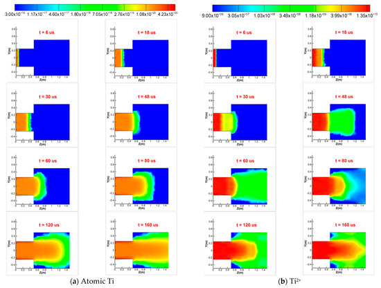
Figure 4.
Number density distributions of atomic Ti and Ti2+ at different times on the x = 0 plane.
Due to the complete diffuse reflection model adopted at the wall, the particle velocity follows a Maxwell distribution that is fully adapted to the wall temperature of 300 K. The macro flow velocity is approximately 10,000–15,000 m/s near the axis of the small cylinder—two orders of magnitude higher than the velocity reflected by the Maxwell distribution near the wall. However, we can see that neutral particles initially begin to accumulate on the wall at 30 us, while charged ions have no high-density area on the wall after the complete diffuse reflection, which is the same as for the neutral particles. When charged ions accumulate on the wall, a self-consistent electric field with a large gradient is formed locally, which accelerates the departure of ions. This is different from the formation speed of ions acting on the wall, and the effect of ion accumulation weakens. In addition, the number density difference between atomic Ti and Ti2+ is of 10 orders of magnitude. Under collision with mainstream particles, ions quickly spread out, making it difficult to form a high-density area. Neutral particles do not have this acceleration effect and rely only on collisions with the mainstream high-speed particles to weaken wall accumulation. Thus, the accumulation of neutral particles shows a doubling trend.
The accumulation of neutral particles near the wall makes the velocity along the z-axis smaller than before, because slow particles increasingly contribute to the flow. This is analogous to the small cylinder becoming thinner. Figure 5 shows that the number density of atomic Ti from the outlet of the small cylinder falls more slowly than before.
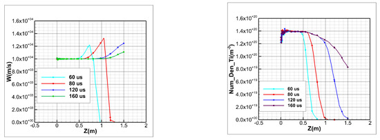
Figure 5.
Velocity and number density distribution of atomic Ti at different times on the x = 0 plane.
Figure 6 shows the potential distribution at different times on the x = 0 plane. The axial potential is the greatest near the injection surface and the least near the right-end wall. As the right-end potential is the first type of boundary condition, the potential in the nearby area is the lowest. The potential changes fastest over x = 0.5 m and x=1.4 m. Due to the quasi-neutral assumption, the potential is determined primarily by the number density of the charged ions. The ions at the outlet of the small cylinder expand to vacuum, and the gradient of the number density changes greatly over x = 0.5 m. On the other hand, the outlet at the right end is the first type of boundary condition. For elliptic equations, such as Poisson’s equation, the first type of boundary significantly impacts the calculation results. Over time, the potential near the injection surface gradually increases until reaching a stable value. Compared with ions that accelerate in the electric field and vacuum, the continuously injected ions in the flow field become slower over time. This results in aggregation near the injection surface and a gradual development toward the outlet, and gradually increases the potential near the injection surface. The high-density region of ions also gradually develops forward and reaches stability. For most of the flow, the potential is close to 0 V, and the number density is highest near the injection surface. The vacuum arc plume expands to vacuum most of the time, so the electric field gradient in the radial direction of the large cylinder is smaller than in the axial direction.
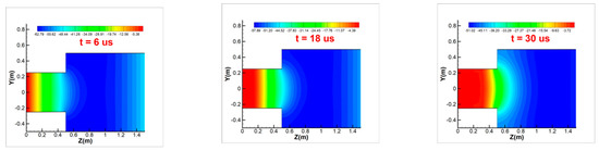
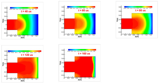
Figure 6.
Potential distribution at different times on the x = 0 plane.
Figure 7 shows the variation curve for the potential along the z-direction at different times on the axis of symmetry. The potential near the injection surface is close to zero, and the potential gradually decreases with the distance along the z-direction. After z = 0.5 m, the potential changes nearly linearly toward the outlet. The potential near the maximum of the given value of the first type of boundary is −50 V. As ions do not fill the entire space before 48 us, the potential in some vacuum areas is less than −50 V. Over time, the overall potential gradually increases, but the trend is less obvious before finally tending to be near a stable value. At greater distances along the z-direction, the difference in the potential at different times gradually decreases. As ions fill the space, they show quasi-neutral characteristics, and the potential is close to zero overall.
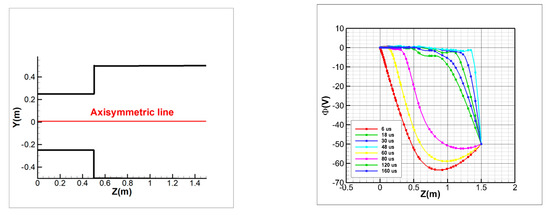
Figure 7.
Variation curves of the potential along the z-direction at different times on the axis of symmetry.
Figure 8 shows the variation curves for the number densities of atomic Ti and Ti2+ along the z-direction at different times on the symmetry axis. Before t = 30 us, atomic Ti does not move to the right-end face, and the number density rapidly decreases to zero. Over time, atomic Ti gradually diffuses along the z-direction, and the number density gradually increases. After t = 30 us, atomic Ti moves to the right-end plane, and the number density gradually increases and keeps approaching the inlet number density. From the variation curves of the Ti2+ number density, when t = 6 us, Ti2+ does not move to the right-end face, and the number density rapidly decreases to zero. At t = 48 us, Ti2+ diffuses to the right-end face but decreases rapidly along the z-direction before decreasing slowly and then decreasing rapidly. Over time, the number density of Ti2+ at the same position gradually increases to a stable value. The difference between the variation trends of the atomic Ti and Ti2+ number densities is that after the particles fill the space, the number density of neutral particles always increases. However, the ions first increase and then decrease before gradually flattening. The trend of the Ti2+ number density over time is the opposite to that of atomic Ti. The number density of atomic Ti gradually increases to a nearly stable value over time, while the number density of Ti2+ gradually decreases to near the stable value. This indicates that over time, the diffusion range of Ti2+ along the z-direction under the action of an electric field increases, while the number density at the same position gradually decreases.
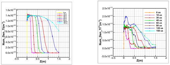
Figure 8.
Variation curves for the number densities of atomic Ti and Ti2+ along the z-direction at different times on the symmetry axis.
After 120 us, the mainstream potential of the flow field gradually approaches zero and is close to the quasi-neutral state. Although the ion number density in the flow field of the small cylinder is high, it continues to decline and gradually approaches the implantation density after 160 us. It is predicted that the flow density in the large cylinder region also increases gradually before finally fluctuating near the injection density, which shows quasi-neutral properties.
Figure 9 shows the variation curves of the atomic Ti and Ti2+ velocities along the z-direction at different times on the symmetry axis. When atomic Ti or Ti2+ does not move to the right-end face, the speed first increases before rapidly decreasing to zero. The particle velocities increase once they break away from the main stream and expand. When particles move to the right-end plane, the main-stream velocity decreases gradually. The atomic Ti velocity decreases after 120 us and the Ti2+ velocity decreases after 60 us, which fully shows that the ion velocity increases rapidly under the action of the electric field. For t > 80 us, the maximum velocity position is out of the simulation domain.
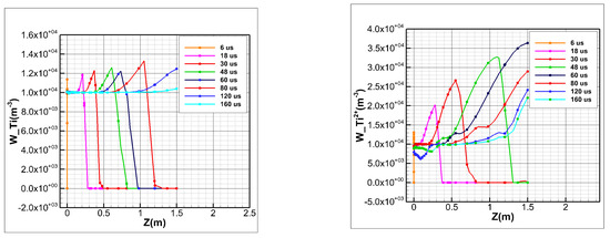
Figure 9.
Variation curves of the atomic Ti and Ti2+ velocities along the z-direction at various times along the symmetry axis.
Figure 10 shows the variation curve of the z-direction velocity along the y-direction at a specific line. At a given time, the velocity first increases and then decreases along the y-direction, which is nearly symmetrical around y = 0 m. At t = 30 us, Ti2+ diffuses near a specific line, and the velocity reaches a maximum. Over time, the velocity at the same position gradually decreases to near the stable value and is gradually stabilized after 60 us. The velocity distribution in the middle is nearly the same and drops rapidly on both sides, reflecting the characteristics of beam flow.
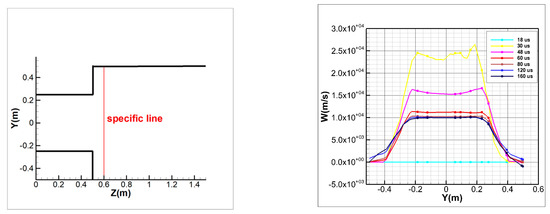
Figure 10.
Variation curves of the z-direction velocity along the y-direction for a specific line.
Figure 11 shows the variation curves of the atomic Ti and Ti2+ number densities along the y-direction for a specific line. The atomic Ti and Ti2+ number densities initially increase and then decrease along the y-direction, which is nearly symmetrical around y = 0. At t = 18 us, atomic Ti does not diffuse near the specific line, but Ti2+ does, indicating that the diffusion speed of Ti2+ under the action of an electric field is faster than that of atomic Ti. Over time, the number density of atomic Ti at the same position gradually increases to near the stable value, which is the injection surface density. The number density increases rapidly near the axis of symmetry and slowly at both ends near the specific line. The Ti2+ number density increases over time near the symmetry axis, slightly exceeds the injection surface density, increases relatively slowly on both sides, and then fluctuates near the injection surface density. At t = 18 us, Ti2+ diffuses near the specific line but has not fully diffused in the y-direction. After t = 60 us, Ti2+ has fully diffused near the specific line.
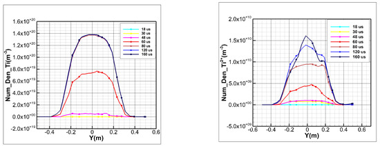
Figure 11.
Variation curves of the atomic Ti and Ti2+ number densities along the y-direction for a specific line.
Figure 12 shows the variation curves of temperature and pressure along the y-direction for a specific line. The temperature variations along the y-direction gradually increase at first, before decreasing and reaching a maximum at the beam edge near the symmetry axis. The temperature near the axis of the flow field gradually increases to a stable value after 48 us. On both sides of the specific line, the temperature gradually begins to fluctuate after 48 us, indicating that the flow begins to reach the edge of the large cylinder. There is a certain particle aggregation near the wall, which results in a gradual increase in the velocity pulsation on both sides of the specific line. Over time, the temperature in the main-stream region increases slowly and the velocity pulsation decreases, while the velocity pulsation increases gradually due to the interactions between the diffusion regions on both sides of the main stream and the particles reflected by the wall. The pressure increases significantly when the high-density region of the small cylinder develops toward the region of the large cylinder. It reaches a stable value after 80 us, and then increases slowly. The distribution of the specific lines is high in the middle and low at both ends, and is symmetrical along y = 0.
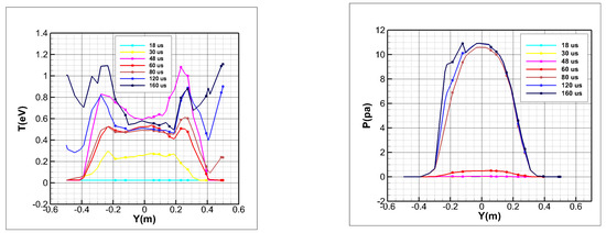
Figure 12.
Variation curves of temperature and pressure along the y-direction on a specific line.
4. Comparison with Experimental Measurements
The plasma mass and energy analyzer (EQP) used in the experiments is shown in Figure 13. The vacuum discharge device uses the displacement platform of the vacuum system to detect the movement of relative particle positions and determine spatial distributions. After entering the mass energy analyzer and reaching the detector end, ions are collected by the secondary electron multiplier. Due to the long distance, it is necessary to determine the ion flight time, which is calculated as approximately tens of microseconds. Considering the ion flight time and discharge pulse width, the pulse generator is used to synchronize the time-matching relationship between the plasma generation and the detector to ensure that the plasma generated via discharge can be completely collected, and that the time-resolved collection of plasma can be achieved.
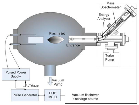
Figure 13.
Schematic diagram of the plasma mass and energy analyzer.
The plasma mass and energy analyzer can only obtain the signal strength at a given energy of one kind of ion by collecting data once for pulsed plasmas. To diagnose the energy distribution, it is necessary to collect experimental data from multiple discharges to obtain the energy distribution curves for different ions. Due to discharge instability, it is necessary to average the data eight times for each data point. The electrode of the pulsed vacuum arc ion source is pure Ti. During vacuum expansion, its valence states are Ti2+, Ti3+, and Ti4+, based on experimental measurements [32]. The ion energy distribution of the plasma plume is measured by the plasma mass and energy analyzer. The energy distributions of ions with various diffusion angles differ. At small deflection angles (α), the energy distributions of Ti2+, Ti3+, and Ti4+ are approximately 90, 90, and 110 eV, respectively. At large deflection angles, the energy distributions are approximately 40, 50, and 50 eV, respectively. This shows that the energy distribution of Ti ions with different valences decreases with the deflection angle.
As there are nearly no collisions between ions in the vacuum expansion, the valence state changes slightly. Three numerical examples were simulated, and their associated components were Ti and Ti2+, Ti and Ti3+, and Ti and Ti4+, respectively. The other conditions were the same as given in Table 1. Table 2 shows the numerical results and the experimental measurements on the specific line (z = 0.6 m) at α = 0°. Figure 14 mainly shows the numerical results for the energy distributions in the axis direction, as represented by α = 0°.
Table 2.
Ion energy for different charge states.
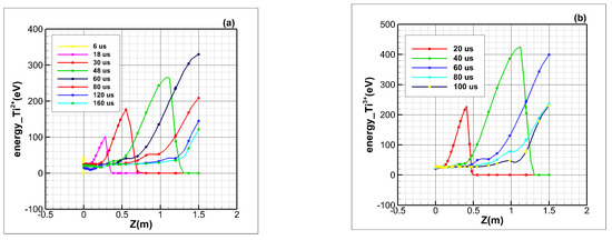
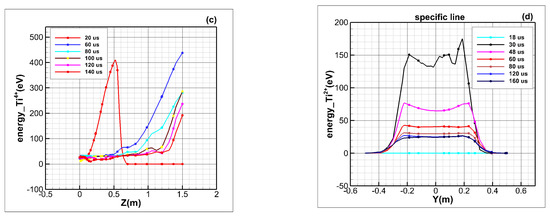
Figure 14.
Ion energy distribution along the central axis of the plasma plume: (a) Ti2+, (b) Ti3+, (c) Ti4+, and (d) Ti2+ (specific line).
The energy distributions on the axis at different times illustrate that when the plasma fills the entire region, the average energy of the particles falls. In the flow field of vacuum expansion, the fastest particles have a much higher velocity and kinetic energy than those near the injection plane. Table 3 demonstrates that the numerical results of average energy are smaller than the EQP measurements, while the smallest and largest velocities are different. Although the plasma charge state changes slightly, the energy of the particles is transformed from kinetic to electric, and the gradient of the self-consistent electric field is larger than the flow field of the unchanged ion charge state assumed by the numerical simulation. It is reasonable to assume that the difference in energy range is caused by the instability of the vacuum arc in the experiment, and the quasi-neutral hypothesis performed in the numerical simulation shows that the electron is not considered as an individual component. The models of the sheath and secondary electron emission will be investigated in future.
Table 3.
Ions’ average energy for different charge states.
The energy distribution for the specific line of Ti2+ shows that when the plasma deflection angle is small, the energy is relatively concentrated. The deflection angle distribution of the experimental data from 0° to 17° is nearly the same as shown in Figure 14, which illustrates that most of the particles are distributed from −0.2 m to 0.2 m. At a certain angle or near y = 0.3 m in Figure 14, the energy decreases rapidly, following the characteristics of beam flow. Penning ion source experiments will be performed using the EQP in future; the measurements of spatial distribution of particles could be compared with numerical simulation results that consider more effects, such as gas–surface interaction, chemical reaction, etc.
5. Parallel Performance Analysis
The simulation domain, meshes, and boundary conditions for electric potentials given in this section are the same as those in Section 4 and as shown in Figure 3. The associated component parameters are shown in Table 4. After 100 timesteps of simulation, the number of simulation molecules was more than 10 million. The simulations were performed on the Tianhe-2 supercomputer.
Table 4.
Hybrid DSMC/PIC algorithm injection parameters.
In order to test the parallel performance of parallel programs, the centralized communication strategy and distributed communication strategy were used. For the same model, parallel computing tests of 24~1536 processes were carried out, and the time consumption and total computing time of the main calculation modules were recorded. The statistical results are shown in Table 5 and Table 6.
Table 5.
Time (unit: s) consumed for parallel computing in the distributed communication strategy.
Table 6.
Time (unit: s) consumed for parallel computing in the centralized communication strategy.
In order to study the performance of parallel computing, the following two parameters were introduced:
- (1)
- Speedup ratio S(p): The speedup ratio refers to the ratio of the total time Ts of the serial algorithm running on a single node to the total time Tp of the parallel algorithm running on multiple nodes for the same computing model; that is:
- (2)
- Parallel efficiency E(p):
Parallel efficiency refers to the ratio of the speedup ratio S(p) of parallel programs to the number of CPUs used. In this study, the number of processes equals the number of CPUs.
The parallel performance of the distributed communication strategy is better than that of the centralized communication strategy. With the same number of processes, the computing time of the distributed communication strategy is significantly less than that of the centralized communication strategy. This is because the distributed communication strategy realizes the direct communication between processes. The process participating in distributed communication can be either the main process or the secondary process, which saves the process of “packaging, transmission, distribution” of information in the calculation process of the centralized communication strategy, reduces the computational cost of parallel communication and, thus, achieves a better acceleration effect.
The efficiency of solving Poisson’s equation is generally not improved with more CPUs. As the number of processes increases, the module time for solving Poisson’s equation increases without decreasing. For the supercomputing platform, the scale of Poisson’s equation solved in this section is small, and the computing communication is relatively low. Therefore, the communication load is dominated when the process is increased, and the scalability of the parallel model is poor, resulting in the computing efficiency being effectively unchanged with the increase in the number of processes.
For the calculation model in this section, the total calculation time using the serial program is 4306.3 s. The distributed communication strategy is more efficient under the current conditions. The speedup ratio and parallel efficiency of the distributed communication strategy are calculated according to Equations (15) and (16), and the results are shown in Table 7.
Table 7.
The speedup ratio and parallel efficiency in the distributed communication strategy.
Parallel computing is significantly faster than serial computing. The speedup ratio reaches 1.91 at 24 processes, and then increases with the number of processes. In the number of processes tested, the maximum speedup ratio (17.94) appears at 768 processes. After that, the speedup ratio decreases. This is because the scalability of parallel computing is not unlimited. When the number of processes is large, the cost of communication between processes is also large. When the computing scale is certain, there is always a maximum acceleration ratio. For the calculation in this section, the maximum acceleration ratio is about 17.94.
The parallel efficiency reaches the maximum value when fully calling 96 processes on a node for calculation, and then continues to decline with the increase in the number of processes. This is because the parallel computing in this section is based on the platform of the Beijing Supercomputing Center. A node has 96 CPUs, which can perform parallel computing for up to 96 processes. When the number of processes is greater than 96, one must manually specify or assign nodes to the platform for calculation. Calling multiple nodes will increase the communication cost between nodes. When the acceleration ratio slows down, the number of CPUs used will increase exponentially. Therefore, the parallel efficiency will decrease when using multiple nodes for calculation.
6. Conclusions
This work used a hybrid DSMC/PIC algorithm employing a combination of Fortran and C++ to realize parallel computing using MPI. The hybrid DSMC/PIC parallel algorithm was investigated to simulate the movement of atomic Ti and Ti2+. The comparative analysis showed that the diffusion speed of Ti2+ under an electric field is faster than that of atomic Ti, especially along the z-direction. The velocities of atomic Ti and Ti2+ first increased before gradually decreasing along the symmetry axis. The electric field accelerated the Ti2+, which moved faster along the main-stream direction. Neutral particles accumulated on the wall due to its fully diffuse reflection model, while charged ions did not—due to their self-consistent electric field. The specific line temperature and pressure were symmetrically distributed. However, after the interactions between the particles and the wall of a large cylinder, the temperature on both sides of the specific line increased, reflecting the influence of interactions between the main stream and the wall. The pressure was observed to change little on both sides of the specific line. The numerical results of average energy were smaller than the EQP measurements, and their range was different. The adoption of the quasi-neutral hypothesis and unchanged charged state failed to simulate the effects of electrons. For the calculation under this study, the maximum acceleration ratio was about 17.94.
Author Contributions
Conceptualization, F.Y.; methodology, F.Y.; software, J.L.; validation, J.L.; formal analysis, D.L., J.L.; investigation, H.Q.; resources, C.X., A.X.; data curation, A.X.; writing—original draft preparation, F.Y.; writing—review and editing, F.Y.; visualization, F.Y.; supervision, J.L.; project administration, J.L.; funding acquisition, J.L. All authors have read and agreed to the published version of the manuscript.
Funding
This research was funded by National Natural Science Foundation of China, grant number [U1730247].
Institutional Review Board Statement
Not applicable.
Informed Consent Statement
Informed consent was obtained from all subjects involved in the study.
Conflicts of Interest
The authors declare no conflict of interest.
References
- Korkut, B.; Li, Z.; Levin, D. Three Dimensional Simulation of Ion Thruster Plumes with Octree Adaptive Mesh Refinement. IEEE Trans. Plasma Sci. 2015, 43, 1706. [Google Scholar] [CrossRef]
- Zhuang, T.; Shashurin, A.; Haque, S.; Keidar, M. Performance characterization of the micro-Cathode Arc Thruster and propulsion system for space applications. Breastfeed. Med. Off. J. Acad. Breastfeed. Med. 2013, 7, 337. [Google Scholar] [CrossRef]
- Choueiri, E.Y. Plasma oscillations in Hall thrusters. Phys. Plasmas 2001, 8, 1411. [Google Scholar] [CrossRef]
- Hirata, Y.; Kato, T.; Choi, J. DLC coating on a trench-shaped target by bipolar PBII. Int. J. Refract. Met. Hard Mater. 2015, 49, 392. [Google Scholar] [CrossRef]
- Taccogna, F.; Minelli, P.; Bruno, D.; Longo, S.; Schneider, R. Kinetic divertor modeling. Chem. Phys. 2012, 398, 27. [Google Scholar] [CrossRef]
- Bird, G.A. Molecular Gas Dynamics; Clarendon Press: Oxford, UK, 1976. [Google Scholar]
- Bird, G.A. Direct simulation and the Boltzmann equation. Phys. Fluids 1970, 13, 2676. [Google Scholar] [CrossRef]
- Pham Van Diep, G.; Erwinand, D.; Muntz, E.P. Nonequilibrium Molecular Motion in a Hypersonic Shock Wave. Science 1989, 245, 624. [Google Scholar] [CrossRef]
- Boyd, I.D. Rotational and vibrational nonequilibrium effects in rarefied hypersonic flow. J. Thermophys. Heat Transf. 1990, 4, 478. [Google Scholar] [CrossRef]
- Everson, J.; Nelson, H.F. Development and application of a reverse Monte Carlo radiative transfer code for rocket plume base heating. In Proceedings of the 31st Aerospace Sciences Meeting, Reno, NV, USA, 11–14 January 1993. [Google Scholar] [CrossRef]
- Plastinin, Y.; Anfimov, N.; Baula, G.; Karabadzhak, G.; Khmelinin, B.; Rodionov, A. Modeling of aluminum oxide particle radiation in a solid propellant motor exhaust. In Proceedings of the AIAA 31st Thermophysics Conference, New Orleans, LA, USA, 17–20 June 1996. [Google Scholar] [CrossRef]
- Hongxia, W.; Liu, D.; Song, Z.; Wang, N.; Yang, C. Monte Carlo Simulation of Laser Transmission Through a Smoke Screen. Chin. J. Comput. Phys. 2013, 30, 415. [Google Scholar]
- Buneman, O. Dissipation of Currents in Ionized Media. Phys. Rev. 1959, 115, 503. [Google Scholar] [CrossRef]
- Eldridge, O.C.; Feix, M. One-Dimensional Plasma Model at Thermodynamic Equilibrium. Phys. Fluids 1962, 5, 1076. [Google Scholar] [CrossRef]
- Hockney, R.W. The gamma network: A multiprocessor interconnection network with redundant paths. J. ACM 1965, 12, 95. [Google Scholar] [CrossRef]
- Dawson, J. One-Dimension Plasma Model. Phys. Fluids 1962, 5, 445. [Google Scholar] [CrossRef]
- Langdon, A.B.; Birdsall, C.K. Theory of Plasma Simulation Using Finite-Size Particles. Phys. Fluids 1970, 13, 2115. [Google Scholar] [CrossRef]
- Zhou, J.; Liu, D.; Liao, C.; Li, Z. CHIPIC: An efficient code for electromagnetic PIC modeling and simulation. IEEE Trans. Plasma Sci. 2009, 37, 2002. [Google Scholar] [CrossRef]
- Scanlon, T.J.; Roohi, E.; White, C.; Darbandi, M.; Reese, J.M. An open source, parallel DSMC code for rarefied gas flows in arbitrary geometries. Comput. Fluids 2010, 39, 2078–2089. [Google Scholar] [CrossRef]
- Wu, J.-S.; Tseng, K.-C.; Wu, F.-Y. Parallel three-dimensional DSMC method using mesh refinement and variable time-step scheme. Comput. Phys. Commun. 2004, 162, 166–187. [Google Scholar] [CrossRef]
- Zhang, Z. Study on Three-Dimensional Plume Flow Field and Pollution Effect of Steady-State Plasma Thruster; University of National Defense Science and Technology: Changsha, China, 2015. (In Chinese) [Google Scholar]
- Copplestone, S.; Ortwein, P.; Munz, C.-D.; Binder, T.; Mirza, A.; Nizenkov, P.; Pfeiffer, M.; Fasoulas, S. Coupled PIC-DSMC Simulations of a Laser-Driven Plasma Expansion. In High Performance Computing in Science and Engineering; Springer International Publishing: Cham, Switzerland, 2016; Volume 15, p. 689. Available online: https://link.springer.com/chapter/10.1007%2F978-3-319-24633-8_44 (accessed on 16 August 2022).
- Shmelev, D.L.; Barengolts, S.; Tsventoukh, M.M. Numerical simulation of plasma expansion at different rates of current rise in the spark stage of a vacuum arc. In Proceedings of the 27th International Symposium on Discharges and Electrical Insulation in Vacuum (ISDEIV), Suzhou, China, 18–23 September 2016; pp. 1–4. [Google Scholar] [CrossRef]
- Revathi, J.; Levin, D.A. CHAOS: An octree-based PIC-DSMC code for modeling of electron kinetic properties in a plasma plume using MPI-CUDA parallelization. J. Comput. Phys. 2018, 373, 571–604. [Google Scholar] [CrossRef]
- Jung, G.; Sung, H.G. Study on Particle Collisions in Hall Thruster Plasma Using a Hybrid PIC-DSMC Mode. Int. J. Aeronaut. Space Sci. 2022, 23, 326–338. [Google Scholar] [CrossRef]
- Li, J.; Yang, F.; Fan, Z.; Du, W.; Xu, A. Numerical Simulation of Axisymmetric Plasma Plume Based on Gas–Surface Interaction/Electric Field Coupling. IEEE Trans. Plasma Sci. 2022, 50, 1097–1112. [Google Scholar] [CrossRef]
- Hughes, T.P.; Hooper, R.W. Boltzmann-Electron Model in Aleph, SAND2014-19974543242; Sandia National Laboratories: Albuquerque, NM, USA, 2014.
- Bird, G.A. Molecular Gas Dynamics and Direct Simulation of Gas Flows; Clarendon Press: Oxford, UK, 1994; pp. 99–146. [Google Scholar]
- Su, Y.; Li, J.; Wang, H.; Xu, A. Numerical Simulation of Chemical Reactions on Rarefied Plasma Plume by DSMC Method. IEEE Trans. Plasma Sci. 2021, 49, 1214–1226. [Google Scholar] [CrossRef]
- Qiu, H.; Xu, C.; Li, D.; Wang, H.; Li, J.; Wang, Z. Parallelizing and Balancing Coupled DSMC/PIC for Large-scale Particle Simulations. In Proceedings of the 2022 IEEE International Parallel and Distributed Processing Symposium (IPDPS), Lyon, France, 30 May–3 June 2022; pp. 390–401. [Google Scholar] [CrossRef]
- Liao, X.; Xiao, L.; Yang, C.; Lu, Y. Milkyway-2 supercomputer: System and application. Front. Comput. Sci. 2014, 8, 345–356. [Google Scholar] [CrossRef]
- Zheng, L. Study on Plasma Parameter Diagnosis of Pulsed Vacuum Arc Ion Source; China Academy of Engineering Physics: Mianyang, China, 2014. (In Chinese) [Google Scholar]
Publisher’s Note: MDPI stays neutral with regard to jurisdictional claims in published maps and institutional affiliations. |
© 2022 by the authors. Licensee MDPI, Basel, Switzerland. This article is an open access article distributed under the terms and conditions of the Creative Commons Attribution (CC BY) license (https://creativecommons.org/licenses/by/4.0/).