Abstract
This paper presents a two-phase guidance and control algorithm to extend the range and improve the impact point accuracy of a 122-mm rocket using a fixed canards trajectory correction fuze. The guidance algorithm consists of a unique glide and correction phase of the rocket trajectory that is activated after the flight’s apex. The glide phase operates in an open-loop configuration where guidance commands are generated to increase the range of the rocket. In contrast, the correction phase operates in a closed-loop configuration where the Impact Point Prediction method based on Modified Projectile Linear Theory is used as a feedback channel to correct the range and drift errors. The proposed fixed canards trajectory correction fuze has a simple and reliable single channel roll-orientation control configuration. The rocket trajectory model consists of a 7-DOF non-linear dynamic model of a dual-spin rocket configuration with a fixed canards correction fuze mounted at the nose. A Monte Carlo simulation of the rocket’s inertial and launch point perturbations show that the fixed canards fuze with the proposed guidance algorithm can double the range of the rocket without changing the rocket motor thrust-time curve. At the same time, the rocket’s accuracy can also be improved beyond the results of an unguided rocket.
1. Introduction
122-mm artillery rockets launched from the Multiple Launch Rocket System (MLRS) are still the first battlefield choice against ground targets, but they are attributed with a short range and larger dispersion radius due to manufacturing inaccuracies and launch-point perturbations. However, modern warfare requires accurate firepower at an extended range to engage a larger target area with minimum repositioning of the launcher so that long-range fire support can be provided for a longer duration. Nevertheless, conventional 122-mm rockets have a maximum range of about 32 km with a target hit accuracy of approximately 500 m. One way to improve its accuracy and extend its range is to design an entirely new precision-guided rocket, but that is an expensive and time-consuming task.
A cost-effective and simple alternative is to add guidance and control features to existing unguided rockets to convert them into guided rockets. With recent technological advancements such as the miniaturization of rugged Micro-Electromechanical System- (MEMS) based inertial sensors, it is currently possible to add guidance and control features into the limited space of a fuze so that it can be retrofitted on to an unguided rocket, converting it into a low-cost, high accuracy guided rocket. Such a fuze system with guidance and trajectory control features is called a trajectory correction fuze. Generally, the control mechanism of these trajectory correction fuzes is implemented through force generated by impulse thrusters or aerodynamic asymmetry caused by cruciform-shaped control canards mounted at the outer surface of the fuze. An impulse thruster-based control mechanism consists of a ring of thrusters mounted near the rocket’s center of gravity, and thrusters provide a short duration impulse force in the radial direction perpendicular to the rocket velocity vector. The canard-controlled trajectory correction fuze falls into two broad categories: one, with moveable canards [1,2,3,4,5]; two, with fixed canards [6,7,8,9]. Moveable canards have multi-channel control and guidance strategies similar to missiles; however, they have the disadvantage of having more moving parts, a complex control mechanism, and high-resolution actuators, resulting, overall, in a higher cost and a lower reliability.
Examples of existing methods for guiding 122-mm rockets include both impulse thrusters and canards. For example, reference [10] describes the use of impulse thrusters for trajectory correction; the author uses the impact point prediction method to calculate deviation from longitudinal and horizontal axes, with the simulation results showing that the Circular Error of Probability (CEP) of uncontrolled rockets = 359 m, while the CEP for general firing control scheme = 38 m, and the CEP for optimum firing control scheme = 20 m. Reference [11] also refers to the 122-mm rocket with 30 thrusters mounted in front of the center of gravity near the nose. The author has used closed-form solutions of linear theory for the impact point prediction guidance algorithm. Monte Carlo simulations for 400 samples show that for unguided trajectory, the CEP = 184.66 m, and while using an impulse thruster force of 1000 n, it claims CEP = 18.87 m. Reference [12] proposes trajectory correction of 122-mm rockets using cyclic control of moveable canards of odd or even numbers. The author has used a guidance scheme based on the impact point prediction method, with the airframe using three canards for correction in a horizontal and vertical frame. The cyclic control of canards generates an average side force and moment similar to the wings of helicopters, 100 Monte Carlo simulations are run, and the results show that an unguided rocket has CEP = 219.05 m and a guided rocket has CEP = 4.25 m.
In comparison to the use of impulse thrusters or moveable canards for 122-mm rocket correction, the fixed canards trajectory correction fuze is a controlled single channel and has the advantage of being simple in design (only one moving part) and, hence, low cost and more reliable. Because of the advantages mentioned earlier, it is natural to use a fixed canards trajectory correction fuze to improve the impact point accuracy of a 122-mm rocket. Whereas to address the issue of extending the range of 122-mm rocket, the conventional method is to alter the rocket motor thrust time curve to increase the rocket motor impulse to achieve maximum burn-out velocity. For example, reference [13] claims that the range can be extended from its existing 20,168 m to 24,443 m with a time delay of 3 s in Thrust-time curve. The other method to increase range is to add impulse thrusters near the rocket’s Center of Gravity (C.G) or, more recently, rocket range can be extended by using high lift ratio moveable canards to increase the angle of attack to generate more lift force [14,15]. However, these methods require a major rocket hardware change, making these methods complex and expensive for the low-cost 122-mm rocket. To summarize, this research proposes a simple, low cost, and reliable fixed canards trajectory correction fuze to both extend the range of 122-mm rockets and improve their accuracy without altering hardware.
The proposed concept of a fixed canards trajectory correction fuze is similar to the Precision Guidance Kit (PGK) that is currently being used for spin-stabilized projectiles [16]. The proposed trajectory correction fuze is mounted on the rocket’s nose like a conventional fuze and is roll-decoupled through a bearing connection. Therefore, the rocket spins due to the roll moment created by canted tail fins, and the correction fuze spins at a low or zero spin rate due to moments created by spin canards. Such a projectile configuration is called a dual-spin projectile with a forwarding control part that spins at a low speed to the spinning aft part [17,18,19,20]. The angles of the correction fuze canards are fixed, which implies that the magnitude of the control force is also fixed; however, the orientation of the control force can be controlled to get the net control force in the desired direction according to the guidance method. This control function is attained through a co-axial servo motor that controls the orientation of this front-mounted correction fuze to get the control force in the desired direction.
The guidance method for such a kind of trajectory correction fuze generally has five types: Trajectory Shaping, Model Predictive Guidance, Trajectory Following, Proportional Guidance, and Impact Point Prediction (IPP). Trajectory Shaping is not suitable when only small corrections are required, whereas the accuracy of Model Predictive Guidance depends on the accuracy of the dynamic model of the projectile and predicted horizon [21,22,23]. Another disadvantage of Model Predictive Guidance is the requirement of an accurate model of the environment and projectile dynamics; it also requires considerable computation time to update the model. In Trajectory Following Guidance, the current position of the projectile are compared with the nominal Trajectory, and control is applied to minimize the error between the current position and nominal position [7]. The disadvantage of Trajectory Following Guidance is that it only uses the current position to correct the trajectory, but it neglects the velocity, which means that the projectile will always try to follow the nominal trajectory and will lose its energy and may fall short of the target. Proportional Guidance is useful in missile guidance, but it is not suitable for ballistic flights, and it has mainly been used with projectiles using jet-thruster correction [24,25]. Finally, Impact Point Prediction (IPP) guidance can be useful for the trajectory correction fuze for small target ranges [26]. The limitation of small ranges can be overcome when the dynamic model of the projectile trajectory is linearized with Modified Projectile Linear Theory [27]. Based on the IPP method, various guidance and control strategies have been studied. An iterative impact point prediction method has been formulated by [28] for fixed canard angle fuze, but this iterative method is not computationally efficient and puts an unnecessary high burden on the guidance computer. Whereas in this research, the impact point is rapidly predicted during discrete intervals of the rocket’s flight using Modified Projectile Linear Theory [29], and control action is based on the swerve response of the projectile, thus eliminating the need for the iterative process. The main reason for using Modified Projectile Linear Theory for IPP is based on the fact that it is more accurate than Projectile Linear Theory and the Modified Point Mass method, and provides accurate results at higher quadrant elevation angles and longer ranges [27]. The proposed guidance method starts after the apex of the trajectory and consists of two guidance phases to maximize the range and reduce the miss-distance errors. The first phase of guidance works to increase the range of the rocket, the so-called Glide Phase; while the second phase of guidance corrects both range and drift errors, the so-called error correction phase.
The main contribution of this research paper is to propose a guidance method that will extend the range of low-spinning fin-stabilized 122-mm rockets with accuracy improvement using a simple, low-cost fixed canards trajectory correction fuze as compared to existing methods of altering rocket motor thrust or by employing impulse thrusters near the rocket’s C.G. Another contribution is a unique two-phase guidance scheme based on the Impact Point Prediction method using Modified Projectile Linear Theory in contrast to conventional predation methods based on the Modified Point Mass method or Projectile Linear Theory. The trajectory simulations of the guided rocket are based on the actual rocket motor thrust-time curve and rocket aerodynamic data fitted with the correction fuze that is realized from the combination of wind tunnel tests and Computational Fluid Dynamics (CFD) simulations.
The paper begins with a description of fixed canards trajectory correction fuze configuration and its 7-DOF dynamic model, along with control authority analysis and, in Section 2, rocket swerve response analysis. Section 3 describes the guidance scheme, Impact Point Prediction method, and Modified Projectile Linear Theory mathematical expressions. Section 4 consists of guided trajectory simulations and a Monte Carlo simulation of 300 samples to investigate the effectiveness of the guidance and control strategy. Finally, Section 5 consists of a discussion of the simulation results.
2. Fixed Canards Trajectory Correction Fuze
The angles of canards mounted on a trajectory correction fuze are fixed and canards are not moveable. Its configuration is shown in Figure 1; it consists of two pairs of fixed canards, i.e., spin canards (1 and 3) and control canards (2 and 4). Spin canards are canted 2° in the opposite direction to produce a counterclockwise roll moment (when viewed from the rear) to overcome rocket spin and roller bearing friction, so the correction fuze can spin in the opposite direction to the main rocket spin. In comparison, the control canards are canted 5° in the same direction to produce a control force and moment perpendicular to the velocity vector of the rocket. When no control is required, the fuze spins freely, so there is no net force in a specific direction; and when control is activated, it produces a control force and control moment in a specific direction. Such a dual-spin projectile configuration can be used to extend the range and correct rocket trajectory errors.
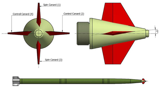
Figure 1.
Correction Fuze Configuration on Rocket.
2.1. 7-Degree of Freedom (DOF) Dynamic Model
The trajectory model of the dual-spin rocket is based on a 7-DOF nonlinear dynamic model expressed in the Body Fixed Plane (BFP) frame as a set of 14 nonlinear differential equations [30]. The dynamic model consists of quaternion rate equations with normalization to determine the Euler Angles of the rocket orientation, so that singularities can be avoided that may occur when the pitch angle of the rocket reaches −90° during the terminal correction phase. The forces and moments acting on the rocket are first converted into the BFP frame before using them in the dynamic model. The 7-DOF dynamic model is numerically integrated using the variable step size fourth-order Runge-Kutta method to increase simulation speed.
The reference frames used in the simulation are Earth Frame, Body Fixed Plane (BFP) Frame, Canard Frame, and Velocity Frame (shown in Figure 2 and Figure 3). The Earth Frame is assumed to be an Inertial Frame with a Flat Earth approximation since the projectile of the trajectory model is a short-range/time of flight rocket, and this approximation has a negligible effect on the accuracy of the results. The BFP frame is similar to Body Frame in a way that, it is rigidly fixed to the rocket’s C.G and exhibits all the linear motions of the rocket, including yawing and pitching motions of the rocket (although it does not roll with the rocket), and its Y-axis always remains in the horizontal plane. The advantage of using the BFP frame lies in the fact that it speeds up the simulation time. The transformation matrix from Canard Frame to BFP Frame (Figure 2), denoted as , is obtained through the rotation of control angle . The transformation matrix from Velocity Frame to BFP Frame (Figure 3) and Canard Frame are and , respectively, and both are acquired after consecutive rotation through the aeroballistics angle of sideslip (−) and angle of attack (), as shown in Equation (1) [30,31].
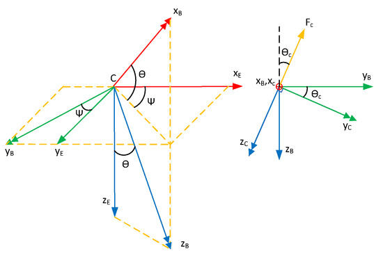
Figure 2.
Earth, BFP and Canard Frame.
Figure 3.
Velocity and BFP Frame.
The dynamic equations of rocket motion expressed in the BFP frame are shown by Equations (2) and (3). The is a diagonal inertia matrix of the rocket containing elements of the principal roll and pitch moment of inertia. The term is the roll rate of the BFP frame required to keep its Y-axis in the horizontal plane.
Here, is the sum of gravity, the aerodynamic forces acting on the rocket, control force generated by canards, gravity force, and rocket motor thrust, all expressed in the BFP frame. The matrix contains the moments contributed from the steady and unsteady aerodynamics of the individual rocket segments. The steady aerodynamics include the moment generated by the rocket body, tail fins, and canards, while the unsteady aerodynamic moments consist of roll and pitch damping moments contributed from the rocket body and tail fins only. All moments are about rocket C.G and are expressed in the BFP frame. Equations (4) and (5) give mathematical expression for calculations of forces and moments in the BFP frame.
The rocket aerodynamic force coefficients appearing in Equation (4) consist of contribution from the zero yaw and squared yaw force coefficients, and are calculated using Equation (6). Similar expressions are also used to calculate canard force coefficients. The zero yaw drag coefficient of the rocket fitted with 0.5° canted tail fins was obtained through wind tunnel tests conducted at Mach numbers from 0.4 to 3.6 according to the test setup of reference [32], while squared yaw coefficients were obtained using CFD simulations.
The turbulence model used in the CFD simulations is based on Reynolds averaged n-S equations, and for the eddy viscosity model, the SST two equation model is adopted. The SST model is also known as the shear stress transport model. The SST model can better improve the accuracy and stability of the numerical simulation of near wall turbulence characteristics based on the standard model. Here, refers to the turbulent kinetic energy, and is the specific dissipation rate (the energy dissipated per unit friction area in unit time). The kinematics of the rocket’s C.G can be expressed using Equation (8) based on quaternions rates Equation (7), owing to their advantage of intrinsic properties.
The yaw and pitch angles are calculated using relationships in Equation (9), whereas the roll rate equation in Body Frame is not directly integrated but is indirectly estimated as a posterior quantity.
The dynamic motion of the trajectory correction fuze is assumed to be perfectly controlled by a servo motor with no lag or overshoot. It is assumed that the servo controller provides the overcoming torque of roller bearing connection, aerodynamic damping moment created by canards, and spin rate along the Xc-axis of the canard frame to keep its Yc-axis always in the horizontal plane. For an ideal case, after compensating for the aforementioned angular dynamics, the angular rate of the canard fuze () measured along the Xc-axis of the canard frame can be considered as zero. The canard fuze orientation is controlled by the control angle (measured from negative Z-axis of BFP Frame); it is calculated by the guidance algorithm to minimize dispersion error.
The main forces in Equation (2) consist of rocket motor thrust, gravity, and aerodynamic forces. The actual rocket motor thrust duration is 3.088 s, measured at sea level (Figure 4). This measured thrust data is adjusted with altitude-based atmospheric pressure at the nozzle exit. The aerodynamic data of the rocket with six straight tail fins (canted at 0.5°) and fixed canards is a combination of wind tunnel test data and CFD simulations that comprise a three-dimensional lookup table as a function of Mach number, angle of attack, and angle of sideslip. The unsteady aerodynamic damping moment coefficients appearing in Equation (5) consist of roll and pitch damping coefficients; these coefficients vary during active motor burning and during passive rocket flight, the coefficients are shown in Figure 5 as a function of Mach number. Figure 6 shows the drag coefficient of the rocket fitted with canards at the various angle of attack and side-slip measured at different Mach numbers; this Drag data also include additional drag induced due to spin and control canards of the correction fuze. Figure 7 shows the normal force coefficient at different Mach numbers for the canards fuze with 5° canted control fins expressed in Velocity Frame. The aerodynamic force coefficients appearing in Equation (4) are measured in the Velocity frame while the moment coefficients appearing in Equation (5) are measured in the body frame, and they need to be transformed into the BFP frame using the transformation matrix (Equation (1) previously used in the dynamic model. The aerodynamic coefficients of a 122 mm rocket without a canard fuze are similar to the data presented in references [12,28,32,33,34,35] which are based on CFD simulations and Missile DATCOM.
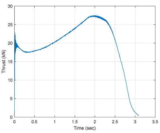
Figure 4.
Rocket Motor Thrust-Time Curve at Sea Level.
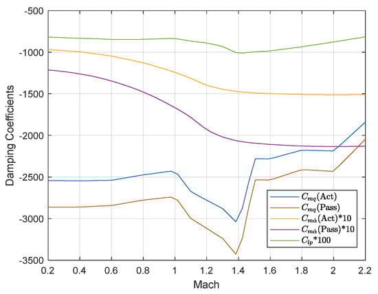
Figure 5.
Damping Coefficients vs. Mach Number.
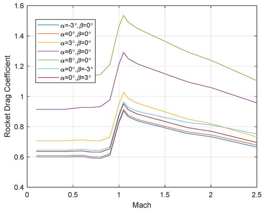
Figure 6.
Drag Coefficient with Correction Fuze.
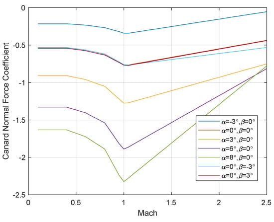
Figure 7.
Canards Normal Force Coefficient.
2.2. Control Authority Analysis
Control Authority analysis is performed to check the correction ability of the trajectory correction fuze when the control angle of the trajectory correction fuze remains fixed in a specific direction in the Body Fixed Plane (BFP) frame (Figure 2). Larger control authority implies the correction fuze’s ability to correct larger perturbations and cover larger areas of engagement.
In this analysis, multiple sets of trajectory simulations are run corresponding to various control activation times and control angles. Each set consists of 72 trajectories with a constant control angle for the entire trajectory selected from an array of 0–355° having a 5° angle step. The simulation results for the control activation times of 90, 95, and 100 s are shown in Figure 8, Figure 9 and Figure 10, respectively. Figure 11 shows the combined impact point footprints of the previously mentioned control activation times. Results show that larger correction ability is obtained when control is activated earlier in the flight (90 s) while smaller correction ability is obtained when control is activated later (100 s) in the flight. For example, when control is activated at 90 s it can achieved ‘range’ control authority from 32 km to 48 km, whereas ‘drift’ control authority of 12 km can be achieved on both sides of the ‘drift’ axis.
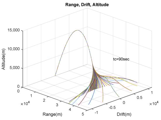
Figure 8.
Control Activated at 90 s.
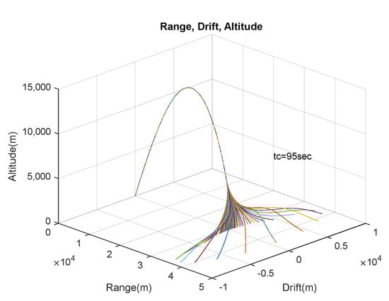
Figure 9.
Control Activated at 95 s.
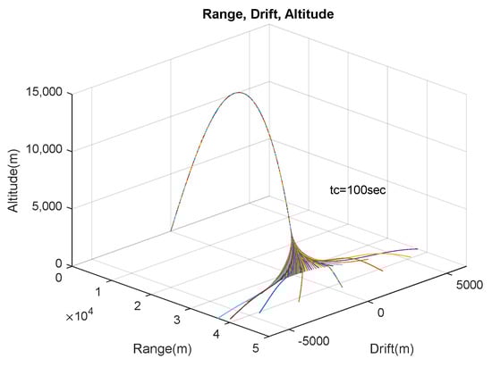
Figure 10.
Control Activated at 100 s.
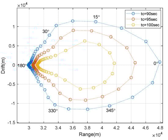
Figure 11.
Foot Print Area.
The footprint area of rocket impact points decreases when control is activated later in the flight. The corresponding area plots of rocket impact points for various control activation times are shown in Figure 11. This area plot is necessary for analyzing and calculating the swerve response of the projectile when control is activated at different intervals of flight.
2.3. Swerve Response
When control force is applied at the nose of a fins-stabilized rocket, the rocket response is not in phase with the control force direction; rather, it responds out of phase with the control force direction due to the coupling of control force, gravity, and gyroscopic effect [17,36]. Therefore, it is important to determine the swerve response of the rocket before implementing the guidance algorithm. The swerve response analysis combines the footprint of rocket impact points of multiple trajectories when the correction fuze control angle () is fixed between 0–360° with 5° step during each trajectory. The output phase angle ∠BAC is calculated from the mean impact point (point A) of rocket impacts, as shown in Figure 12. In this figure, the control is activated at 95 s after launch, and in each simulation, the control angle remains fixed during the entire trajectory, and coordinates of the footprint are measured. In Figure 13, the relationship between control input angle () and response output angle (swerve response) is shown. It is evident that most of the response output is along the range axis towards the launch point, and correction in the drift axis is very sensitive to control input angle. Therefore, a small control input angle can produce a larger correction in the drift axis. The input-output response curve shown in Figure 13 is converted into a cubic polynomial function to be later used in Equation (17) to estimate the control input angle () required for the specific output response direction for trajectory correction.
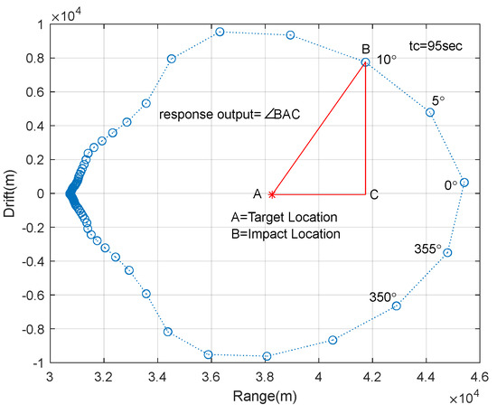
Figure 12.
Footprints of Swerve Response.
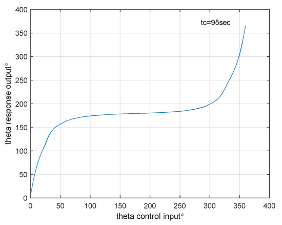
Figure 13.
Swerve Response due to Control Input.
3. Guidance Scheme
The proposed guidance scheme consists of two guidance phases. The first phase of guidance is an open-loop configuration in which the control action is to increase the range of the rocket, therefore called the Glide Phase. While the second phase of guidance works in a closed-loop configuration based on the Impact Point Prediction (IPP) guidance method in which both range and drift errors are corrected using control action. It is assumed that the target coordinates are pre-loaded into the fuze’s guidance computer before launch. Once the guidance is activated, it solves the linear trajectory model based on Modified Projectile Linear Theory and predicts impact coordinates in Earth Frame according to current flight state variables. Then, the control action is generated based on the deviation and orientation of the predicted impact coordinates from the target coordinates. The control action is the orientation of the Trajectory Correction Fuze () to generate control force and moment in a direction to minimize the predicted deviation from the target coordinates. The proposed control law is a unique combination of Impact Point Prediction guidance based on Modified Projectile Linear Theory. The start time of the two guidance phases (i.e., glide and error correction phases) are obtained after the optimization process explained in detail in Section 4.
3.1. Glide Phase
The Glide Phase starts after the apogee of the trajectory with the objective of range enhancement. During this phase, the control angle () of the correction fuze remains fixed in the BFP frame to produce the control force in the upward direction only to increase the range of the rocket. The exact start time of the glide phase after apogee is based on the required target range and launch elevation angle. Thus, the guidance starts earlier for longer target ranges than shorter ones, where the guidance loop starts later in the flight. During the glide phase, the control force and moment due to the canards increases the angle of attack and generates more lift force to compensate for gravity and cause the increase in the range of the rocket.
3.2. Error Correction Phase
Error Correction Phase is a terminal correction guidance scheme based on the Impact Point Prediction (IPP) guidance scheme to calculate the deviation angle from target coordinates (already loaded into correction fuze before flight). The error correction phase is an in-flight iterative process that is invoked after every 0.1 s, during which the impact coordinates of the projectile are predicted using current projectile state variables. The deviation angle (∠BAC) of the predicted impact point from the target is calculated (Figure 12). The control force is required in the direction opposite to the deviation angle, i.e., (∠BAC + π), to correct this deviation angle. For this required control force direction, the control angle of the fuze orientation is calculated from the polynomial swerve function from the swerve response diagram (Figure 13). This calculated control angle is used in the main nonlinear 7-DOF dynamic model, and projectile state variables are updated accordingly.
New coordinates are predicted in the next iteration based on updated projectile state variables, and new control action is generated. This correction process continues until the projectile comes closer to the target location, and errors in range and drift are being removed iteratively. The glide and correction phase process are summarized in the flow chart shown in Figure 14.
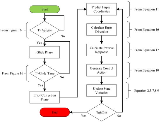
Figure 14.
Guidance Algorithm Flow Chart.
3.3. Impact Point Prediction
The Impact Point Prediction (IPP) method is used as a feedback loop to generate guidance commands to correct trajectory during the error correction phase of rocket flight [12,28,37,38]. The IPP routine is evaluated during the error correction phase after every 0.1 s, making it is a suitable compromise between guidance computation burden and required miss-distance precision. Rapid impact prediction requires a simple analytical model or a linearized trajectory model that a guidance computer can efficiently solve during intermittent flight intervals. Conventionally, the modified point mass method is used as an analytical predictor, or projectile linear theory is used to linearize the trajectory model, but both have limitations and give inaccurate predictions at higher pitch angles and longer ranges. Therefore, Modified Projectile Linear Theory (MPLT) is preferred over other prediction methods since MPLT is still valid at higher pitch angles and longer ranges. Furthermore, it is assumed that the guidance and control unit of the correction fuze contains all the necessary inertial sensors and filtering to obtain full states of projectile trajectory during flight. Rocket position and velocity are calculated using GPS, and rocket Euler Angles are determined by filtered measurements provided by magnetometers.
3.4. Modified Projectile Linear Theory
The Modified Projectile Linear Theory is a set of quasi-linear differential equations written in the BFP frame to predict the future states of the projectile during rapid flight. The time derivative of the trajectory model is changed to the non-dimensional variable ‘s’ arc length, defined as the number of calibers traveled along the trajectory. Moreover, it is assumed that the total velocity slowly varies compared to other variables, that aero-coefficients remain constant during a short interval of time, and that aero-ballistics angles are small enough to be neglected [29]. Integral of Equation (11) provides the coordinates of the predicted impact point in the Earth Frame when the Z-axis changes the sign. These predicted impact coordinates are to be used to generate control action accordingly.
While the epicyclic equations are grouped in a matrix form as follows.
Equations (11)–(15) are numerically integrated using the variable step size fourth order Runge-Kutta method with frozen aerodynamic coefficients to speed up the prediction calculations. The rocket’s predicted impact coordinates (point B in Figure 15) are used to calculate the deviation angle and its magnitude. Correction force is required in the opposite direction (towards D1) of deviation angle to correct deviation Γ. The swerve response of the rocket needs to be adjusted according to the polynomial function defined by Figure 13 using Equations (16) and (17) to get the control force in the required direction.

Figure 15.
Predicted Impact Point Deviation and Magnitude.
4. Simulation Implementation
Numerical simulations are carried out to demonstrate the effectiveness of the proposed guidance scheme to increase the range and accuracy of the 122-mm rocket. The conventional unguided 122 mm rocket has a maximum range of 32 km with the thrust-time curve of Figure 4 and using aero-coefficients of the rocket body without a canard fuze. For the guided simulation scenario, the target point is located at 60 km from the launch point along the range axis, and the rocket is fired at a higher elevation angle of 53° to check the rocket’s stability. Since a larger launch elevation angle may result in rocket instability at the apex of trajectory, and during simulations, it was found out that at 55° launch angle, the subject rocket with a correction fuze tends to become unstable.
An optimization function is formulated to determine the optimized values of the glide phase and the error correction phase start time that gives the minimum value of CEP. The inputs of this function are the start time of the two guidance phases, while the output cost function is the Circular Error of Probability (CEP). Several simulations are run with a sample size of 30 rocket trajectory samples with perturbations, and various combinations of the two-guidance phase start time are investigated. The objective of the optimization function is to find a set of guidance start time values that minimize the cost function. The output plot of the optimization function is shown in Figure 16 with the horizontal axis representing the various glide and error correction phase start times, while the output of the optimization function (vertical axis) is the value of CEP. The contour plot shows that the minimum value of CEP is obtained when the Glide Phase starts at 60 s, and the Error Correction Phase starts at 166 s after launch. Theses optimized values of guidance start times are finalized for guided rocket simulations.
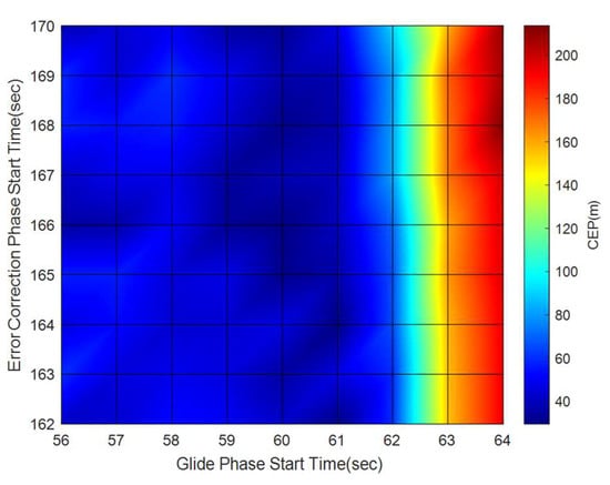
Figure 16.
Guidance Phase Start Time Optimization.
The physical parameters of the 122-mm rocket with initial conditions for simulation are shown in Table 1; these parameters are the nominal values without launch perturbations. The simulation results presented below show that the rocket motor maximum burn-out velocity is 1024 m/s (Figure 17), and that the rocket pitch angle (Figure 18) remains constant during the glide phase while it shows some variations during the terminal error correction phase when the rocket corrects all the drift and range errors. The range plot (Figure 19 and Figure 20) consists of three trajectories: one unguided trajectory without a correction fuze and two guided trajectories with a correction fuze. The two guided trajectories consist of one trajectory with the glide phase only and the second trajectory with both glide and error correction phases. The range plot shows the maximum range of unguided rocket trajectory is 32 km, while plots of guided rocket trajectories show that the guidance algorithm has successfully stretched the rocket trajectory from 32 km to reach the 60 km range during the glide phase. Furthermore, for the error correction phase, the guidance algorithm has efficiently corrected the trajectory with a drift error of only 5 m (Figure 19 and Figure 20), while the other guided rocket without error correction phase has missed the target point with an error of 1150 m. The plots of ballistics angles (Figure 21 and Figure 22) show that the start of the glide phase causes the angle of attack to increase and remain constant to generate more lift. The figure shows that most of the control effort causes the angle of attack to increase in comparison to the side slip; however, both the angle of attack and sideslip remain within limits and show the stability of rocket flight.

Table 1.
Initial Conditions and Error Budgets.
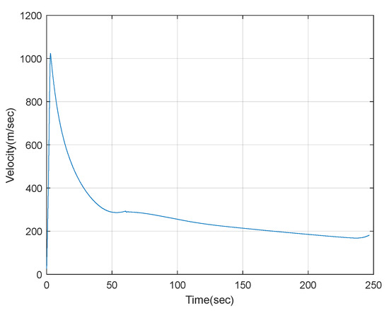
Figure 17.
Velocity Plot.
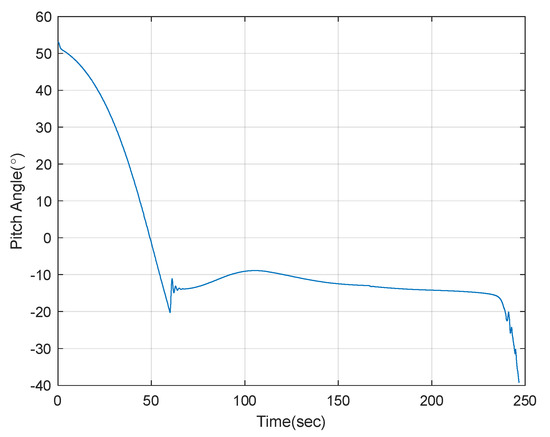
Figure 18.
Pitch Angle.
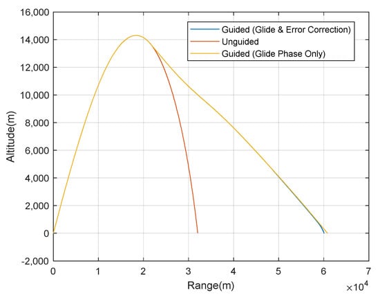
Figure 19.
Altitude vs. Range.
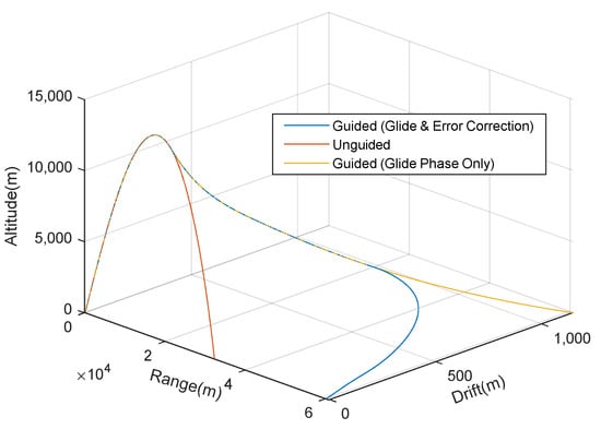
Figure 20.
Altitude vs. Drift vs. Range.
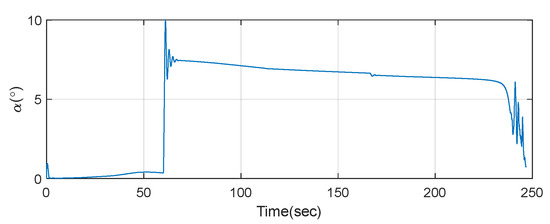
Figure 21.
Angle of Attack.
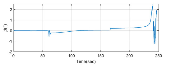
Figure 22.
Angle of Side Slip.
4.1. Perturbation Analysis
A Monte Carlo simulation of 300 samples with Gaussian distributed errors comprising the launch point perturbations and rocket inertial inaccuracies is carried out to establish the effectiveness of the guidance scheme. The target location is 60 km along the range axis. Since the unguided rocket has a range of 32 km, to compare it with a guided rocket, the unguided rocket uses one guidance phase of an open-loop glide phase with the fixed orientation of the correction fuze to increase its range to 60 km. In comparison, the guided rocket has both phases of guidance, i.e., glide phase and error correction phase. In these simulations, a higher quadrant elevation angle is used for both scenarios. The initial conditions and error budgets with gaussian normal distribution are set the same for both simulations, as expressed in Table 1.
4.2. Results and Discussion
Monte Carlo simulation results consist of 300 sample trajectories for unguided (with glide phase only) and guided rockets with perturbations described in Table 1. The Monte Carlo simulation was run in MATLAB R2021a on an Intel Core i5 8th Gen processor laptop with 8 GB of RAM, and it took 6325 s to completely process all 300 samples. The results consist of a plot of range vs. drift vs. altitude, impact coordinates of the rocket at the target point, calculation of the Circular Error of Probability (CEP) based on 50% of the impact points within circle radius criteria, and histograms to show the number of samples and their miss distance.
From the comparison of result plots, it is clear that the two-phase guidance algorithm can increase the range of rocket from 32 km to 60 km (Figure 23 and Figure 24) and improve the accuracy from CEP = 498 m (Figure 25) of the unguided rocket to CEP = 35 m (Figure 26) for guided rockets. It shows the effectiveness of the relatively simple fixed canard trajectory correction method compared to other complex methods of firing impulse thrusters or using moveable canards. The comparison of the histograms (Figure 27 and Figure 28) gives better insight into guidance algorithm effectiveness by representing the number of rocket samples vs. miss distance from the target location. The miss distance histogram of the unguided rocket is shaped like a bell curve with a mean miss distance of approximately 1500 m. Moreover, substantial improvement is seen for the guided rockets since almost 50% of them have a miss distance less than the 50 m from the target that fulfills the error correction capability of the correction fuze since the 122-mm rocket’s lethal radius is about 50 m.

Figure 23.
Unguided Rocket Trajectories.
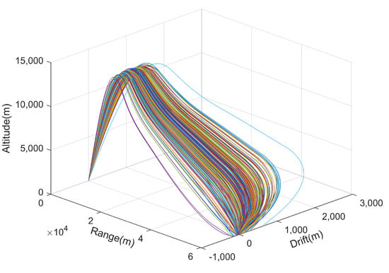
Figure 24.
Guided Rocket Trajectories.
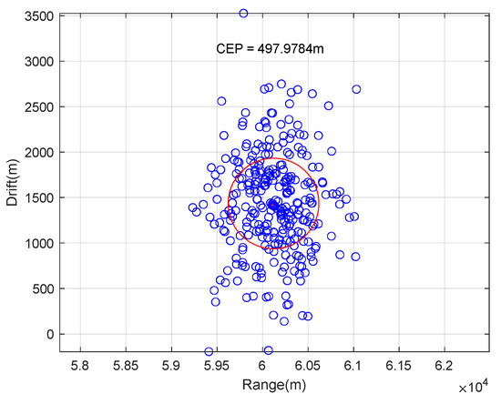
Figure 25.
Unguided Rocket CEP.
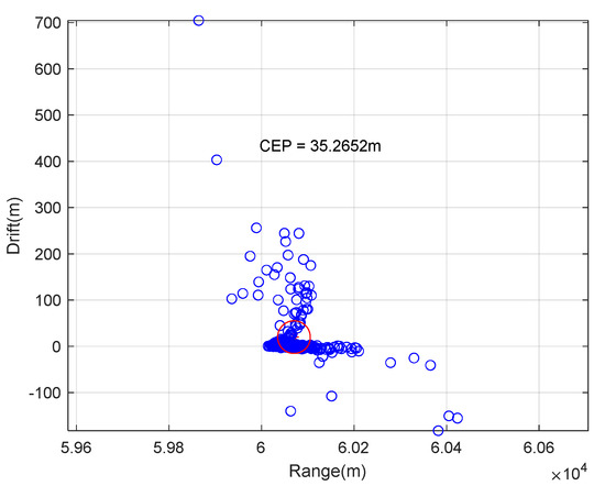
Figure 26.
Guided Rocket CEP.
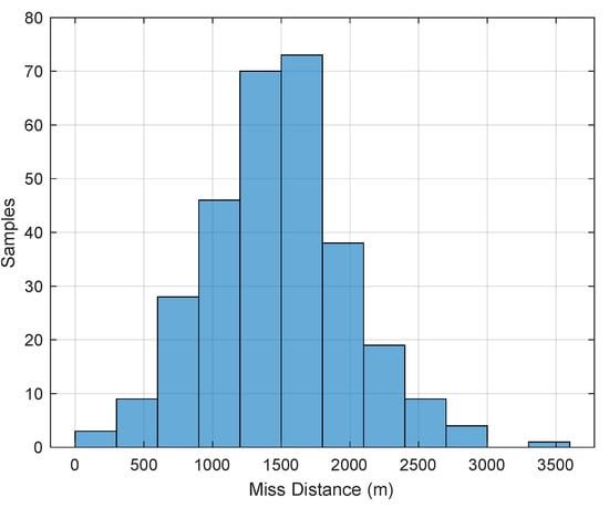
Figure 27.
Unguided Rocket Histogram.
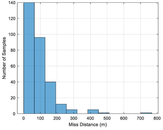
Figure 28.
Guided Rocket Histogram.
5. Conclusions
In this article, a two-phase guidance and control strategy to improve range and accuracy of the 122-mm rocket was presented using a low-cost fixed canards trajectory correction fuze. The trajectory simulations are based on the actual thrust of the 122-mm rocket motor and CFD results. Rocket control authority analysis shows a larger area can be engaged without launcher repositioning, and the rocket does not respond in-phase with the control force direction. Guided rocket simulations show that the proposed two-phase guidance algorithm can increase the rocket range from 32 km to 60 km and also improve the rocket’s target point accuracy. Furthermore, the Monte Carlo simulations were performed to evaluate the effectiveness of the proposed configuration in the presence of perturbations; the results show that the proposed algorithm can reduce the CEP of a guided rocket 14 times more than an unguided rocket, which is a significant improvement.
Author Contributions
Conceptualization, A.R. and H.W.; methodology, A.R.; software and simulation, A.R.; validation, A.R.; formal analysis, A.R. and H.W.; investigation, A.R. and H.W.; writing—original draft preparation, A.R.; writing—review and editing, A.R. and H.W.; visualization, A.R.; supervision, H.W.; project administration, H.W.; funding acquisition, H.W. All authors have read and agreed to the published version of the manuscript.
Funding
This research did not receive any specific grant from funding agencies in the public, commercial, or not-for-profit sectors.
Institutional Review Board Statement
Not applicable.
Informed Consent Statement
Not applicable.
Data Availability Statement
The data, models, and code generated used to support the findings of this study are included within the article.
Conflicts of Interest
The authors declare that there is no conflict of interest regarding the publication of this paper.
Notations
The following symbols are used in this manuscript:
| Earth Frame | Rocket Aerodynamic Force Coefficients in Velocity Frame | ||
| Body Fixed Plane (BFP) Frame | Canard Fuze Aerodynamic Force Coefficients in Velocity Frame | ||
| Canard Frame | Rocket Aerodynamic Moment Coefficients in BFP Frame | ||
| Velocity Frame | Canard Fuze Aerodynamic Moment Coefficients in BFP Frame | ||
| Rocket Velocity in BFP Frame | Zero Drag, Spin, Spin-Damping, Side Force, Normal, and Pitch Damping Coefficients | ||
| Wind Velocities in BFP Frame | Air Density, Characteristic Length, Gravitational Constant, Thrust, Mass | ||
| Rocket Angular Rates in BFP Frame | Dynamic Pressure, Reference Area, Characteristic Length of Projectile | ||
| Quaternion Elements | Distance between Center of Mass and Magnus Center of Pressure | ||
| Euler Role, Pitch, and Yaw Angles | Distance between Center of Mass and Center of Pressure | ||
| Aero-ballistic Angle of Attack and Sideslip | Transformation Matrix from Canard to BFP Frame | ||
| Control Angle input, Orientation of Fuze, and Angular Velocity of Fuze | Transformation Matrix from Velocity to BFP Frame | ||
| Inertia Matrix, Rolling Inertia, Pitch Inertia | Transformation Matrix from Velocity to Canard Frame | ||
| Sum of All forces in BFP Frame | Sum of All Moments in BFP Frame | ||
| Mass of projectile, acceleration due to gravity | Total Velocity along the Trajectory | ||
| Rocket Motor Thrust | Trigonometric Ratio of Subscript Angle |
References
- Rogers, J.; Costello, M. Design of a Roll-Stabilized Mortar Projectile with Reciprocating Canards. J. Guid. Control. Dyn. 2010, 33, 1026–1034. [Google Scholar] [CrossRef]
- Chang, S.; Wang, Z.; Liu, T. Analysis of Spin-Rate Property for Dual-Spin-Stabilized Projectiles with Canards. J. Spacecr. Rockets 2014, 51, 958–966. [Google Scholar] [CrossRef]
- Cooper, G.; Fresconi, F.; Costello, M. Flight Stability of an Asymmetric Projectile with Activating Canards. J. Spacecr. Rockets 2012, 49, 130–135. [Google Scholar] [CrossRef]
- Spagni, J.; Theodoulis, S.; Wernert, P. Flight control for a class of 155 mm spin-stabilized projectile with reciprocating canards. In Proceedings of the AIAA Guidance, Navigation, and Control Conference and Exhibit, Providence, RI, USA, 16–19 August 2004; pp. 1–10. [Google Scholar]
- Theodoulis, S.; Gassmann, V.; Wernert, P.; Dritsas, L.; Kitsios, I.; Tzes, A. Guidance and Control Design for a Class of Spin-Stabilized Fin-Controlled Projectiles. J. Guid. Control Dyn. 2013, 36, 517–531. [Google Scholar] [CrossRef]
- Elsaadany, A.; Wen-Jun, Y. Accuracy improvement capability of advanced projectile based on course correction fuze concept. Sci. World J. 2014, 2014, 273450. [Google Scholar] [CrossRef] [PubMed]
- Gagnon, E.; Lauzon, M. Course Correction Fuze Concept Analysis for In-Service 155 mm Spin-Stabilized Gunnery Projectiles. In Proceedings of the AIAA Guidance, Navigation, and Control Conference and Exhibit, Providence, RI, USA, 16–19 August 2004; pp. 1–21. [Google Scholar]
- Theodoulis, S.; Sève, F.; Wernert, P. Robust gain-scheduled autopilot design for spin-stabilized projectiles with a course-correction fuze. Aerosp. Sci. Technol. 2015, 42, 477–489. [Google Scholar] [CrossRef]
- Clancy, J.A.; Bybee, T.D.; Friedrich, W.A. Fixed Canard 2-D Guidance of Artillery Projectiles. Patent 6,981,672, 3 January 2006. [Google Scholar]
- Gao, M.; Zhang, Y.; Yang, S. Firing control optimization of impulse thrusters for trajectory correction projectiles. Int. J. Aerosp. Eng. 2015, 2015, 781472. [Google Scholar] [CrossRef]
- Jacewicz, M.; Glebocki, R.; Ozog, R. Monte-Carlo Based Lateral Thruster Parameters Optimization for 122 mm Rocket. In Automation 2020: Towards Industry of the Future; Springer: Cham, Switzerland, 2020; pp. 125–134. [Google Scholar]
- Yang, S. Impact-Point-Based Guidance of a Spinning Artillery Rocket Using Canard Cyclic Control. J. Guid. Control Dyn. 2020, 43, 1975–1982. [Google Scholar] [CrossRef]
- Mingireanu, F. Trajectory Modeling of GRAD Rocket with Low—Cost Terminal Guidance Upgrade Coupled to Range Increase Through Step—Like Thrust—Curves. In Proceedings of the 15th International Conference on Aerospace Sciences & Aviation Technology, Cairo, Egypt, 28–30 May 2013; pp. 1–12. [Google Scholar]
- Costello, M. Extended Range of a Gun Launched Smart Projectile Using Controllable Canards. Shock Vib. 2001, 8, 203–213. [Google Scholar] [CrossRef]
- Costello, M.F. Potential Field Artillery Projectile Improvement Using Movable Canards; ARL-TR-1344 Report; US Army Research Laboratory: Aberdeen, MD, USA, 1997; 52p. [Google Scholar]
- Bybee, T. Precision Guidance Kit XM1156. In Proceedings of the 45th Annual NDIA Gun and Missile Systems Conference, Dallas, TX, USA, 17–20 May 2010; Volume 4. [Google Scholar]
- Liu, X.; Li, D.; Shen, Q. Swerving Orientation of Spin-Stabilized Projectile for Fixed-Cant Canard Control Input. Math. Probl. Eng. 2015, 2015, 173571. [Google Scholar] [CrossRef]
- Yin, T.; Jia, F.; Yu, J. Research on Roll Control System for Fixed Canard Rudder of the Dual-Spin Trajectory Correction Projectile. Wirel. Pers. Commun. 2018, 103, 83–98. [Google Scholar] [CrossRef]
- Cheng, J.; Shen, Q.; Deng, Z.; Deng, Z. Novel aiming method for spin-stabilized projectiles with a course correction fuze actuated by fixed canards. Electronics 2019, 8, 1135. [Google Scholar] [CrossRef]
- Zhu, D.; Tang, S.; Guo, J.; Chen, R. Flight stability of a dual-spin projectile with canards. Proc. Inst. Mech. Eng. Part. G J. Aerosp. Eng. 2015, 229, 703–716. [Google Scholar] [CrossRef]
- Fresconi, F.; Ilg, M. Model predictive control of agile projectiles. In Proceedings of the AIAA Atmospheric Flight Mechanics Conference and Exhibit, Honolulu, HI, USA, 18–21 August 2008; American Institute of Aeronautics and Astronautics: Reston, VA, USA, 2012; pp. 1–17. [Google Scholar]
- Letniak, R.; Costello, M. A Nonlinear Model Predictive Observer for Smart Projectile Applications. In Proceedings of the AIAA Atmospheric Flight Mechanics Conference and Exhibit, Honolulu, HI, USA, 18–21 August 2008; Volume 2, pp. 830–850. [Google Scholar]
- Slegers, N. Predictive Control of a Munition Using Low-Speed Linear Theory. J. Guid. Control Dyn. 2008, 31, 768–775. [Google Scholar] [CrossRef]
- Calise, A. An analysis of aerodynamic control for direct fire spinning projectiles. In Proceedings of the AIAA Guidance, Navigation, and Control Conference and Exhibit, Providence, RI, USA, 16–19 August 2004. [Google Scholar]
- Calise, A.J.; El-Shirbiny, H.A.; Kim, N.; Kutay, A.T. An adaptive guidance approach for spinning projectiles. In Proceedings of the AIAA Guidance, Navigation, and Control Conference and Exhibit, Providence, RI, USA, 16–19 August 2004; pp. 3226–3238. [Google Scholar] [CrossRef]
- Fresconi, F. Guidance and Control of a Projectile with Reduced Sensor and Actuator Requirements. J. Guid. Control Dyn. 2011, 34, 1757–1766. [Google Scholar] [CrossRef]
- Fresconi, F.; Cooper, G.; Costello, M. Practical Assessment of Real-Time Impact Point Estimators for Smart Weapons. J. Aerosp. Eng. 2011, 24, 1–11. [Google Scholar] [CrossRef][Green Version]
- ZHANG, X.; YAO, X.; ZHENG, Q. Impact point prediction guidance based on iterative process for dual-spin projectile with fixed canards. Chin. J. Aeronaut. 2019, 32, 1967–1981. [Google Scholar] [CrossRef]
- Hainz, L.C.; Costello, M. Modified Projectile Linear Theory for Rapid Trajectory Prediction. J. Guid. Control Dyn. 2005, 28, 1006–1014. [Google Scholar] [CrossRef]
- Wernert, P.; Leopold, F.; Lehmann, L.; Baer, K.; Reindler, A.; Bidino, D.; Juncker, J. Wind Tunnel Tests and Open-Loop Trajectory Simulations for a 155 mm Canards Guided Spin Stabilized Projectile. In Proceedings of the AIAA Atmospheric Flight Mechanics Conference and Exhibit, Honolulu, HI, USA, 18–21 August 2008; American Institute of Aeronautics and Astronautics: Reston, VA, USA, 2008; pp. 1–18. [Google Scholar]
- Zipfel, P.H. Modeling and Simulation of Aerospace Vehicle Dynamics, 2nd ed.; American Institute of Aeronautics and Astronautics: Reston, VA, USA, 2007; ISBN 978-1-56347-875-8. [Google Scholar]
- Dupuis, A.; Berner, C. Wind tunnel tests of a long range artillery shell concept. In Proceedings of the AIAA Atmospheric Flight Mechanics Conference and Exhibit, Monterey, CA, USA, 5–8 August 2002. [Google Scholar] [CrossRef]
- Li, J.M.; He, G.L.; Guo, H.Y. A Study on the Aerodynamic Characteristics for a Two-Dimensional Trajectory Correction Fuze. Appl. Mech. Mater. 2014, 703, 370–375. [Google Scholar] [CrossRef]
- Tun, N.L.; Thuri, M.; Minnzinoo; Li, Z. Aerodynamic Coefficients Prediction for 122 mm Rocket by Using Computational Fluid Dynamics. IOP Conf. Ser. Mater. Sci. Eng. 2020, 816, 012010. [Google Scholar] [CrossRef]
- Khalil, M.; Abdalla, H.; Kamal, O. Trajectory prediction for a typical fin stabilized artillery rocket. In Proceedings of the Aerospace Sciences & Aviation Technology, Cairo, Egypt, 26–28 May 2009. [Google Scholar] [CrossRef]
- Fresconi, F.; Plostins, P. Control mechanism strategies for spin-stabilized projectiles. Proc. Inst. Mech. Eng. Part G J. Aerosp. Eng. 2010, 224, 979–991. [Google Scholar] [CrossRef]
- Hainz, L.; Costello, M. In flight projectile impact point prediction. In Proceedings of the AIAA Atmospheric Flight Mechanics Conference and Exhibit, Honolulu, HI, USA, 18–21 August 2008; Volume 1, pp. 87–127. [Google Scholar]
- Wang, Z.; Chang, S.-J. Impact Point Prediction and Analysis of Lateral Correction Analysis of Two-Dimensional Trajectory Correction Projectiles. Def. Technol. 2013, 9, 48–52. [Google Scholar] [CrossRef]
Publisher’s Note: MDPI stays neutral with regard to jurisdictional claims in published maps and institutional affiliations. |
© 2022 by the authors. Licensee MDPI, Basel, Switzerland. This article is an open access article distributed under the terms and conditions of the Creative Commons Attribution (CC BY) license (https://creativecommons.org/licenses/by/4.0/).