Abstract
This article deals with aerodynamic and structural calculations of several wing designs to compare the influence of the shape on the lift distribution. Various shapes of wings for the required lift and bending moment were optimized to minimize drag and thereby reduce fuel consumption. One example was a wing with a bell-shaped lift distribution, which was proposed by Ludwig Prandtl and has been forgotten over the years. The first part of the paper focuses on minimization of the wing drag coefficient by a low fidelity method and the results are compared with the CFD calculation with good agreement. In the structural part of the analysis, the inner layout of the studied wings was designed. The structural design, containing elementary wing components and optimization loop, was carried out to minimize weight with respect to panel buckling. From these calculations the weights of wings were obtained and compared. In the last part of this study, an analysis of flight performance of an airplane with presented wings was performed for a selected flight mission. Results indicated that, for the free optimized wing, the fuel saving was about six percent.
1. Introduction
The wing is one of the most important parts of a typical airplane. From the outset, aviators and aircraft designers have tried to find the optimal shape of a wing. Nature was the first, and the main, inspiration for the pioneers of aviation. One of the fathers of aviation, Otto Lilienthal, built his gliders based on bird study. He was convinced that powered flight could be realized emulating bird flight. His work concentrated on ornithopters, despite the fact that the propeller-driven, fixed-wing concept was already known [1]. The flapping of wings, which was imitated by ornithopters, was not widely used further, but other aspects of avian flight appeared useful to explore, as will be discussed below.
The history of modern aerodynamics is closely associated with Ludwig Prandtl, who first formulated the relationships describing the basic aerodynamic behavior of the finite wing. The lifting line theory was developed in the beginning of the 20th century, though the first attempts at theory of the finite wing date back to the late nineteenth century. The first theory explaining the aerodynamics of a finite wing was proposed in 1907 by Frederick W. Lanchester in his book Aerodynamics [1] and by Ludwig Prandtl [2,3]. Prandtl also derived optimal lift distribution for minimum induced drag for a given wingspan, known as elliptical lift distribution, which became a basis for wing design. Later, he described the bell-shaped lift distribution, which produces lower induced drag on the wing with higher wingspan than for classical elliptical lift distribution with respect to the total lift [4].
Similar results were obtained independently by Reimar Horten. He investigated the distribution of induced drag and discovered some peculiarities of designed lift distribution. However, these areas of uncertainty have never been explained. He applied this approach to his gliders. In the following years, Jones achieved 15% induced drag reduction due to 15% larger span compared to the elliptical distribution [5]. He also considered the given lift force and bending moment. Work based on minimizing induced drag, through a change in load distribution, was published by Klein and Viswanathant [6,7]. They derived a solution for the case where the same shear force and bending moment are considered. This was calculated considering wing-span load integration, and resulted in 6% less induced drag and 15% higher wingspan than wings with an elliptical load distribution. Previous work has only looked at the shape of the lift distribution and has not dealt with how this distribution will be realistically achieved. The geometric twist of the wing can be used as an effective way to achieve the prescribed shape of lift distribution. Phillips demonstrated that by twisting a wing of any planform and arbitrary lift coefficient, exactly the same induced drag can be achieved as for an elliptical wing [8]. Prandtl, Jones, Klein and Viswanathant considered bending moment as a surrogate model for the weight of the wing for a given lift at minimum induced drag. A more practical approach is to optimize drag for a required lift coefficient and constrain a bending moment as a limiting structural condition. Pate and German [9] used the wing planform of the Boeing 737 as a case study to demonstrate a drag minimizing procedure in which the bending moment is assumed for different manoeuvre lift coefficients. The result was from 1 to 10% decrease in induced drag. A more complex wing design, based on lifting line theory and gradient optimization with a Lagrangian multiplier, was published by Wroblewski and Ansell [10]. They optimized three trapezoid wings with twist as a design variable to achieve elliptical distribution, and minimal induced and viscous drag, respectively. The wind tunnel measurement results of Reynolds’ number (0.5 × 10⁶) showed a potential reduction in drag of up to 12% for the optimized wings relative to the wing with the elliptical distribution. Oil-flow visualization then demonstrated the beneficial character of the flow separation in the proposed wing versus the elliptical wing, where the same flow separation occurred over the entire wingspan. While many of these classic studies showed an increase in aerodynamic efficiency for the bell-shaped versus elliptical lift distribution at the same bending moments as the model of wing weight [11,12], except for [13], these calculations included only the induced drag component. A more precise determination of wing mass, based on aerodynamic load and calculation of total aerodynamic drag and their effect on flight performance, is currently lacking.
However, the authors were unaware of research that explained the aerodynamic consequences until 2016, when an article by Bowers et al. [14] was published. These researchers rediscovered the bell-shaped lift distribution, its influence on the distribution of the induced angle of attack, and how this affects the way the plane is controlled in a lateral direction. A flight test was also carried out to demonstrate and identify the potential of a wing with a bell-shaped lift distribution for proverse yawing. The link between the bell-shaped load and the flight of birds is also described. The flight of birds in formation aims to reduce the energy needed to fly. It uses the downwash velocity generated by the bird at the front to reduce aerodynamic drag. Analysis of flying pelicans in formation indicates that there is wing overlap [15] which is not optimal for an elliptical load distribution but is optimal for a bell-shaped distribution.
Another context of the bell-shaped lift distribution for avian flight can be seen in dynamic soaring. This is one of the interesting phenomena observed in the flight of birds that can fly over very long distances, such as wandering albatrosses, which are able to fly around 120,000 km per year. The albatross can fly almost without flapping its wings utilizing wind shear [16]. Dynamic soaring can be divided into four periodically repeated phases consisting of windward climb, turn in higher altitude, leeward descent, and lower altitude turn. This cycle finishes approximately at the same initial conditions of flight, but with the gain of distance flown. However, to execute the process of dynamic soaring with minimal energy loss, birds need to execute the turn in the best possible way. For this purpose, to control roll and yaw angle, respectively, the birds twist their wings and thus use proverse yaw. This consequence is of great potential interest for practical purposes for increasing the endurance and range of small UAVs [17].
2. Aerodynamic Design and Evaluation of Wing
This section describes the procedure and computational tools employed to achieve optimal design of wing geometry. In the first part, lifting line theory (LLT) is described as a fast, low fidelity computational method, which takes the influence of induced pressure and the viscous component of drag into account. In the following sub-sections, geometry topology, computational mesh and CFD calculations are described for the purpose of validation of a low fidelity computational method. Following this, an optimization procedure, and aspects such as design parameters, computational conditions, etc., are explained. The last part of this section focuses on the analysis of the results.
2.1. Lifting Line Theory
The first mathematical tool which can estimate aerodynamic behavior of the finite span wing was developed by Ludwig Prandtl [2], published three years later in English translation [3]. An elliptical lift distribution as an optimal solution producing minimum induced drag for a given lift and bending moment was derived there. The analogy between a flow and electromagnetic field is used in LLT. Specifically, the Biot–Savart law is used relating to the velocity produced by a semi-infinite segment of a vortex filament. Prandtl described a vortex scheme as a set of horseshoe vortices, the carrier parts of which lie in a single vortex line connecting the aerodynamic centers of the airfoil. The value of a local vortex Γ(y) equals a sum of all vortices which are going through a local point. The vortex distribution has consequences for the airspeed distribution of the flow field. Each vortex induces downwash velocity in its surroundings and its orientation and magnitude determines the induced angle of attack.
The core characteristic in LLT is the downwash velocity w which can be computed according to the notation described in Figure 1 in each spanwise position y0 by
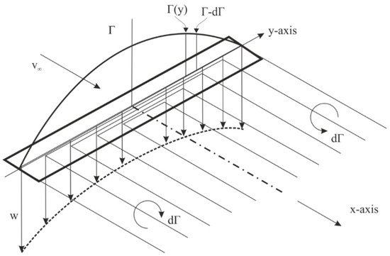
Figure 1.
Spanwise distribution of circulation Γ around the finite span wing and an effect of finite span on downwash velocity w.
The downwash velocity is proportional to the change of circulation and inversely proportional to the geometry of the wing. Unfortunately, circulation is a function of the lift coefficient, and this depends on the induced angle of attack and downwash velocity, respectively. Thus, this equation is in implicit form and must be solved numerically. The calculation process starts with preparation of a geometrical model of the wing-panel distribution. Then, the initial induced angle of attack distribution is estimated (set to zero or adopted from the previous solution). The total angle of attack is computed as a sum of the induced angle of attack , wing angle of incidence and twist angle in the first iteration:
Although lifting line theory is based on a potential flow without a viscosity effect, a stall regime can be estimated through the nonlinearity of two-dimensional airfoil data. Therefore, a local lift coefficient is interpolated from airfoil nonlinear aerodynamic characteristic based on the total angle of attack. The local lift force per unit span depends on air density , air speed , local lift coefficient and local chord , and is computed using the following formula:
Then the Kutta–Joukovsky law is used to determine local circulation:
The computed circulation is then substituted into Equation (1) and a new downwash angle is calculated. If the difference between the computed and initial value is higher than the tolerance, the procedure is repeated until the convergence criteria are satisfied. The total drag is the sum of the induced drag and the airfoil drag, which is also interpolated from the two-dimensional airfoil characteristics. The airfoil drag consists of two parts: pressure and viscous drag. Thus, it is possible to estimate the total wing drag very well.
Three wing configurations were computed and compared with the wind tunnel experimental data to demonstrate the accuracy of the presented computational procedure. Wing geometries are described in the Table 1. Several unswept tapered wings with identical wingspan were defined [18]. The wings had an aspect ratio of 8 (denoted Wing1 in Table 1), 10 (Wing2) and 12 (Wing3), and taper ratio of 2.5. NACA 44-series airfoils of various thicknesses were used. The Reynolds number was approximately 3.5 × 10⁶.

Table 1.
Geometrical characteristics of the wing.
As mentioned above, the accuracy of the two-dimensional aerodynamic characteristics affects the whole computational procedure. In this test case, the aerodynamic airfoil characteristics calculated by the Xfoil program were used. This application showed a good match between the experiment and the calculation for the low-speed regime. A comparison of the LLT computation and the wind tunnel experiment in Figure 2. The same colour for line and maker, respectively, are used for the lift curve and polar characteristics of the corresponding cases. All the wings had quite similar characteristics. The main differences between the wings can be seen in the drag coefficient, which was caused by different aspect ratio and different root airfoils; a higher aspect ratio produces lower induced drag and a thicker airfoil produces higher drag. A reasonable agreement was obtained between the calculated and measured wings. They had almost the same coefficient as measured for linear area, in which the lift coefficient was lower than the maximum lift. The maximum lift coefficient computed was relatively close to the measured value. Moreover, the lift slope, minimum drag and shape of the polar curve were substantially similar.
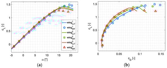
Figure 2.
Comparison of computed (lines) and wind tunnel measured (circles) three wings aerodynamic characteristics. Lift coefficient as function of angle of attack (a) and lift coefficient as function of drag coefficient (b).
2.2. Mesh Generation and CFD Computation
The geometrical sets of the analyzed wings were modelled using the CATIA program, where the sufficiently large cylindrical computational domain was also prepared. Details, including geometrical twist, are provided in Appendix A. Three dimensional geometries were created using polynomial curves describing the distribution of the chord and twist of the profile over the wingspan. For clear analysis, the quarter points of the root profile for all wing platforms were set to the same null coordinate, so that all models had a uniform coordinate system. These geometries served as input for the grid generation in the POINTWISE mesh generator (see Figure 3).
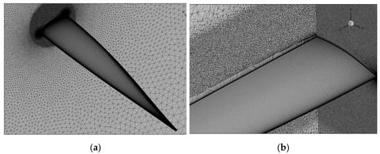
Figure 3.
Surface grid on the wing and the symmetry plane. Prismatic layers and the density region on the symmetry plane can be seen (a). Cross-section of volume grid (b) depicts transition between prismatic layers and outer polyhedral grid. It can be seen that the transition is gradually modeled.
This program is a very powerful and user-friendly tool for various meshing techniques, where the user can easily set needed parameters to create suitable grids for consequent CFD calculation. For the surface mesh, the structured rectangular grid was preferred, but in cases of complex geometry, for example, near the wing tip of an elliptical wing, triangular elements were used. Near the trailing edge, a density region with smooth grid was created to capture aerodynamic effects near the end of the wing (trailing edges had ten elements per trailing edge thickness) and for the better description of the vortex structure. Before the final mesh was generated, the parameters of the volume mesh were set. For the volume grid, tetrahedral elements were used. Approximately 60 prismatic layers were generated to simulate the boundary layer. The wall distance of the first element was set for the desired y+ ≈ 1. This number of layers ensured a sufficiently smooth transition to the volume grid. The total number of elements was approximately 40 million for all computed cases. The number of elements was influenced by the surface mesh and the density region. All computations were performed using the CFD program, m-EDGE [19]. For analyzed wings the compressible Reynolds-averaged Navier–Stokes equations, with W&J EARSM + Hellsten k-omega Turbulence model and a central discretization scheme, was used [20,21]. Results from the CFD calculations were compared with low fidelity methods. Analysis focused on both global aerodynamic characteristics, lift curve, polar curve, maximum lift and drag coefficient, and lift distribution for individual wings. The CFD analysis also provided visualization of fluid flow with the aid of the TECPLOT program. The pressure distribution and vortex structure were investigated to explore agreement with the numerical output.
2.3. Wing Optimization Procedure
The optimization procedure was aimed at minimizing total aerodynamic drag for a given lift force and bending moment. The lifting line theory was used as an optimization tool and two-dimensional aerodynamic characteristics of the selected GAW1 airfoil were calculated in CFD for several Reynolds numbers and angles of attack to cover the whole airfoil regime on the wing. These characteristics were further used in LLT for better prediction of total aerodynamic drag. The designed shape of the wing was calculated using CFD at the end of the optimization process and then these geometries were validated using the high-fidelity method. Different optimization methods were used for different wing planform designs. Most of the wing geometries were optimized by a combination of design of experiment and response surface methods [22]. This approach will be explained in more detail in the next paragraph. Wing geometry without swept and dihedral was considered. The computational conditions are defined in Table 2.
Table 2.
Definition of computational regime.
Three general geometries were optimized in the first stage: rectangular, elliptical, and trapezoidal. The shape of wing geometry was determined by elementary geometrical characteristics, such as wingspan, root and tip chords, or chord distribution, respectively. Another pair of wings were designed in order to investigate the effect of the bell-shaped lift distribution. The first was a wing (BSLS-UTW) with two main design parameters, root chord and wingspan, and an optimization loop calculating the chord distribution to achieve the prescribed load distribution. The second was a trapezoidal wing (BSLS-TW) with three main design parameters, which were the wingspan, the root and the tip chord. The desired bell-shaped load was provided through a wing twist. For the purposes of the internal optimization loop, the control points of the Bezier curve were used to determine the shape of the twist and the chord distribution, respectively. The last wing geometry (FREE-OPT) was generated by two independent distributions of chord and twist that were also created using control points of the Bezier curve. To minimize aerodynamic drag for a given lift and bending moment, the FREE-OPT wing genetic algorithm was used as an optimization method.
All other wings were designed using the RSM which is a method based on fitting the design space and finding the optimum on this surrogate model. In the first steps of this procedure, several randomly selected variants were calculated and are shown by the filled circles in Figure 4. This shows the design space for creating a geometry of a rectangular wing that depends on the span and chord. From the results, the first surrogate model was performed, separately for aerodynamFic drag, and for the bending moment, which is shown in the graph by a dashed line that delimits the set not exceeding the maximum bending moment.
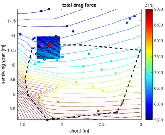
Figure 4.
This picture shows aerodynamic drag for rectangular wing as a function of chord and wingspan. Calculated geometry is labeled by points. Area with maximum bending moment is bordered by dashed lines. Optimal geometry defined by chord and wing is marked by red cross.
In these models, the optimal drag-minimizing geometry was obtained for a given bending moment, which is shown in the graph with a pink “+” sign. In the second step of optimization, a narrow area of optimum was selected from the first step and new variants were calculated on it. From these, a second, more accurate, surrogate model was built, and a new optimization was performed. The narrow area for the second optimization step is shown in the image by color-filled contours and the result of the second step is shown by a red “x” on the chart. It should be noted that RSM was used as a surrogate model, which is based on minimizing the error squares by means of a polynomial approximation, for which the method of least squares is used. To determine the wing drag for a given lift, the aerodynamic polar of the wing was calculated and the desired angle of attack was determined. The wing with the angle of attack, thus defined, was then counted, and the drag and bending moment determined. Calculating a wing polar using a lifting line took several seconds, depending on the number of panels and the calculated angle of attack. The optimization process described above to optimize the rectangular wing of the park takes minutes per row unit. Therefore, this procedure is appropriate for the preliminary aerodynamic wing design. Both the calculation of the lifting line and the optimization processes were created using the MATLAB program.
2.4. Comparison of CFD Results with Low Fidelity Methods
The following series of pictures and graphs depict the comparison of lift distribution of the optimized wing and CFD visualization of individual cases. From the figures of polars on the right side, a good match between the lifting line theory and CFD calculation can be seen, primarily the area of lower lift coefficient that is not affected by a flow separation. Figure 5, left, shows how CFD could help to reveal the structure of vortices. Cross-sections of the volume depict the distribution of the vorticity behind the wing, and the isosurfaces depict the selected value of the Q-criterion. The Q-criterion illustrates areas in the flow field where the vorticity dominates. All the images show the same value of the Q-Criterion 2.15 × 10⁹ and it is possible to compare how much energy is converted into vortex structures and thus aerodynamic drag. From these pictures alone, it is evident that the greatest drag of all the wings studied will be the rectangular wing.
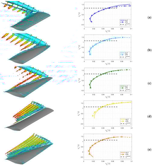
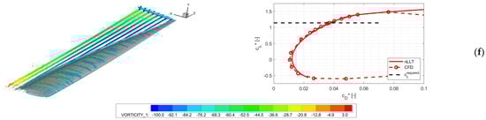
Figure 5.
Visualization of the fluid flow over the wing, cross-section vorticity and Iso-surface Q-criterion (left side); polar diagram—aerodynamic coefficient is related to the reference area (right side). From top to bottom: (a) rectangular, (b) elliptic, (c) trapezoidal, (d) BSLD-TW, (e) BSLD-UTW and (f) FREE-OPT wing.
The x-component of skin friction coefficients can be seen for a higher angle of attack on the left side of Figure 6. Depicted pictures show the behavior of flow near the maximum lift coefficient to better understand the structure of the airflow separation. Places of separated flow are bordered by a black line, which presents zero shear stress where the detachment of the flow starts. The right-hand side of Figure 6 shows the aerodynamic load distribution for both calculation methods, and it is noticeable that, even in this case, there is relatively good agreement between the lifting line theory and CFD at required angles of attack, where the flow was attached. This is a necessary condition for an accurate estimate in the case of the LTT-based method. Note, the wingspan is relative to the rectangular wing. The following series of images illustrate the selected aerodynamic characteristics of calculated wings. Figure 7a depicts different planforms of selected wings. The largest semispan has free optimized wing (red colored planform) followed by wings with bell-shaped distribution. All characteristics and geometry have wingspan related to rectangular wing b/bref which is taken as a reference value.
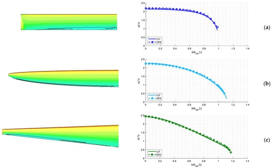
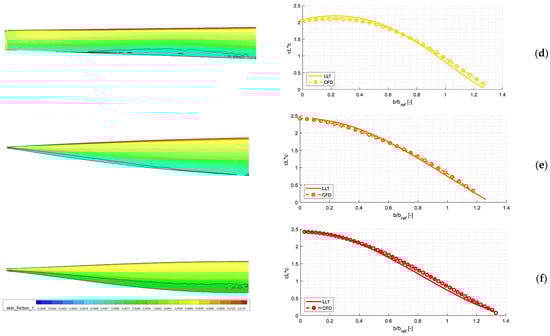
Figure 6.
The x-component of skin friction coefficient on the computed wings. From the calculated polars, a solution was also selected where the detached flow begins to show, approximately two degrees of the angle of attack before maximum lift coefficient is reached. (left side); lift distribution over the wingspan at desired lift force, solid line—lifting line theory, dashed line—CFD (right side). From top to bottom: (a) rectangular, (b) elliptic, (c) trapezoidal, (d) BSLD-TW, (e) BSLD-UTW and (f) FREE-OPT wing.
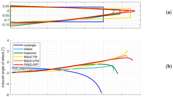
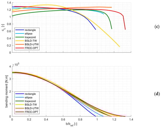
Figure 7.
This series shows a comparison of the aerodynamic characteristics of selected wings. On the picture (a) is depicted geometry of the wings and their different planforms, (b) shows comparison of induced angle of attack, (c) distribution of lift coefficient over the semispan, (d) bending moment coefficient over the semispan.
In Figure 7b, the distribution of induced angle of attack is shown. Wings with bell-shaped distribution have positive value of induced angle of attack near the wing tip, in contrast to other wings. Thus, there is a change of orientation of the induced force vector, based on the analytical equation , to the thrust. In classic wings, the lift distribution is such that it produces only a negative component of the induced angle of attack. Consequently, any control area deflected to produce more lift will also produce more drag. If we consider the deflection of the aileron producing a positive roll moment, it also produces a negative yaw moment, which means a yawing against the turn generated by the rolling motion. This effect is called reverse yaw and is the reason that most aircraft use another control surface, such as rudder, to provide co-ordinate turn without lateral acceleration. For the wing with bell spanwise load, the deflected aileron increases local lift that induces local thrust and thus positive roll moment is connected to positive yaw. This is so-called proverse yaw and was calculated [23] and validated by flight tests [14]. In addition to the advantages of a BSLD on overall drag, the proverse yaw is another phenomenon of this distribution and is probably a missing piece in the analysis of the dynamic soaring that allows migratory birds to fly without mechanical energy over thousands of kilometers [16,24]. Figure 7c shows the lift coefficient distribution. This picture is connected to flow separation and determines where the flow separation begins. For aileron design, it is essential that the flow separation begins at the root section of the wing. The last picture (d) shows that the condition of the same bending moment coefficient is fulfilled.
The next pictures show a comparison of the total aerodynamic drag of wings. The tendency of decreasing aerodynamic drag can be seen in the case of wings with higher aspect ratio, as shown in Figure 8a. The second picture (b) shows polars of optimized wings. The required lift coefficient is indicated as a black dashed line, and the cross of corresponding colors show wing regimes for minimum required power . As can be seen, the rectangular wing experiences the largest distance between minimum power and the target lift. On the other hand, the FREE-OPT wing has the smallest distance between these modes, which can be interpreted as having the best designed wing for given lift under bending moment restriction.
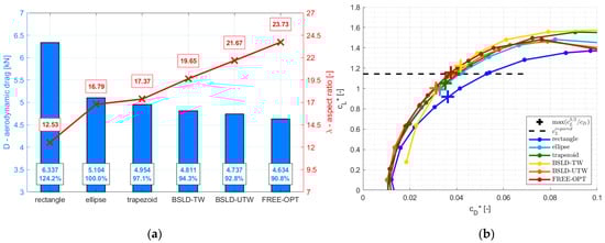
Figure 8.
Image (a) shows comparison of the aerodynamic drag on individual wing with their aspect ratio, (b) shows their polars dashed line labels required lift coefficient, crosses label optimal values of the , which corresponds to minimum required power.
3. Structural Analysis of Wings
In the aerodynamic part of the analysis, the weight of the wing was taken as a function of the bending moment at the root section. This simplified consideration can be taken account of for the analogous geometrical set of tested wings. The aerodynamic analysis provided basic input for following the design of a wing with its elementary elements of construction i.e., spars, ribs, and skin. The inner design of the wing and structural analysis using the MATLAB program were performed again.
The same regime was chosen, as in Table 2, for the load factor n = 2 to determine forces and moments (e.g., shear force, bending and torque moment) acting on the wings considered. In this phase, total mass of the wing was estimated. Other parameters, such as center of gravity, aerodynamic center, and material characteristics, were selected. These data enabled calculation of inertia loads to determine total forces and moments that are distributed to the individual parts of the wing construction. Moreover, construction elements were designed to fulfill structural demands to save weight.
A safety coefficient of 1.5, typical for aircraft design, was set. In this study, the double spar wing was considered, cf. Figure 9. The bending moment was distributed in proportion to the bending stiffness of the individual spars. The structural control of the spar was divided into two parts: flange and web control [25]. The flange was the only structure to transmit bending moment. The upper flange with a larger area transfers pressure and the lower flange is loaded with tension. The area of flange needed to be calculated, such that the stress was less than critical. The local stability was investigated based on the pressure force acting onto the flange, assuming:
where is the bending moment, and is effective height of the spar. A half-restrained variant was considered to determine the critical stress.
Figure 9.
Double spars wing with two cells. This picture serves for shear stress calculation. Sheer fluxes of skin are labeled by , fluxes of spars , describes surface of cell and is thickness of skin or web.
The area of flange was designed by iterative procedure in which the initial size of flange was selected. After that a critical stress was calculated based on empirical relation [25]. In the next step, the stability condition was controlled.
The inner part of the wing was designed as a double spar with two cells, where shear flow in both cells was solved with a set of two equations. These assume that the torque of the first cell equals that of the second one. This statement, together with Bredt’s formula, enables solution of shear flow and controls the function of skin consequently [26]. Figure 9 describes fluxes, forces and moment acting on a two-cells wing.
To calculate the total torque moment, the position of the elastic axis (Figure 9) using the following relation was first determined:
where , are longitudinal elastic moduli of first and second spar and are quadratic cross section moduli for first and second spar.
Spars transmit shear force in ratio of bending stiffness:
where shear is flux of first spar, shear is flux of second spar, is axis force, is length between first and second spar, is distance between the first spar and elastic axis and are heights of the first and respective second spar.
As mentioned above, a set of two equations was calculated for the total fluxes:
where is the total torque moment affecting on cross-section, are areas of first and respective second cell, are fluxes of first and second cells, are lengths of front section of first cell, upper section of the second cell and lower section of the second cell, , are thickness of these sections, are thickness of first and respective second spar, is shear modulus.
While it is necessary to determine two cross-sectional values to calculate the mass of the flanges, it is necessary to determine all the thicknesses shown in Figure 9. to estimate the weight of the skin and spar. For simplicity, we think of , but it is still a system of two equations involving four variables. This problem has been solved numerically to find a solution that complies with Equations (9) and (10), minimizes mass, and satisfies the condition of stability of the individual segments. The stability condition was investigated for the leading-edge panel [27] and for the spars and panels with thickness [27,28]. After the optimization process, the total mass of wings was calculated.
A design velocity of 121.67 ms−1 and load factor n = 2 at altitude 9000 m (ISA) were considered. In contrast to analyses [4,5,6,7,8], where the wing mass was proportional only to the bending moment, the present analytical procedure considered both the bending moment defining the mass of the flanges and the shear force and torque moment that determine the thickness of the webs and skin. This plays a key role in estimating wing mass and as can be seen from Figure 10, the total mass depends on the wing area. Moreover, the difference between the minimum (FREE-OPT) and maximum weight (BLDS-TW) was approximately 205 kg (20%). The estimated wing masses were used in the following simulations to determine flight performance.
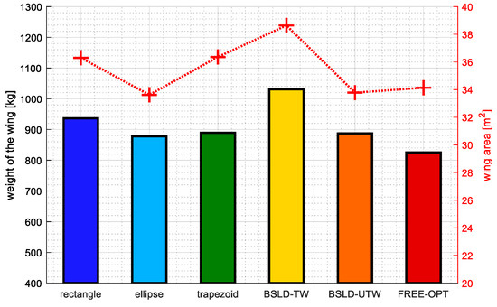
Figure 10.
Estimated weight of the optimized wing.
4. Flight Performance
The most important efficiency parameter of an aircraft is its fuel consumption. For a complex comparison of the characteristics of the individual wings, a flight performance calculation of the flight model example was performed. This consisted of three phases: climb, cruise and glide regimes. The first two regimes contribute to the fuel consumption and the last one determines distance flown in gliding. Each regime was calculated by different equations using aerodynamic characteristics calculated previously with individual mass. To calculate the flight performance of the wing-designed aircraft, it was necessary to estimate the aerodynamic polar for the whole aircraft. For this purpose, a CFD calculation of the whole aircraft with its original geometry was used, where the parts were defined as individual boundary conditions and the results could then separate the aerodynamic forces of the wing and the rest of the aircraft, such as the fuselage, tail surfaces, engine nacelle and landing wheel pods.
The aerodynamic action of these parts may be called parasitic. The polar of the entire aircraft, considered in the flight performance calculations, was then composed of the aerodynamic characteristics of the designed wings and the parasitic part. To predict the impact of the weight of the wing, it was considered that the aircraft with the elliptical wing would have a total design weight of 14,500 kg. The computed performance for the other wings then considered the mass increased by the difference in mass of the chosen wing over the elliptical. For example, the total weight of an aircraft with a BSLD-TW wing was 152.4 kg heavier than an elliptical wing.
4.1. Climb Regime
Climb regime is a flight mode in which the aircraft increases its altitude and increases its potential energy as a result. A steady climb can therefore be characterized as a straight-line flight in a vertical plane, at a constant airspeed. The forces acting on the airplane are described as follows:
where is thrust force, is aerodynamic drag, is aerodynamic lift, is weight of the airplane, is flight path angle, is pitch angle, is angle of attack, and are vertical and horizontal speed, respectively. Vertical speed was determined as 510 [m/min].
4.2. Cruise Regime
Cruise regime is one of the basic flight modes and can be more accurately defined as a straightforward not sideslip flight at a constant speed. Forces acting on the airplane in general horizontal flight are defined by the following equations for lift and drag:
where is the gravitational force that is compensated by the lift of the airplane . This determines the angle of attack required to generate sufficient lift force. Based on the calculated angle of attack is then the drag interpolated from aerodynamic polar and thus thrust is determined. Required power of the aircraft is calculated:
4.3. Glide Regime
For this glide regime the airplane is engine gliding and null fuel consumption is assumed. The forces acting on this aircraft are lift, drag, and weight, the thrust is zero because the power is off. The glide flight path makes an angle γ below horizontal. For an equilibrium unaccelerated glide, the sum of forces must be zero.
where horizontal distance and altitude, is aerodynamic drag, is aerodynamic lift, is weight of the airplane, is flight path angle, is lift-to-drag ratio.
4.4. Total Fuel Consumption
The computation process of total fuel consumption is an iterative process [29]. In the first step the fuel consumption for the climb phase was calculated. Computation of current consumption was performed in every iteration, consequently the decrease of the burned fuel weight was subtracted. With this new weight the next iteration was computed. This approach was used for the climb and cruise phase. Glide (lift-to-drag ratio) determines how far the airplane flies with power off. This phase shortens the cruise phase of flight. Total flying range was 2440 km. The specific power consumption of GE CT7-D engine (considered on L-610) was SFC = 0.274 [kg/(kWh)]. A propeller efficiency to = 85% was estimated. The drag coefficient is a function of lift and was interpolated every time from the actual weight. Weight is decreasing because of fuel consumption. Actual fuel consumption in [kg/s] is:
The basic geometric characteristics of the optimized wings, their aerodynamic drag for given lift and root bending moment, the calculated weights based on stress analysis and the mass of fuel consumed for the mission are shown in Table 3. Calculated using a lifting line theory, the total aerodynamic drag can be divided into parasite (skin friction + pressure drag) and induced drag. The induced drag component is shown in the percentage of the table by the columns of drag D [N]. The wing with the greatest drag, the rectangular wing, had the largest proportion of drag formed by the induced component. In contrast, low-drag wings had a decreasing proportion of the induced component.
Table 3.
Summary of geometrical, aerodynamic, and mass characteristics of wings.
The results of the flight performance are shown in the Figure 11, with total consumption divided for the climb and cruise phases. There was a similarity between wing drag and the fuel consumption of the entire aircraft for the mission. Fuel saving was less than the differences in wing drag as a percentage, which is due to the fact that the fuselage and tail surface drag was taken into account when calculating power and fuel consumption, respectively.
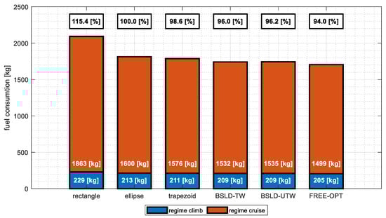
Figure 11.
Comparison of fuel consumption for aircraft with optimized wing; values in the box above the graph determines fuel consumption relative to elliptical wing.
5. Conclusions
Analysis of selected wings with different planform were performed. For the purposes of this study, lift force requirement and root bending moment were given. The aerodynamic analysis revealed a good match between the results of the fast-lifting line method and the CFD calculation, both in terms of total aerodynamic characteristics values and the lift distribution over the semispan. The results confirmed that optimized wings with bell-shaped lift distribution reached smaller drag coefficient values compared to the other wings used. Following this, the structural design for load factor n = 2 under the same flight conditions was performed. The essential elements of inner wing structure, such as web, flange and skin, were optimized to fulfill safety requirements for structural analysis, while achieving the lowest possible mass. The aerodynamic characteristics together with knowledge of mass enabled calculation of flight performance, which showed that, on a simulated flight mission, the aircraft with bell-shaped load distribution can save 4–6% of its fuel consumption compared to an aircraft with the elliptical wing. Moreover, only two optimized wings had favorable lift coefficient distributions from the point of view of aileron function in stall regime, i.e., the rectangular wing and BSLD-TW. However, the rectangular wing had the highest aerodynamic drag and fuel consumption.
It is of note that the selected wings were designed directly for a cruise regime and the wing area did not need to fulfil landing and take-off conditions in terms of minimum speed. This can be exploited for VTOL or distributed electric propulsion, e.g., for aircrafts where the wing is designed for a single mode.
Finally, it is necessary to note the advantages of using the lifting line method with the analytical design of the wing’s structure. It is a fast method that provides solutions within units of seconds and is thus suitable for preliminary wing designs. On the other hand, there are limitations to this approach, because it can only be used to design a wing in regimes where the flow is attached.
Author Contributions
P.H. defined the problem, performed the LTT calculation and optimization process, the design of wings, structural optimization, mass estimation and flight performance. A.D. performed the CFD calculations, extracted and analyzed the data, provided comparison of CFD and LTT calculation, designed and performed the structure analysis of spars, web and skin. A.P. provided consultancy advice during the process and checked the manuscript. All authors have read and agreed to the published version of the manuscript.
Funding
These research activities were carried out from funds provided for the “Long-term development of a research organization” (DKRVO) in the form of institutional support of the Ministry of Industry and Trade of the Czech Republic, IAERO project, sub-project IAERO 4.
Conflicts of Interest
The authors declare no conflict of interest.
Abbreviations
| BSLD | Bell-Shaped Lift Distribution |
| CFD | Computation Fluid Dynamics |
| LTT | Lifting Line Theory |
| RSM | Response Surface Method |
| SFC | Specific Fuel Consumption |
| UAV | Unmanned Aerial Vehicle |
| VTOL | Vertical Take-off |
Appendix A. Geometrical Characteristics of Computed Wings
In the following tables the distribution of chord and the twist of optimized wing geometries over the wingspan are listed.
| Wing Spanwise Position [m] | Local Chord [m] | |||||
| Rectangle | Ellipse | Trapezoid | BSLD-TW | BSLD-UTW | FREE-OPT | |
| 0 | 1.7024 | 1.8024 | 2.3792 | 1.7398 | 2.116 | 1.8772 |
| 0.5 | 1.7024 | 1.8003 | 2.305 | 1.7153 | 2.0739 | 1.8738 |
| 1 | 1.7024 | 1.7954 | 2.2307 | 1.6908 | 2.0319 | 1.866 |
| 1.5 | 1.7024 | 1.7875 | 2.1565 | 1.6663 | 1.9898 | 1.8526 |
| 2 | 1.7024 | 1.7765 | 2.0823 | 1.6418 | 1.942 | 1.8335 |
| 2.5 | 1.7024 | 1.7621 | 2.0081 | 1.6173 | 1.8898 | 1.8088 |
| 3 | 1.7024 | 1.7444 | 1.9339 | 1.5928 | 1.8375 | 1.7787 |
| 3.5 | 1.7024 | 1.723 | 1.8597 | 1.5683 | 1.7817 | 1.7426 |
| 4 | 1.7024 | 1.698 | 1.7854 | 1.5438 | 1.7228 | 1.7007 |
| 4.5 | 1.7024 | 1.6691 | 1.7112 | 1.5193 | 1.6638 | 1.6532 |
| 5 | 1.7024 | 1.6361 | 1.637 | 1.4948 | 1.5976 | 1.6002 |
| 5.5 | 1.7024 | 1.599 | 1.5628 | 1.4703 | 1.5301 | 1.5417 |
| 6 | 1.7024 | 1.5574 | 1.4886 | 1.4458 | 1.4581 | 1.478 |
| 6.5 | 1.7024 | 1.5113 | 1.4144 | 1.4214 | 1.3805 | 1.4094 |
| 7 | 1.7024 | 1.4591 | 1.3402 | 1.3969 | 1.301 | 1.3363 |
| 7.5 | 1.7024 | 1.4015 | 1.2659 | 1.3724 | 1.2175 | 1.2589 |
| 8 | 1.7024 | 1.3366 | 1.1917 | 1.3479 | 1.1327 | 1.1779 |
| 8.5 | 1.7024 | 1.2642 | 1.1175 | 1.3234 | 1.0465 | 1.0935 |
| 9 | 1.7024 | 1.1826 | 1.0433 | 1.2989 | 0.9576 | 1.0065 |
| 9.5 | 1.7024 | 1.0897 | 0.9691 | 1.2744 | 0.8664 | 0.9174 |
| 10 | 1.7024 | 0.9825 | 0.8949 | 1.2499 | 0.7717 | 0.8269 |
| 10.5 | 1.7024 | 0.8549 | 0.8207 | 1.2254 | 0.6736 | 0.7355 |
| 10.6617 | 1.7024 | 0.8079 | 0.7967 | 1.2175 | 0.6414 | 0.706 |
| 11 | - | 0.6967 | 0.7464 | 1.2009 | 0.5734 | 0.6442 |
| 11.5 | - | 0.4776 | 0.6722 | 1.1764 | 0.4717 | 0.5538 |
| 11.8786 | - | 0.1649 | 0.616 | 1.1578 | 0.3931 | 0.4864 |
| 12 | - | - | 0.598 | 1.1519 | 0.3671 | 0.465 |
| 12.5 | - | - | 0.5238 | 1.1274 | 0.2578 | 0.3788 |
| 12.566 | - | - | 0.514 | 1.1242 | 0.2434 | 0.3675 |
| 13 | - | - | - | 1.1029 | 0.1532 | 0.2961 |
| 13.5 | - | - | - | 1.0784 | 0.0557 | 0.2181 |
| 13.53 | - | - | - | 1.0769 | 0.05 | 0.2137 |
| 13.7757 | - | - | - | 1.0649 | - | 0.1779 |
| 14 | - | - | - | - | - | 0.1462 |
| 14.2288 | - | - | - | - | - | 0.1148 |
| Wing Spanwise Position [m] | Local Twist [deg] | |||||
| Rectangle | Ellipse | Trapezoid | BSLD-TW | BSLD-UTW | FREE-OPT | |
| 0 | 0 | 0 | 0 | 4 | 0 | 5 |
| 0.5 | 0 | 0 | 0 | 4.6634 | 0 | 4.998 |
| 1 | 0 | 0 | 0 | 5.2342 | 0 | 4.9767 |
| 1.5 | 0 | 0 | 0 | 5.7171 | 0 | 4.9148 |
| 2 | 0 | 0 | 0 | 6.117 | 0 | 4.8282 |
| 2.5 | 0 | 0 | 0 | 6.4383 | 0 | 4.7247 |
| 3 | 0 | 0 | 0 | 6.6859 | 0 | 4.6079 |
| 3.5 | 0 | 0 | 0 | 6.8645 | 0 | 4.4816 |
| 4 | 0 | 0 | 0 | 6.9786 | 0 | 4.35 |
| 4.5 | 0 | 0 | 0 | 7.0331 | 0 | 4.2167 |
| 5 | 0 | 0 | 0 | 7.0077 | 0 | 4.0843 |
| 5.5 | 0 | 0 | 0 | 6.8604 | 0 | 3.9549 |
| 6 | 0 | 0 | 0 | 6.5874 | 0 | 3.8303 |
| 6.5 | 0 | 0 | 0 | 6.2099 | 0 | 3.7117 |
| 7 | 0 | 0 | 0 | 5.7492 | 0 | 3.5994 |
| 7.5 | 0 | 0 | 0 | 5.2266 | 0 | 3.4938 |
| 8 | 0 | 0 | 0 | 4.6634 | 0 | 3.394 |
| 8.5 | 0 | 0 | 0 | 4.0808 | 0 | 3.2991 |
| 9 | 0 | 0 | 0 | 3.4848 | 0 | 3.2075 |
| 9.5 | 0 | 0 | 0 | 2.7568 | 0 | 3.1164 |
| 10 | 0 | 0 | 0 | 1.8802 | 0 | 3.0235 |
| 10.5 | 0 | 0 | 0 | 0.9022 | 0 | 2.9254 |
| 10.6617 | 0 | 0 | 0 | 0.5677 | 0 | 2.8921 |
| 11 | - | 0 | 0 | −0.1363 | 0 | 2.8178 |
| 11.5 | - | 0 | 0 | −1.1947 | 0 | 2.6967 |
| 11.8786 | - | 0 | 0 | −1.9894 | 0 | 2.5929 |
| 12 | - | - | 0 | −2.2414 | 0 | 2.5569 |
| 12.5 | - | - | 0 | −3.3006 | 0 | 2.3931 |
| 12.566 | - | - | 0 | −3.4469 | 0 | 2.3704 |
| 13 | - | - | - | −4.4608 | 0 | 2.1996 |
| 13.5 | - | - | - | −5.7989 | 0 | 1.9687 |
| 13.53 | - | - | - | −5.8866 | 0 | 1.9525 |
| 13.7757 | - | - | - | −6.6045 | - | 1.8196 |
| 14 | - | - | - | - | - | 1.6897 |
| 14.2288 | - | - | - | - | - | 1.5498 |
References
- Anderson, J.D., Jr. A History of Aerodynamics: And Its Impact on Flying Machines; Cambridge University Press: Cambridge, UK, 1998; ISBN 978-0-521-66955-9. [Google Scholar]
- Prandtl, L. Tragflügeltheorie. I. Mitteilung. Nachrichten von der Gesellschaft der Wissenschaften zu Göttingen, Mathematisch-Physikalische Klasse; 1918; pp. 451–477. Available online: https://gdz.sub.uni-goettingen.de/id/PPN252457811_1918 (accessed on 20 December 2021).
- Prandtl, L. Applications of Modern Hydrodynamics to Aeronautics; NACA Report No 116; NASA: Washington, DC, USA, 1921. [Google Scholar]
- Prandtl, L. Über Tragflügel kleinsten induzierten Widerstandes. In Zeitschrift für Flugtechnik und Motorluftschiffahrt 24 (1933), S. 305–306—Nachdruck in: Gesammelte Abhandlungen zur angewandten Mechanik, Hydro- und Aerodynamik; Springer: Berlin/Heidelberg, Germany, 1961; pp. 556–561. [Google Scholar]
- Jones, R.T. The Spanwise Distribution of Lift for Minimum Induced Drag of Wings Having a Given Lift and a Given Bending Moment; NACA Technical Note 2249; National Advisory Committee for Aeronautics: Washington, DC, USA, 1950. [Google Scholar]
- Klein, A.; Viswanathan, S.P. Minimum Induced Drag of Wings with given Lift and Root-Bending Moment. Z. Für Angew. Math. Phys. ZAMP 1973, 24, 886–892. [Google Scholar] [CrossRef]
- Klein, A.; Viswanathan, S. Approximate Solution of Minimum Induced Drag of Wings with given Structural Weight. J. Aircr. 1975, 12, 124–126. [Google Scholar] [CrossRef]
- Phillips, W.F. Lifting-Line Analysis for Twisted Wings and Washout-Optimized Wings. J. Aircr. 2004, 41, 128–136. [Google Scholar] [CrossRef]
- Pate, D.J.; German, B.J. Lift Distributions for Minimum Induced Drag with Generalized Bending Moment Constraints. J. Aircr. 2013, 50, 936–946. [Google Scholar] [CrossRef]
- Wroblewski, G.E.; Ansell, P.J. Prediction and Experimental Evaluation of Planar Wing Spanloads for Minimum Drag. J. Aircr. 2017, 54, 1664–1674. [Google Scholar] [CrossRef] [Green Version]
- De Young, J. Minimization Theory of Induced Drag Subject to Constraint Conditions; NASA Contractor Report No 3140; NASA: Washington, DC, USA, 1979. [Google Scholar]
- Kroo, I. A General Approach to Multiple Lifting Surface Design and Analysis. In Proceedings of the Aircraft Design and Operations Meetings, San Diego, CA, USA, 31 October–2 November 1984. [Google Scholar] [CrossRef]
- Wakayama, S. and Kroo, I. Subsonic Wing Planform Design Using Multidisciplinary Optimization. J. Aircr. 1995, 32, 746–753. [Google Scholar] [CrossRef] [Green Version]
- Bowers, A.H.; Murillo, O.J.; Eslinger, B.; Technology, J.; Gelzer, C. On Wings of the Minimum Induced Drag: Spanload Implications for Aircraft and Birds; Technical Report Document ID: 20160003578; NASA Armstrong Flight Research Center: Edwards, CA, USA, 2016. [Google Scholar]
- Speeding, G.R. The Wake of a Kestrel (Falco Tinnunculus) in Gliding Flight. J. Exp. Biol. 1987, 127, 45–57. [Google Scholar] [CrossRef]
- Bousquet, G.D.; Triantafyllou, M.S.; Slotine, J.J.E. Optimal Dynamic Soaring Consists of Successive Shallow Arcs. J. R. Soc. Interface 2017, 14, 20170496. [Google Scholar] [CrossRef] [PubMed]
- Mir, I.; Eisa, S.; Maqsood, A. Review of Dynamic Soaring: Technical Aspects, Nonlinear Modeling Perspectives and Future Directions. Nonlinear Dyn. 2018, 94, 3117–3144. [Google Scholar] [CrossRef]
- Neely, R.H.; Bollech, T.V.; Westrick, G.C.; Graham, R.R. Experimental and Calculated Characteristics of Several NACA 44-Series Wings with Aspect Ratios of 8, 10 and 12 and Taper Ratios of 2.5 and 3.5; NACA Report No. 1270; National Advisory Committee for Aeronautics, Langley Aeronautical Lab.: Langley Field, VA, USA, 1947. [Google Scholar]
- Vrchota, P.; Prachař, A.; Hospodář, P. Verification of Boundary Conditions Applied to Active Flow Circulation Control. Aerospace 2019, 6, 34. [Google Scholar] [CrossRef] [Green Version]
- Anderson, J.D. Computational Fluid Dynamics: The Basics with Applications; McGraw-Hill: New York, NY, USA, 1994; ISBN 978-0-07-001685-9. [Google Scholar]
- Anderson, J.D. Introduction to Flight, 6th ed.; McGraw-Hill: New York, NY, USA, 2008; ISBN 978-0-07-126318-4. [Google Scholar]
- Vrchota, P.; Hospodář, P. Response Surface Method Application to High-Lift Configuration with Active Flow Control. J. Aircr. 2012, 49, 1796–1802. [Google Scholar] [CrossRef]
- Hainline, K.; Richter, J.; Agarwal, R.K. Vehicle Design Study of a Straight Flying-Wing with Bell Shaped Spanload. In Proceedings of the AIAA Scitech 2020 Forum, American Institute of Aeronautics and Astronautics, Orlando, FL, USA, 6 January 2020. [Google Scholar]
- Sachs, G.; Traugott, J.; Nesterova, A.P.; Dell’Omo, G.; Kümmeth, F.; Heidrich, W.; Vyssotski, A.L. Flying at No Mechanical Energy Cost: Disclosing the Secret of Wandering Albatrosses. PLoS ONE 2012, 7, e41449. [Google Scholar] [CrossRef]
- Niu, M.C.Y. Airframe Stress Analysis & Sizing, 1st ed.; Technical Book Co: Hong Kong, China; Los Angeles, CA, USA, 1997; ISBN 978-962-7128-07-6. [Google Scholar]
- Megson, T.H.G. Aircraft Structures for Engineering Students, 4th ed.; Elsevier aerospace engineering series; Butterworth-Heinemann: Oxford, UK; Burlington, MA, USA, 2007; ISBN 978-0-7506-6739-5. [Google Scholar]
- Wiedemann, J. Leichtbau: Elemente und Konstruktion; Klassiker der Technik, 3rd ed.; Springer: Berlin/Heidelberg, Germany, 2007; ISBN 978-3-540-33656-3. [Google Scholar]
- Schildcrout, M.; Stein, M. Critical Combinations of Shear and Direct Axial Stress for Curved Rectangular Panels; NACA Report No. 1928; National Advisory Committee for Aeronautics, Langley Aeronautical Lab.: Langley Field, VA, USA, 1949. [Google Scholar]
- Budiansky, B.; Connor, R.W. Buckling Stresses of Clamped Rectangular Flat Plates in Shear; NACA Report No. 1559; National Advisory Committee for Aeronautics, Langley Aeronautical Lab.: Langley Field, VA, USA, 1948. [Google Scholar]
Publisher’s Note: MDPI stays neutral with regard to jurisdictional claims in published maps and institutional affiliations. |
© 2021 by the authors. Licensee MDPI, Basel, Switzerland. This article is an open access article distributed under the terms and conditions of the Creative Commons Attribution (CC BY) license (https://creativecommons.org/licenses/by/4.0/).