Description of a Eulerian–Lagrangian Approach for the Modeling of Cooling Water Droplets

Abstract

The present paper describes a tool developed in-house for the modeling of free-falling water droplet cooling processes. A two-way coupling model is employed to account for the interactions between the droplets and the carrier fluid, following a Eulerian–Lagrangian approach. In addition, a stochastic separated flow technique is employed, involving random sampling of the fluctuating fluid velocity. In physical modeling, two empirical correlations are considered for determining the heat and mass transfer coefficients, with the possibility of accounting for vibrations. The numerical results indicate the preponderance of the interactions between droplet and carrier fluid at various humidity ratios.

1. Introduction

The impact of cooled water droplets and their accretion in lifting surfaces and engine intakes is of paramount importance for safe aircraft operation [1,2,3]. Other areas where cooling phenomena play a preponderant role include refrigeration in the food industry [4], the performance of wind turbines [5] and generally adverse effects related to infrastructures [6].

In order to gain insight into the physical aspects regarding cooling and freezing mechanisms, the present paper describes a Eulerian–Lagrangian approach to modeling the cooling rate of free-falling water droplets. Particles are described following a Lagrangian reference frame, while a finite volume method (FVM) is used for the carrier’s fluid description, corresponding to a Eulerian frame. The interactions between carrier fluid and particles are described following a two-way coupling model, accounting for the increase in particle mass–load ratio.

Eulerian–Lagrangian formulations have seen widespread use in the literature for the modeling of turbulent particle dispersion in dilute flows [7]. There are many reviews dealing with either physical or mathematical aspects of the approach. While Gouesbet and Berlemont [8] and Patankar and Joseph [9] focused on particle-laden and particulate flows, respectively, Subramaniam [10] deals with numerical implementations of Eulerian–Lagrangian approaches for the description of multiphase flows.

In order to study the ice shape and aerodynamic performance of a NACA 0012 airfoil with a heater on the leading edge, Uranai et al. [11] considered the flow field following a Eulerian method, with the droplets’ trajectories computed in a Lagrangian frame. A contribution to a better understanding of the thin ice layer formed behind the heater due to the well-known run-back ice phenomenon was achieved by proving that a modified extended Messinger model based on the work of Messinger [12] was more suitable for de-icing simulations for both rime and glaze ice conditions. Similarly, a computational method based on statistical theory considering a Euler–Lagrange framework was used by Peng et al. [13], in which the effects of turbulent dispersion on water droplet impingement in a NACA 0012 airfoil were considered. This study enhances the predominance of turbulent dispersion in this context, concluding that the deviation of water droplet trajectories and the variation in the impingement coefficient must be considered for geometries in which the turbulent intensity of the flow field near the impinging surface is high.

The study of ice accretion with the purpose of flow control and separation mitigation is also an object of study, as pointed out by Fatahian et al. [14], in which different flap configurations were tested to control flow separation and assess the airfoil aerodynamic performance under hazardous environmental conditions. By coupling the Lagrangian Discrete Phase Model (DPM) and the Eulerian Volume of Fluid (VoF) models in two-dimensional, incompressible and unsteady Reynolds-averaged Navier–Stokes (RANS) equations, they concluded that both rainfall and ice accretion had adverse effects on the airfoil performance, finding additionally that the vortexes grew with a larger size for the coupling of rain and icing conditions, further endangering flying conditions.

Regarding the influence of droplet retention on the ice accretion process, Lian et al. [15] proposed a modified spongy icing model demonstrating the necessity of considering droplet retention on the ice surface when numerically simulating glaze ice accretion, asserting the necessity of accounting for this phenomenon.

Although not usually mentioned as a result of the huge focus on aerodynamic performance, impacts on safe engine operation are also a concern [16,17,18,19,20]. For instance, Norde et al. [21] compared Eulerian and Lagrangian approaches to determine ice-crystal trajectories and impact in a generic turbofan compressor, revealing difficulties in the description of crossing trajectories in the Eulerian approach versus convergence issues for the Lagrangian approach, and stated the necessity of accounting for the interaction between the melting ice crystals and the freezing liquid film and particle re-emission due to liquid film atomization resulting from aerodynamic or centrifugal forces.

An alternative solution for solving these problems is the immersed boundary lattice Boltzmann method [22]. This method uses a regular Eulerian grid for the flow domain and a Lagrangian grid to follow particles in the flow field, using the lattice Boltzmann method for tracking a group of particles and simultaneously providing an alternative to treat the solid–fluid boundary conditions. Nevertheless, the difficulties of this method in the treatment of cases with a complicated boundary and non-structured meshes are usually a drawback.

Overall, developments related to Eulerian–Lagrangian formulations have led to improved descriptions and broadened their application range. For example, Ireland and Desjardins [23] introduced a simple approach to correct the implementation of drag models for systems with two-way coupling, while Ching et al. [24] considered compressible particle-laden flows by suggesting a two-way coupled Eulerian–Lagrangian method for simulating multiphase flows with discontinuous Galerkin schemes on arbitrary curved elements in one- and two-way coupling models.

Traditionally, Eulerian–Lagrangian formulations are classified into either locally homogeneous flow (LFL) or separated flow (SF) models. LFL models assume that the dispersed phase is in local thermodynamic equilibrium with the gas phase, while SF models account for the finite-rate inter-phase transport. For this reason, SF models have received the widest acceptance [25]. The modeling of this inter-phase transport in SF models is achieved through Lagrangian tracking schemes. However, the modeling of these tracking schemes, even though it has been widely addressed, still represents the most significant challenge concerning hybrid Eulerian–Lagrangian formulations.

Gradient diffusion and stochastic separated flow (SSF) models are commonly used to account for the effects of turbulence on droplet dispersion. The first class of models employs empirically derived proportionality constants that resemble the effects observed experimentally, while SSF models, through the specification of a characteristic turbulent eddy lifetime using scaling arguments concerning the turbulence model employed, predict droplets’ dynamics. The discrete random walk model or eddy lifetime model proposed by Gosman and loannides [26] assumes a constant fluctuating velocity component over the particle–fluid interaction time scale, and is usually used in these problems. Nevertheless, other dispersion models in particle-laden flows exist [27].

Eulerian–Lagrangian formulations are commonly encountered in numerical studies dealing with the study of evaporating droplets related to engine fuel consumption [28,29,30]. A three-dimensional computational tool to study turbulent two-phase flows was implemented and tested by Barata [31] and Rodrigues et al. [32] to model the dispersion and evaporation of fuel droplets in two-phase turbulent jets in a cross-flow, characteristic of the conditions encountered in the injector and combustion chambers of aero-propulsive systems. Retaining the original numerical framework, the present work is developed by recasting the thermo-physical formulation from dealing with different fuels to water and the evaporation processes into the description of cooling phenomena. The implemented models, thermodynamic relations and properties of the relevant fluids are discussed throughout the manuscript. Two distinct phases are considered, formulated in a Eulerian–Lagrangian approach, with mass, momentum and energy exchanges. Evidence is found on the role of vibrations and deformations for low relative humidity ratios while at high humidity ratios the impact of these phenomena is lower, suggesting the presence of a transition criterion set at intermediate humidity levels closely related to increasing droplet diameter.

The remainder of the manuscript is organized as follows: first, the governing equations for the gas and droplet fields are described, followed by the thermodynamic relations of the cooling process. Then, the coupling between the considered phases is described, for which the corresponding numerical algorithm is presented. Next, the numerical tests and method validation are addressed, attending first to the influence on the cooling process of a variable droplet diameter considering a constant humidity ratio and then to a variable humidity ratio and a constant droplet diameter. Lastly, conclusions are drawn, taking into account the advantages and limitations of the proposed methodology.

2. Governing Equations

The RANS equations for mass, momentum and energy are considered for an incompressible flow. These equations are written for a stationary, viscous and Newtonian fluid under a conservative form to include source terms that consider mass, momentum and energy exchanges. In addition to these mean flow properties, the mass fraction of the flow is also considered. Reynolds stresses, $\overline{U_i^{\prime }{U}_j^{\prime }}$, are approximated through the eddy viscosity concept and Boussinesq’s hypotheses. Finally, the system of partial differential equations (PDEs) is closed with the $\kappa$–$ϵ$ turbulence model [33] for the determination of the turbulence kinetic energy and its dissipation.

The governing equations can be reduced into a single advective–diffusive conservation equation for a general property per unit volume, $\varphi$, represented in Equation (1), where ${\mathsf{\Gamma }}_{\varphi }$ and $S_{\varphi }$ correspond to the effective diffusion coefficient and the source term for each property, $\varphi$, respectively.

$${\displaystyle \frac{\partial \left(\rho \varphi U_i\right)}{\partial X_i}}={\displaystyle \frac{\partial }{\partial X_i}}\left[{\mathsf{\Gamma }}_{\varphi }{\displaystyle \frac{\partial \varphi }{\partial X_i}}\right]+{\overline{S}}_{\varphi }$$

(1)

The trajectories of representative samples are used to obtain the position and velocity of the droplets. This is achieved by solving the particle momentum equation, according to Newton’s second law of motion via the Eulerian fluid velocity field, which is consequently obtained by solving the RANS equations. Finally, the particle position is represented by an equation that considers both the previous and current locations, the particle velocity and the time it took to travel that distance.

A mathematical expression for the particle motion equation, considering a spherical droplet that accounts for all four types of forces, is suggested by Shirolkar et al. [7]. Nevertheless, in the model employed for cooling free-falling water droplets, only steady-state mechanisms for particle dispersion are considered, resulting in a simplified equation for a three-dimensional Cartesian coordinates system. Equations (2) and (3) respectively represent the new particle position and velocity, with subscript d denoting a droplet property and g a gas field property. The trajectory equations depend directly on three additional parameters: the particle relaxation time, ${\varrho }_d$; the integration time step, $\Delta t$; and the gravitational acceleration, g. The superscripts $NEW$ and $OLD$ correspond to a certain property about the next step and one related to the current one. The parameter $X_i$ and $U_i$ are the generalized position and velocity coordinates.

$$X_{i,d}^{NEW}=X_{i,d}^{OLD}+{\displaystyle \frac{\Delta t}{2}}\left(U_{i,d}^{NEW}+U_{i,d}^{OLD}\right)$$

(2)

$$U_{i,d}^{NEW}=U_{i,g}+\left(U_{i,d}^{OLD}-U_{i,g}\right)e^{-{\displaystyle \frac{\Delta t}{{\varrho }_d}}}+g_i{\varrho }_d\left(1-e^{-{\displaystyle \frac{\Delta t}{{\varrho }_d}}}\right)$$

(3)

The particle relaxation time is defined as the response rate of particle acceleration to the relative velocity between the particle and the carrier fluid, depending on the particle’s inertia and free-fall velocity. This parameter is represented in Equation (4). The parameter d is the droplet diameter, $\rho$ the density, $\mu$ the dynamic viscosity and ${\mathrm{Re}}_{\mathrm{d}}$ the diameter-based Reynolds number.

$${\varrho }_d=\frac{24{\rho }_d{d}^2}{18\mu C_D{\mathrm{Re}}_{\mathrm{d}}}$$

(4)

The droplet drag coefficient, $C_D$, is represented in Equation (5), estimated according to experimental data fitting [34].

$$C_D=\left\{\begin{array}{cc}{\displaystyle \frac{24}{{\mathrm{Re}}_{\mathrm{d}}}}\times \left(1+0.15{{\mathrm{Re}}_{\mathrm{d}}}^{0.687}\right),\hfill & if{\mathrm{Re}}_{\mathrm{d}}<1000\hfill \\ 0.44,\hfill & if{\mathrm{Re}}_{\mathrm{d}}\ge 1000\hfill \end{array}\right.$$

(5)

The remaining two parameters required to solve Equations (2) and (3) are the integration time step and the instantaneous fluid velocity at the particle location differing from the averaged value. For that purpose, a stochastic separated flow (SSF) technique is employed, involving random sampling of the fluctuating fluid velocity from certain known distributions. The SSF technique estimates the fluctuating component of fluid velocity, considering a concept which states that the particle interacts with a succession of eddies as it moves along the computational domain. The fluctuating fluid velocity corresponding to a particular eddy is randomly sampled from a probability density function (PDF) obtained from local turbulence properties. This fluctuating fluid velocity PDF at each particle location is assumed to be a Gaussian, with zero mean and standard deviation equal to $\sqrt{2k/3}$.

The eddy size and lifetime scales needed at each particle location to determine the next interaction time are obtained, resorting to local turbulence properties ($\kappa$ and $ϵ$) along the particle trajectory Kolmogorov time and length scales for isotropic flows. However, when using isotropic SSF models, it is possible to use different expressions for these two turbulence scales [7]. Equations (6) and (7) respectively represent a general expression for the turbulence eddy lifetime time scale, ${\tau }_e$, and length scale, $l_e$. The parameters a and b are two dependent constants, determined either by scaling analysis or from experimental data [7].

$${\tau }_e=a{\displaystyle \frac{k}{\epsilon }}\approx 0.2{\displaystyle \frac{k}{\epsilon }}$$

(6)

$$l_e=b{\displaystyle \frac{k^{3/2}}{\epsilon }}\approx {C_{\mu }}^{3/4}{\displaystyle \frac{k^{3/2}}{\epsilon }}$$

(7)

In addition, the crossing trajectory effect must also be considered, being translated mathematically by the eddy transit time, ${\upsilon }_e$, represented in Equation (8). This parameter is interpreted [26] as the minimum time a particle would take to cross an eddy with a characteristic dimension, $l_e$. It becomes necessary to account for this parameter since a particle may remain trapped inside an eddy for the entire lifetime of that eddy, or may prematurely migrate from one eddy to another before the decay due to the turbulence of the original eddy. This premature migration is usually related to the significant free-fall velocity of the particle under consideration. Thus, if the minimum crossing time calculated is smaller than the eddy lifetime, the particle would jump to another eddy.

$${\upsilon }_e=-{\varrho }_{d}ln\left(1-{\displaystyle \frac{l_e}{{\varrho }_d\Vert U_{i,g}-U_{i,d}\Vert }}\right)$$

(8)

Looking at Equation (8), it becomes clear that there is no solution when the characteristic eddy size is greater than the fluid–particle relative velocity multiplied by the relaxation time. This fact is a consequence of the linearized stopping distance of the particle being smaller than the eddy size, causing the particle to be trapped by the eddy. In this case, the interaction time will be the eddy lifetime. Therefore, the particle will interact with a particular eddy for a time, which is the minimum between the eddy lifetime and the eddy transit time. The fluctuating velocity associated with a particular eddy is assumed to be constant over the interaction time. The time step selected is the eddy–particle interaction time, $t_{int}$, given by Equation (9).

$$t_{int}\approx \Delta t=min\left({\tau }_e,{\upsilon }_e\right)$$

(9)

The fluid velocity sampling and the interaction time make it possible to obtain the particle trajectory from Equations (2) and (3). At the end of each step, a new fluctuating fluid velocity is sampled from a new PDF, generated through local turbulence properties. Consequently, the following interaction time is determined by the local properties at the new particle location.

Concerning the source term, its contribution is divided into a component accounting for the interactions related to the gas field, ${\overline{S}}_{\varphi ,g}$, and the other for the interactions of the droplet field, ${\overline{S}}_{\varphi ,d}$. Equation (10) clarifies the terms that constitute the general source term. Additionally, the contribution of the dispersed phase can also be divided into two contributions calculated for each Eulerian cell of the continuous phase. ${\overline{S}}_{\varphi ,ipt}$ specifies the source term due to inter-phase transport and ${\overline{S}}_{\varphi ,c}$ accounts for the transfer phenomena caused by the cooling phenomenon.

$${\overline{S}}_{\varphi }={\overline{S}}_{\varphi ,g}+\stackrel{{\overline{S}}_{\varphi ,d}}{\overbrace{{\overline{S}}_{\varphi ,ipt}+{\overline{S}}_{\varphi ,c}}}$$

(10)

Table 1. General representation of the system of PDEs, adapted from Gouesbet and Berlemont [8], Sommerfeld [30].

$\mathit{\varphi }$	${\overline{\mathit{S}}}_{\mathit{\varphi },\mathit{g}}$	${\overline{\mathit{S}}}_{\mathit{\varphi },\mathbf{ipt}}$	${\overline{\mathit{S}}}_{\mathit{\varphi },\mathit{c}}$	${\mathsf{\Gamma }}_{\mathit{\varphi }}$
1	-	0	${\sum }_k{\displaystyle \frac{\dot{m_k}{N}_k}{V_{ij}}}$	-
$U_i$	$-{\displaystyle \frac{\partial }{\partial X_i}}\left(p+{\displaystyle \frac{2}{3}}k\right)-{\displaystyle \frac{\partial }{\partial X_j}}{\displaystyle \frac{2}{3}}{\mu }_t{\displaystyle \frac{\partial {\overline{U}}_j}{\partial X_i}}+\rho g_i$	$-{\sum }_k{\displaystyle \frac{\dot{m_k}{N}_k}{V_{ij}}}\left[\left(U_{i,k}^{t+\Delta t}-U_{i,k}^t\right)g_i\Delta t\right]$	${\sum }_k{\displaystyle \frac{\dot{m_k}{N}_k{U}_{i,k}}{V_{ij}}}$	$\mu +{\mu }_t$
T	0	$-{\sum }_k{\displaystyle \frac{N_k}{V_{ij}}}\left(L_{ph}\dot{m_k}+Q_{rel}\right)$	${\sum }_k{\displaystyle \frac{\dot{m_k}{N}_k}{V_{ij}}}{c}_{p,d}\left(T_k\right)T_k$	${\displaystyle \frac{\mu }{\mathrm{Pr}}}+{\displaystyle \frac{{\mu }_t}{{\mathrm{Pr}}_{\mathrm{t}}}}$
${\mathsf{{\rm Y}}}_a$	0	0	0	${\displaystyle \frac{\mu }{\mathrm{Sc}}}+{\displaystyle \frac{{\mu }_t}{{\mathrm{Sc}}_{\mathrm{t}}}}$
${\mathsf{{\rm Y}}}_{wv}$	0	0	${\displaystyle \frac{{\sum }_k\dot{m_k}{N}_k}{V_{ij}}}$	${\displaystyle \frac{\mu }{\mathrm{Sc}}}+{\displaystyle \frac{{\mu }_t}{{\mathrm{Sc}}_{\mathrm{t}}}}$
k	${\mu }_t\left({\displaystyle \frac{\partial {\overline{U}}_i}{\partial X_j}}+{\displaystyle \frac{\partial {\overline{U}}_j}{\partial X_i}}\right){\displaystyle \frac{\partial {\overline{U}}_i}{\partial X_j}}-\rho ϵ$	$\overline{U_j{S}_{U_j,ipt}}-{\overline{U}}_j{\overline{S}}_{U_j,ipt}$	$\overline{U_j{S}_{U_j,c}}-{\overline{U}}_j{\overline{S}}_{U_j,c}+{\displaystyle \frac{1}{2}}{\overline{U}}_j{\overline{U}}_j{\overline{S}}_{\rho }-{\displaystyle \frac{1}{2}}\overline{U_j{U}_j{S}_{\rho }}$	$\mu +{\displaystyle \frac{{\mu }_t}{{\sigma }_k}}$
$ϵ$	${\mu }_t\left({\displaystyle \frac{\partial {\overline{U}}_i}{\partial X_j}}+{\displaystyle \frac{\partial {\overline{U}}_j}{\partial X_i}}\right){\displaystyle \frac{\partial {\overline{U}}_i}{\partial X_j}}\left(C_{ϵ1}{\displaystyle \frac{ϵ}{k}}-C_{ϵ2}{\displaystyle \frac{{ϵ}^2}{k}}\right)$	$C_{ϵ3}{\displaystyle \frac{ϵ}{k}}{\overline{S}}_{k,ipt}$	$C_{ϵ3}{\displaystyle \frac{ϵ}{k}}{\overline{S}}_{k,c}$	$\mu +{\displaystyle \frac{{\mu }_t}{{\sigma }_{ϵ}}}$

summarizes the system of PDEs, where the subscripts t, a and $wv$ respectively indicate properties related to turbulence, dry air and water vapor. ${\mathrm{Sc}}_{\mathrm{d}}$ and ${\mathrm{Pr}}_{\mathrm{d}}$ are the Schmidt and Prandtl numbers. $\mathsf{{\rm Y}}$ is the mass fraction, T the temperature, p the pressure, V the volume, m the mass, N the number of particles, $Q_{rel}$ the relative rate of heat transfer, $L_{ph}$ the latent heat of phase change and $c_p$ the specific heat capacity at constant pressure. The turbulence model constants are defined as $C_{\mu }$ = 0.09, $C_{ϵ1}$ = 1.44, $C_{ϵ2}$ = 1.92, $C_{ϵ3}$ = 1.1, ${\sigma }_{\kappa }$ = 1.0 and ${\sigma }_{ϵ}$ = 1.3.

Cooling Process

The cooling process of water droplets has been studied by different authors over the years [35,36,37,38,39,40,41]. In the present work, a basic heat balance model is used to obtain the rate at which the temperature of a droplet varies over time, assuming that the particle integrates a thermodynamic system in which heat transfer takes place from the droplet to the surrounding environment and vice versa. The heat transfer rate is given by Equation (11), assuming that the droplets’ internal motion is so vigorous that complete mixing is achieved. The effects of vibrations and deformations on the particle are neglected. The surface area is represented by A and the parameters $q_h$, $q_m$ and $q_r$ respectively denote the heat fluxes (per unit area) due to convective heat and mass transfer, and thermal radiation. $h_h$ is the convective heat transfer coefficient, $h_m$ the convective mass transfer coefficient, e the emissivity and $\sigma$ the Stefan–Boltzmann constant of radiation.

$${\displaystyle \frac{d{T}_d}{dt}}={\displaystyle \frac{-A_d}{{\rho }_d{V}_d{c}_{p,d}}}\left(\stackrel{q_h}{\overbrace{h_h\left(T_d-T_{g,\infty }\right)}}+\stackrel{q_m}{\overbrace{L_{ph}{h}_m\left({\rho }_{wv}-{\rho }_{g,\infty }\right)}}+\stackrel{q_r}{\overbrace{e\sigma \left(T_d^4-T_{g,\infty }^4\right)}}\right)$$

(11)

In terms of the convention used, the heat fluxes due to the convective heat transfer and thermal radiation have an outward flux to the surrounding environment. However, since we are undergoing a cooling process, the heat flux due to convective mass transfer has an inwards movement. As a result, a diffusive–convective region occurs around the droplet due to significant temperature variations between the droplet and the far-field region of the gas. The temperature in this area is determined by a combination of the droplet and gas temperatures, and is referred to as a reference temperature.

The values of the convective heat and mass transfer coefficients are usually obtained by considering correlations based on empirical data. When considering the steady-state heat transfer of solid spheres, the Ranz–Marshall correlations [42,43] of Equation (12) are used. They are based on the dimensionless Nusselt (${\mathrm{Nu}}_{\mathrm{d}}$) and Sherwood (${\mathrm{Sh}}_{\mathrm{d}}$) numbers, as functions of Reynolds (${\mathrm{Re}}_{\mathrm{d}}$), Schmidt (${\mathrm{Sc}}_{\mathrm{d}}$) and Prandtl (${\mathrm{Pr}}_{\mathrm{d}}$) numbers.

$$\left\{\begin{array}{c}{\mathrm{Nu}}_{\mathrm{d}}=2+0.6{\mathrm{Re}}_{\mathrm{d}}^{1/2}{\mathrm{Pr}}_{\mathrm{d}}^{1/3}\hfill \\ {\mathrm{Sh}}_{\mathrm{d}}=2+0.6{\mathrm{Re}}_{\mathrm{d}}^{1/2}{\mathrm{Sc}}_{\mathrm{d}}^{1/3}\hfill \end{array}\right.$$

(12)

Additionally, we consider the Ranz–Marshall corrected formulation [44] of Equations (13), which introduces the effects of vibrations and deformations into the computations, whose range of validity is given according to Equation (14).

$$\left\{\begin{array}{c}{\mathrm{Nu}}_{\mathrm{d}}=2+15{\mathrm{Re}}_{\mathrm{d}}^{1/2}{\mathrm{Pr}}_{\mathrm{d}}^{1/3}{\left(\frac{z}{d}\right)}^{-0.7}\hfill \\ {\mathrm{Sh}}_{\mathrm{d}}=2+15{\mathrm{Re}}_{\mathrm{d}}^{1/2}{\mathrm{Sc}}_{\mathrm{d}}^{1/3}{\left(\frac{z}{d}\right)}^{-0.7}\hfill \end{array}\right.$$

(13)

$$3\mathrm{m}\mathrm{m}\le d\le 6\mathrm{m}\mathrm{m};10\le \frac{z}{d}\le 600$$

(14)

The thermodynamic relations needed to obtain the previous relations as well as the thermophysical properties of dry air and water are presented, respectively, in Appendix A and Appendix B.

3. Numerical Algorithm

3.1. Coupling of Continuous and Dispersed Phases

To obtain a converged solution for both phases, it is necessary to couple them. For that purpose, the iterative procedure described in Algorithm 1 is followed. In order to reach convergence, a comparison between the source terms of the previous and current iteration is necessary.

The velocities are evaluated at the cell’s edge in a staggered grid configuration for pressure–velocity coupling, discretized following the Quadratic Interpolation for Convective Kinematics (QUICk) scheme [45]. The Semi Implicit Method for Pressure–Linked Equations (SIMPLE) algorithm [46] is used for the pressure–velocity coupling. Lastly, the system of equations is solved through the Tridiagonal Matrix Algorithm (TDMA).

Algorithm 1: Iterative procedure for the two-way coupling of the dispersed and continuous phases.

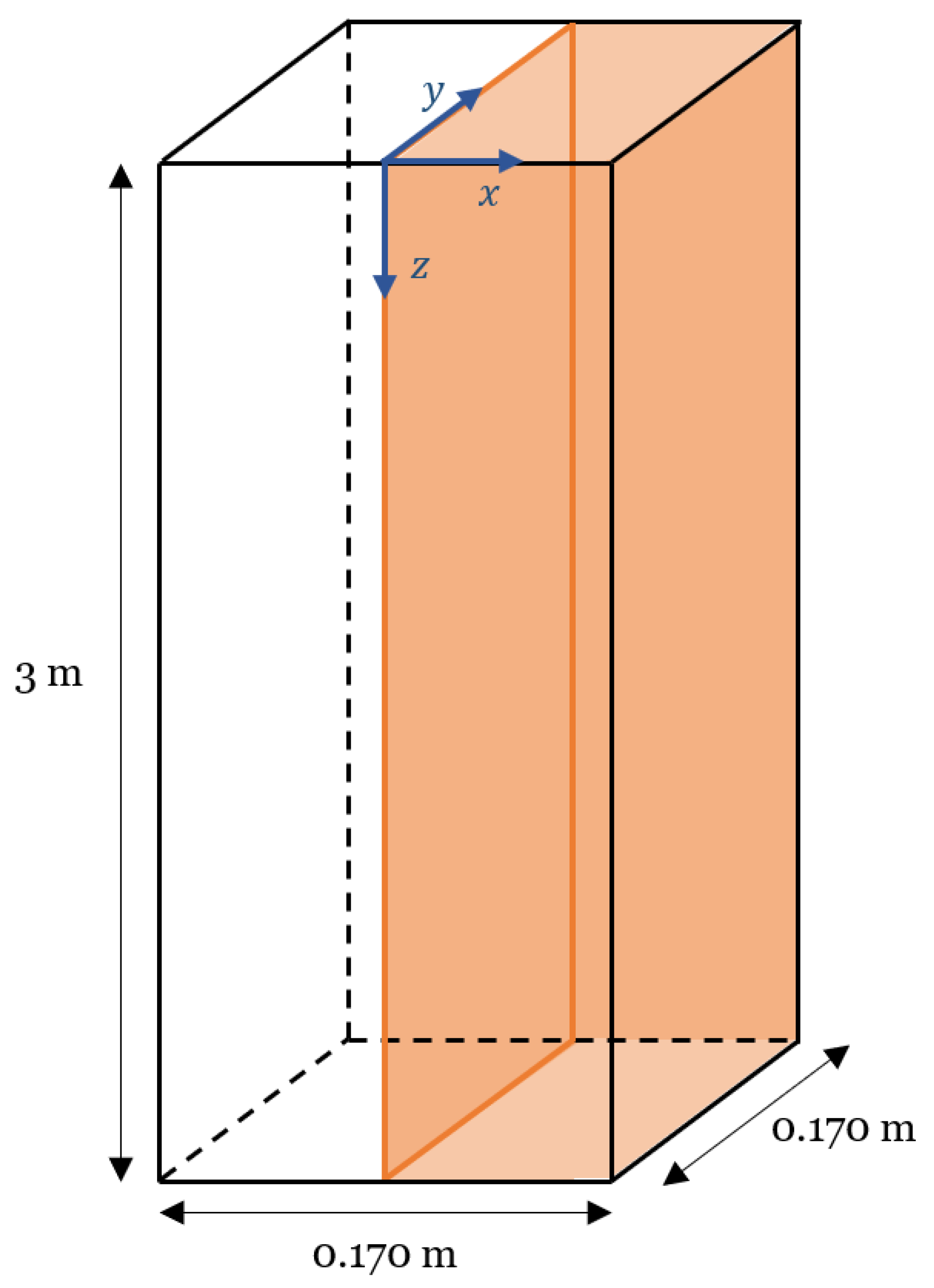
3.2. Initial and Boundary Conditions

We used the experimental conditions of Yao and Schrock [44] to validate the numerical predictions, and they are summarized in

Table 2. Experimental test matrix [44].

Droplet Diameter ($\mathbf{m}\mathbf{m}$)	Relative Humidity Ratio (-)	Initial Droplet Temperature ($\mathbf{K}$)	Environment Temperature ($\mathbf{K}$)
3	$0.29$	$313.85$	$296.44$
3	$0.36$	$313.88$	$295.47$
3	$1.00$	$313.84$	$296.48$
4	$0.36$	$313.89$	$295.59$
4	$0.52$	$313.79$	$294.48$
4	$1.00$	$313.94$	$296.48$
5	$0.29$	$313.83$	$296.03$
5	$0.36$	$313.87$	$295.71$
5	$1.00$	$313.89$	$296.76$
6	$0.36$	$313.89$	$295.29$
6	$0.52$	$313.81$	$294.48$
6	$1.00$	$313.85$	$296.48$

.

The experimental setup consisted of a plastic column of a squared base with a $0.170$ $\mathrm{m}$ edge, 3 $\mathrm{m}$ height and a droplet generator. The droplet generator was set on the center of the upper face and, an air stream was injected downwards from the upper into the lower face with a constant velocity of $0.03$ $\mathrm{m}$/$\mathrm{s}$.

In this way, four distinct droplet diameters (3, 4, 5 and 6 $\mathrm{m}$$\mathrm{m}$) and four different humidity ratios ($0.29$, $0.36$, $0.52$ and $1.00$) were considered. For each droplet diameter, three distinct humidity ratios were used to represent a low, medium and high humidity content.

The computational domain is described in Figure 1. A symmetry plane was considered at $x=0$, resulting in only half the domain being considered. As seen in the figure, the Cartesian reference frame has its origin on the upper face. An inlet was considered on the top face, where the variables were specified with uniform profiles according to the experimental conditions. In the lower plane, an outlet was considered where the normal gradients of the dependent variables were set to zero, and the remaining boundaries were defined as no-slip walls. Lastly, the initial integration interval was of 5 × 10⁻⁵ $\mathrm{s}$.

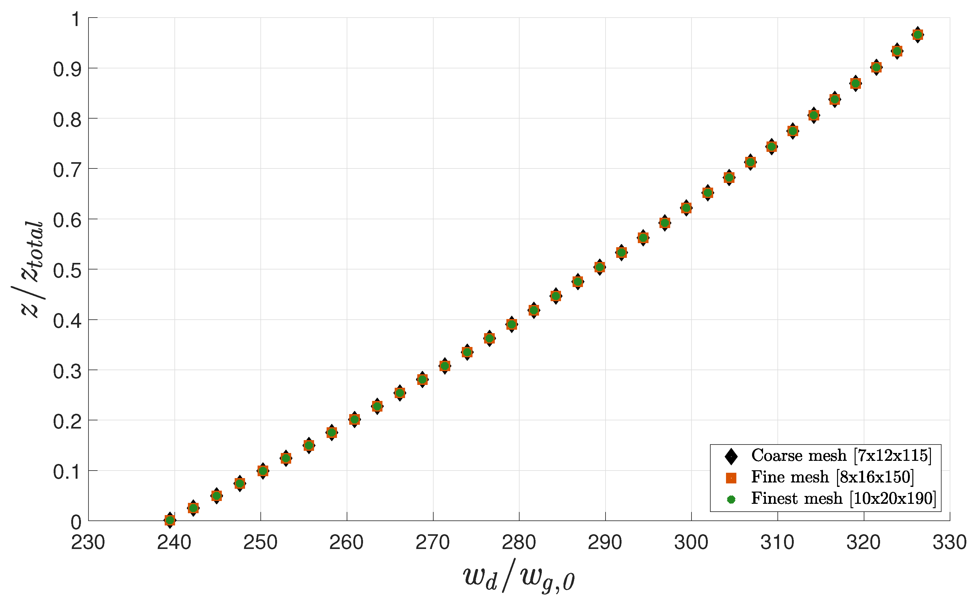
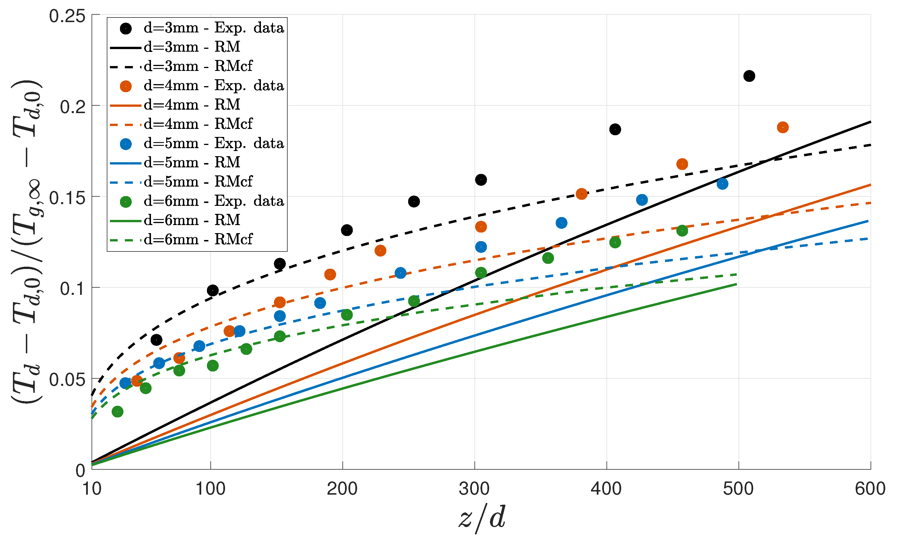
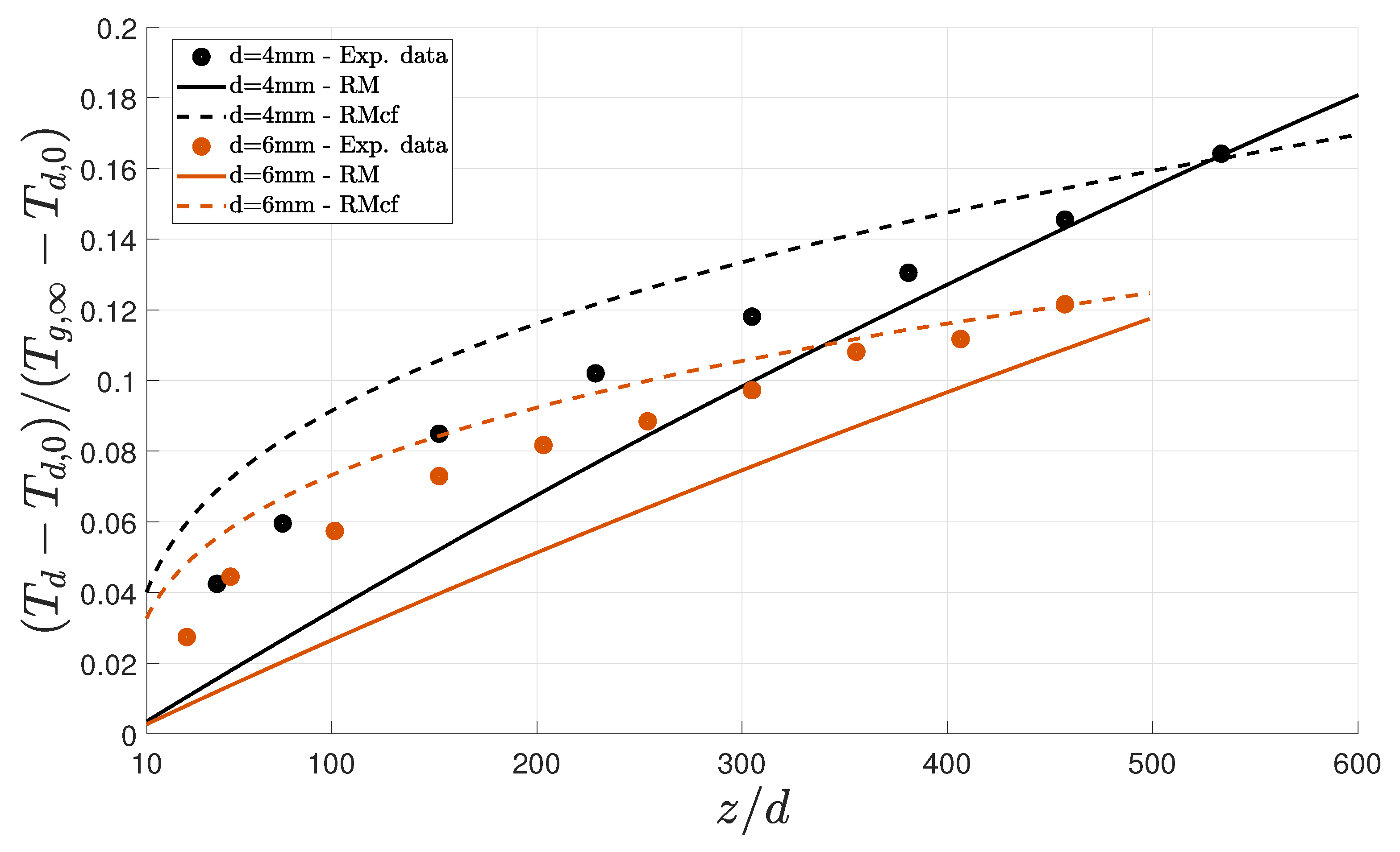
4. Numerical Tests and Validation

To evaluate the cooling rate over time, two distinct parameters were monitored: the droplet temperature, $T_d$, and its falling height, z. These parameters are presented in a non-dimensional way to enable a fair comparison of the phenomenon for different conditions. The droplet non-dimensional falling height was evaluated in relation to its diameter, while a temperature ratio ($\left(T_d-T_{d,0}\right)/\left(T_{g,\infty }-T_{d,0}\right)$) was considered for the cooling process.

However, to ensure that the numerical results were not affected by the solver’s numerics, a grid independence analysis was carried out using three levels of refinement in a structured orthogonal mesh of rectangular elements, with 9660 (coarse mesh), $\mathrm{19,200}$ (fine mesh) and $\mathrm{38,000}$ (finest mesh) points. Figure 2 shows a comparison between these three grids for a droplet diameter of 3 $\mathrm{m}$$\mathrm{m}$ and a relative humidity ratio of $0.29$. The falling height was represented as a function of the vertical velocity component. Since no significant deviation was observed, the fine mesh was used in the computations.

Figure 3 depicts the temperature variation of free-falling water droplets with diameters of 3 and 5 $\mathrm{m}$$\mathrm{m}$ and a humidity ratio of $0.29$. In the figure, the Ranz–Marshall correlations (RM) are compared with the corrected formulations (RMcf) and validated with experimental measurements [44]. Differences between both correlations are evident in the results. While the complete mixing model, corresponding to the Ranz–Marshall correlations, led to an under-prediction of the droplets’ cooling rates, the introduction of vibrations and deformations (RMcf) led to a closer agreement with the experimental data up to a distance of 80 diameters. Moreover, by including the effects of vibrations and deformations, the initial curvature of the temperature profile was retrieved. Nevertheless, as the distance increased, the experimental data behavior and the numerical predictions started to diverge.

Upon increasing the humidity ratio from $0.29$ to $0.36$, the cooling of water droplets with diameters of 3, 4, 5 and 6 $\mathrm{m}$$\mathrm{m}$ was observed (Figure 4). A similar pattern was discovered concerning the previous case. While a linear evolution of the cooling rate was observed, when considering the Ranz–Marshall correlation, the corrected formulation led to a close agreement with the experimental data. Given the results, it is possible to observe that the numerical predictions (RMcf) followed the experimental data for all the considered diameters up to a distance of approximately 200 diameters, after which results started to diverge. Comparing the results for a humidity ratio of $0.29$ in Figure 3 with the ones of Figure 4 for a humidity ratio of $0.36$, it is possible to infer the effect of vibrations and deformations for the prediction of droplet cooling rate.

Figure 5 depicts the results for a humidity ratio of $0.52$ and variable droplet diameters of 4 and 6 $\mathrm{m}$$\mathrm{m}$. A distinct behavior was observed concerning the previous results. Overall, the corrected Ranz–Marshall formulation slightly over-predicted the droplet cooling for small distances. In the case of a 4 $\mathrm{m}$$\mathrm{m}$ diameter, a generally accurate representation of the experimental data was observed, while for the 6 $\mathrm{m}$$\mathrm{m}$ case an accentuated over-prediction was evident up to a falling distance of 100 diameters. Concerning the results obtained with the RM correlation, the predicted linear growth approached the experimental data at around a distance of 400 diameters in the 6 $\mathrm{m}$$\mathrm{m}$ droplet.

Lastly, considering the humidity ratio of $1.00$ and droplet diameters of 3, 4, 5 and 6 $\mathrm{m}$$\mathrm{m}$, an almost linear growth of the experimental cooling rate for all droplet diameters considered is evident in Figure 6. Given the high humidity ratio considered and the numerical results obtained with the Ranz–Marshall corrected correlation (RMcf), it is possible to conclude that the influence of vibrations in the cooling rate under these conditions was meager. However, the linear variation retrieved from the RM correlation led to a linear growth that was sharper than the experimental observation. Nevertheless, a good agreement with the experimental data was evident up to a distance of around 200 diameters for the 3, 4 and 5 $\mathrm{m}$$\mathrm{m}$ droplets. The cooling rate over-prediction in the case of the 6 $\mathrm{m}$$\mathrm{m}$ droplet started at around 100 diameters.

5. Concluding Remarks

In this paper, our computational tool developed in-house for the prediction of the cooling rate of free-falling water droplets was successfully implemented and compared with experimental data. This tool was a RANS-based two-way coupling model using a Eulerian–Lagrangian approach to model each of the considered phases.

The two-way coupling model, which considers the interactions between droplets and the surrounding environment, showed an overall close agreement with experimental data. Furthermore, the consideration of vibrations and deformations through the introduction of an appropriate empirical correlation allowed for the determination of initial curvature of the cooling rate, while the impact of vibrations was found to be meager at high humidity ratios. This suggests the presence of a transition criterion set at intermediate humidity levels that is closely related to increasing droplet diameter.

References

1. Cao, Y.; Wu, Z.; Su, Y.; Xu, Z. Aircraft flight characteristics in icing conditions. Prog. Aerosp. Sci. 2015, 74, 62–80. [Google Scholar] [CrossRef]
2. Cao, Y.; Tan, W.; Wu, Z. Aircraft icing: An ongoing threat to aviation safety. Aerosp. Sci. Technol. 2018, 75, 353–385. [Google Scholar] [CrossRef]
3. Stebbins, S.J.; Loth, E.; Broeren, A.P.; Potapczuk, M. Review of computational methods for aerodynamic analysis of iced lifting surfaces. Prog. Aerosp. Sci. 2019, 111, 100583. [Google Scholar] [CrossRef]
4. Khalil, E.E.; Sobhi, M. CFD Simulation of Thermal and Energy Performance for a Display Cabinet Refrigerator Containing a Phase Change Material (PCM). In Proceedings of the AIAA Propulsion and Energy 2020 Forum, Virtual, 24–28 August 2020. [Google Scholar] [CrossRef]
5. Fakorede, O.; Feger, Z.; Ibrahim, H.; Ilinca, A.; Perron, J.; Masson, C. Ice protection systems for wind turbines in cold climate: Characteristics, comparisons and analysis. Renew. Sustain. Energy Rev. 2016, 65, 662–675. [Google Scholar] [CrossRef]
6. Yancheshme, A.A.; Allahdini, A.; Maghsoudi, K.; Jafari, R.; Momen, G. Potential anti-icing applications of encapsulated phase change material-embedded coatings: A review. J. Energy Storage 2020, 31, 101638. [Google Scholar] [CrossRef]
7. Shirolkar, J.S.; Coimbra, C.F.M.; McQuay, M.Q. Fundamental aspects of modeling turbulent particle dispersion in dilute flows. Prog. Energy Combust. Sci. 1996, 22, 363–399. [Google Scholar] [CrossRef]
8. Gouesbet, G.; Berlemont, A. Eulerian and Lagrangian approaches for predicting the behaviour of discrete particles in turbulent flows. Prog. Energy Combust. Sci. 1999, 25, 133–159. [Google Scholar] [CrossRef]
9. Patankar, N.A.; Joseph, D.D. Modeling and numerical simulation of particulate flows by the Eulerian–Lagrangian approach. Int. J. Multiph. Flow 2001, 27, 1659–1684. [Google Scholar] [CrossRef] [Green Version]
10. Subramaniam, S. Lagrangian–Eulerian methods for multiphase flows. Prog. Energy Combust. Sci. 2013, 39, 215–245. [Google Scholar] [CrossRef] [Green Version]
11. Uranai, S.; Fukudome, K.; Mamori, H.; Fukushima, N.; Yamamoto, M. Numerical simulation of the anti-icing performance of electric heaters for icing on the NACA 0012 airfoil. Aerospace 2020, 7, 123. [Google Scholar] [CrossRef]
12. Messinger, B.L. Equilibrium temperature of an unheated icing surface as a function of air speed. J. Aeronaut. Sci. 1953, 20, 29–42. [Google Scholar] [CrossRef]
13. Peng, K.; Xing, T.; Yi, L.; Yun, Y.H. Effects of turbulent dispersion on water droplet impingement based on statistics method. Int. J. Aeronaut. Space Sci. 2018, 19, 330–339. [Google Scholar] [CrossRef]
14. Fatahian, H.; Salarian, H.; Eshagh Nimvari, M.; Khaleghinia, J. Effect of Gurney flap on flow separation and aerodynamic performance of an airfoil under rain and icing conditions. Acta Mech. Sin. 2020, 36, 659–677. [Google Scholar] [CrossRef]
15. Lian, W.; Zhao, L.; Xuan, Y.; Shen, J. A modified spongy icing model considering the effect of droplets retention on the ice accretion process. Appl. Therm. Eng. 2018, 134, 54–61. [Google Scholar] [CrossRef]
16. Mason, J.; Strapp, W.; Chow, P. The ice particle threat to engines in flight. In Proceedings of the 44th AIAA Aerospace Sciences Meeting and Exhibit, Reno, NV, USA, 9–12 January 2006. [Google Scholar]
17. Bucknell, A.; McGilvray, M.; Gillespie, D.R.H.; Jones, G.; Collier, B. A thermodynamic model for ice crystal accretion in aircraft engines: EMM-C. Int. J. Heat Mass Transf. 2021, 174, 121270. [Google Scholar] [CrossRef]
18. Mason, J.G.; Chow, P.; Fuleki, D.M. Understanding Ice Crystal Accretion and Shedding Phenomenon in Jet Engines Using a Rig Test. J. Eng. Gas Turbines Power 2010, 133, 041201. [Google Scholar] [CrossRef]
19. Al-Khalil, K.M.; Keith, T.G.; De Witt, K.J. Icing calculations on a typical commercial jet engine inlet nacelle. J. Aircr. 1997, 34, 87–93. [Google Scholar] [CrossRef]
20. Zheng, M.; Guo, Z.; Dong, W.; Guo, X. Experimental investigation on ice accretion on a rotating aero-engine spinner with hydrophobic coating. Int. J. Heat Mass Transf. 2019, 136, 404–414. [Google Scholar] [CrossRef]
21. Norde, E.; Senoner, J.M.; van der Weide, E.T.A.; Trontin, P.; Hoeijmakers, H.W.M.; Villedieu, P. Eulerian and Lagrangian ice-crystal trajectory simulations in a generic turbofan compressor. J. Propuls. Power 2019, 35, 26–40. [Google Scholar] [CrossRef]
22. Feng, Z.G.; Michaelides, E.E. The immersed boundary-lattice Boltzmann method for solving fluid–particles interaction problems. J. Comput. Phys. 2004, 195, 602–628. [Google Scholar] [CrossRef]
23. Ireland, P.J.; Desjardins, O. Improving particle drag predictions in Euler–Lagrange simulations with two-way coupling. J. Comput. Phys. 2017, 338, 405–430. [Google Scholar] [CrossRef] [Green Version]
24. Ching, E.J.; Brill, S.R.; Barnhardt, M.; Ihme, M. A two-way coupled Euler-Lagrange method for simulating multiphase flows with discontinuous Galerkin schemes on arbitrary curved elements. J. Comput. Phys. 2020, 405, 109096. [Google Scholar] [CrossRef]
25. Oefelin, J.; Yang, V. High pressure spray field dynamics in turbulent mixing layers. In Proceedings of the 31st Joint Propulsion Conference and Exhibit, AIAA. San Diego, CA, USA, 10–12 July 1995. [Google Scholar] [CrossRef]
26. Gosman, A.D.; loannides, E. Aspects of computer simulation of liquid-fueled combustors. J. Energy 1983, 7, 482–490. [Google Scholar] [CrossRef]
27. Kazemi, S.; Adib, M.; Amani, E. Numerical study of advanced dispersion models in particle-laden swirling flows. Int. J. Multiph. Flow 2018, 101, 167–185. [Google Scholar] [CrossRef]
28. Faeth, G.M. Evaporation and combustion of sprays. Prog. Energy Combust. Sci. 1983, 9, 1–76. [Google Scholar] [CrossRef]
29. Faeth, G.M. Mixing, transport and combustion in sprays. Prog. Energy Combust. Sci. 1987, 13, 293–345. [Google Scholar] [CrossRef] [Green Version]
30. Sommerfeld, M. Analysis of isothermal and evaporating turbulent sprays by phase-Doppler anemometry and numerical calculations. Int. J. Heat Fluid Flow 1998, 19, 173–186. [Google Scholar] [CrossRef]
31. Barata, J. Modelling of biofuel droplets dispersion and evaporation. Renew. Energy 2008, 33, 769–779. [Google Scholar] [CrossRef]
32. Rodrigues, C.; Barata, J.; Silva, A. Modeling of evaporating sprays impinging onto solid surfaces. J. Thermophys. Heat Trans. 2017, 31, 109–119. [Google Scholar] [CrossRef]
33. Launder, B.E.; Spalding, D.B. The numerical computation of turbulent flows. Comput. Methods Appl. Mech. Eng. 1974, 3, 269–289. [Google Scholar] [CrossRef]
34. Crowe, C.T.; Schwarzkopf, J.D.; Sommerfeld, M.; Tsuji, Y. Multiphase Flows with Droplets and Particles, 2nd ed.; CRC Press: Boca Raton, FL, USA, 2011. [Google Scholar] [CrossRef]
35. Hindmarsh, J.P.; Russell, A.B.; Chen, X.D. Experimental and numerical analysis of the temperature transition of a suspended freezing water droplet. Int. J. Heat Mass Transf. 2003, 46, 1199–1213. [Google Scholar] [CrossRef]
36. Strub, M.; Jabbour, O.; Strub, F.; Bédécarrats, J.P. Experimental study and modelling of the crystallization of a water droplet. Int. J. Refrig. 2003, 26, 59–68. [Google Scholar] [CrossRef]
37. Tabakova, S.; Feuillebois, F.; Radev, S. Freezing of a suspended supercooled droplet with a heat transfer mixed condition on its outer surface. AIP Conf. Proc. 2009, 1186, 240–247. [Google Scholar] [CrossRef]
38. Tanner, F.X. Droplet freezing and solidification. In Handbook of Atomization and Sprays: Theory and Applications; Ashgriz, N., Ed.; Springer: Boston, MA, USA, 2011. [Google Scholar] [CrossRef]
39. Akhtar, S.; Xu, M.; Sasmito, A.P. Development and validation of a semi-analytical framework for droplet freezing with heterogeneous nucleation and non-linear interface kinetics. Int. J. Heat Mass Transf. 2020, 166, 120734. [Google Scholar] [CrossRef]
40. Meng, Z.; Zhang, P. Dynamic propagation of ice-water phase front in a supercooled water droplet. Int. J. Heat Mass Transf. 2020, 152, 119468. [Google Scholar] [CrossRef]
41. Myers, T.G.; Hennessy, M.G.; Calvo-Schwarzwälder, M. The Stefan problem with variable thermophysical properties and phase change temperature. Int. J. Heat Mass Transf. 2020, 149, 118975. [Google Scholar] [CrossRef] [Green Version]
42. Ranz, W.E.; Marshall, W.R. Evaporation from drops: Part 1. Chem. Eng. Prog. 1952, 48, 141–146. [Google Scholar]
43. Ranz, W.E.; Marshall, W.R. Evaporation from drops: Part 2. Chem. Eng. Prog. 1952, 48, 173–180. [Google Scholar]
44. Yao, S.C.; Schrock, V.E. Heat and Mass Transfer From Freely Falling Drops. J. Heat Transf. 1976, 98, 120–126. [Google Scholar] [CrossRef]
45. Leonard, B.P. A stable and accurate convective modelling procedure based on quadratic upstream interpolation. Comput. Methods Appl. Mech. Eng. 1979, 19, 59–98. [Google Scholar] [CrossRef]
46. Patankar, S.V.; Spalding, D.B. A calculation procedure for heat, mass and momentum transfer in three-dimensional parabolic flows. Int. J. Heat Mass Transf. 1972, 15, 1787–1806. [Google Scholar] [CrossRef]
47. Lefebvre, A.H.; McDonell, V.G. Atomization and Sprays, 2nd ed.; CRC Press: Boca Raton, FL, USA, 2017. [Google Scholar] [CrossRef]
48. Eckert, E.R.G.; Drake, R.M. Heat and Mass Transfer, 1st ed.; McGraw-Hill Inc.: New York, NY, USA, 1959. [Google Scholar]
49. McQuillan, F.J.; Culham, J.R.; Yovanovich, M.M. Properties of Dry Air at One Atmosphere; Microelectronics Heat Transfer Lab—University of Waterloo: Waterloo, ON, Canada, 1984. [Google Scholar]
50. Lemmon, E.W.; McLinden, M.O.; Friend, D.G. Thermophysical Properties of Fluid Systems in NIST Chemistry WebBook, NIST Standard Reference Database Number 69; Checked on 8th March 2021; National Institute of Standards and Technology: Gaithersburg, MD, USA, 1997; p. 20899. [Google Scholar] [CrossRef]
Figure 1. Description of the computational domain.
Aerospace 08 00270 g001
Figure 2. Grid independence study for three distinct grids.
Aerospace 08 00270 g002
Figure 3. Variation in the temperatures of single water droplets falling through the air, subjected to a humidity ratio of 0.29 .
Aerospace 08 00270 g003
Figure 4. Variation in the temperatures of single water droplets falling through the air, subjected to a humidity ratio of 0.36 .
Aerospace 08 00270 g004
Figure 5. Variation in the temperatures of single water droplets falling through the air, subjected to a humidity ratio of 0.52 .
Aerospace 08 00270 g005
Figure 6. Variation in the temperatures of single water droplets falling through the air, subjected to a humidity ratio of 1.00 .
Aerospace 08 00270 g006