Aircraft Engine Gas-Path Monitoring and Diagnostics Framework Based on a Hybrid Fault Recognition Approach

Abstract

Considering the importance of continually improving the algorithms in aircraft engine diagnostic systems, the present paper proposes and benchmarks a gas-path monitoring and diagnostics framework through the Propulsion Diagnostic Methodology Evaluation Strategy (ProDiMES) software developed by NASA. The algorithm uses fleet-average and individual engine baseline models to compute feature vectors that form a fault classification with healthy and faulty engine classes. Using this classification, a hybrid fault-recognition technique based on regularized extreme learning machines and sparse representation classification was trained and validated to perform both fault detection and fault identification as a common process. The performance of the system was analyzed along with the results of other diagnostic frameworks through four stages of comparison based on different conditions, such as operating regimes, testing data, and metrics (detection, classification, and detection latency). The first three stages were devoted to the independent algorithm development and self-evaluation, while the final stage was related to a blind test case evaluated by NASA. The comparative analysis at all stages shows that the proposed algorithm outperforms all other diagnostic solutions published so far. Considering the advantages and the results obtained, the framework is a promising tool for aircraft engine monitoring and diagnostic systems.

1. Introduction

Over the decades, maintenance programs in gas turbines have evolved from simple to more complex and complete strategies, such as condition-based maintenance (CBM). CBM helps to detect turbomachinery problems, extend machine life, maintain high reliability, reduce operation and maintenance costs, and even avoid catastrophic situations through the use of monitoring and diagnostic systems [1]. This is of vital importance, as evidenced by a previous study [2] showing that in all the causes of commercial flight accidents in the world that occurred from 1990 to 2006, equipment damage was found to be responsible for 23% of the accidents, and of this proportion, 64% of the accidents were related to gas turbine faults. From an economical point of view, the estimated annual fuel costs of the U.S civilian fleet reached 35 billion dollars just some years ago [3].

Due to the increasing safety standards in aviation, condition-monitoring systems need to be continuously improved to correctly detect and identify potential aircraft engine faults, creating demands for research with a focus on improving algorithms and software related to different diagnostic stages. The stages of a diagnostic system are usually data acquisition and processing, monitoring (anomaly detection), diagnostics (fault identification), and prognostics. Each of these stages depends on independent and complex algorithms that require years of work, and their integration into a complete, efficient, and robust system is one of the most important goals of gas turbine engine-health management [4].

Modern gas turbine engines employ different types of condition monitoring techniques, such as vibration analysis, thermography, lubricant analysis, acoustic emission, and gas-path analysis (GPA), and they can be implemented in a separated or integrated way through information-fusion methods [5]. GPA is one of the most common strategies in gas turbine diagnostics. It uses measurements sensed and collected along the air/gas flow path in the gas turbine (temperatures, pressures, rotation speeds, etc.) to constantly monitor, diagnose, and predict the overall engine state without stopping its operation [6,7]. Combined with machine learning and pattern-recognition techniques, the GPA approach can be an efficient tool to diagnose complex and hidden engine faults. Many machine-learning techniques have been employed for gas turbine diagnostics, for example, support vector machines (SVM) [8], genetic algorithms [9], fuzzy logic [10] and neuro-fuzzy inference systems [11], multi-layer perceptron (MLP) [12], probabilistic neural network (PNN) [13], and extreme learning machines (ELM) [14,15].

In any machine-learning method, a trade-off between accuracy and computational complexity must be considered. This means that it is difficult to design a method that is fast while also achieving the best performance. To solve this problem, hybrid approaches have been designed to combine the best characteristics of different methods in an efficient way [16,17,18]. Thus, the limitations of one method can be overcome by the advantages of another.

Despite the advances in the development of different gas turbine fault-recognition techniques, they have been applied to different types of conditions, engines, systems, subsystems, fault scenarios, metrics, etc. This makes it impossible to correctly compare the diagnostic methodologies. To solve this problem, the NASA Glenn Research Center developed a benchmarking platform called ProDiMES (Propulsion Diagnostic Method Evaluation Strategy) that enables specialists to design and evaluate in an objective and fair manner different engine gas-path diagnostic methodologies [19,20,21]. Based on a physics-based thermodynamic model, the tool simulates a fleet of commercial aircraft engines that produce steady-state gas-path measurements registered for every flight for healthy and faulty engines under variable flight conditions. A diagnostic framework analyzes the registered data, producing diagnostic decisions. The effectiveness of the diagnostic system can be measured through different performance metrics. The results published so far about different aircraft engine gas-path monitoring and diagnostic frameworks designed and validated on the ProDiMES software are briefly reviewed below.

Simon et al. [19] evaluated the performance of an example diagnostic solution consisting of three steps related to trend monitoring, anomaly detection, and event isolation. Simon et al. [21] presented four diagnostic approaches: (1) Weighted Least-Squares-based algorithm (WLS) that uses measurement data correction and computes smoothed residuals based on a fleet average engine model for trend monitoring. A backward difference algorithm for computing residual gradients and a threshold are used for anomaly detection. After obtaining anomaly signature vectors, the fault-isolation problem is solved by selecting the fault most likely to be the cause of the observed anomaly. This is achieved through a weighted least-squares estimation method and the application of a fault influence coefficient matrix; (2) PNN-based algorithm that applies the same three steps as in WLS, but a PNN with anomaly signature vectors as inputs is trained instead to isolate faults; (3) Performance Analysis Tool with Kalman Filter (PATKF) is composed by three modules: (a) tracking of progressive degradation with a constant gain-extended Kalman filter that estimates health parameters; (b) an anomaly detection step that sequentially analyzes residuals under the assumptions that an abrupt fault has occurred or not. A comparison between the maximum value of a likelihood ratio over a sliding flight window and a threshold determines the event of the fault or the healthy condition; and (c) a fault-isolation stage that works with a regularized WLS; and (4) Generalized Estimator (GE). It consists of a three-stage procedure with a linear state-space representation of the engine model, a fault detection estimator based on the comparison of filtered residual components and a predefined threshold for detecting the presence of a fault, and a fault-isolation estimator based on adaptive estimation techniques.

Jaw et al. [8] compared seven machine learning methods in three stages for binary and multi-class problems: (1) Naïve Bayes (NB) that estimates the probability of each fault class given a test sample, (2) Decision Tree (DT) that chooses a class by making a sequence of decisions organized as a tree, (3) K-Nearest Neighbors (KNN) that selects a class through the majority vote of the k-nearest training elements of a test sample, (4) Linear Support Vector Machine (LSVM) that finds a hyperplane with maximal margin to better classify samples, (5) nonlinear SVM (NSVM) that maps the space of input vectors into a higher-dimensional space to perform class separation, (6) a hierarchical linear SVM with kernel sliced inverse regression (kSIR) called HSVMkSIR that reduces the dimensionality of the data to train multiple classifiers and hierarchically identify faults, and (7) a non-linear SVM with kSIR version called NSVMkSIR.

Borguet et al. [22] developed a regression-based approach for modeling a fleet of jet engines from historical operational data considering engine-to-engine variations. The models are assessed quantitatively with coefficient determination and then applied to the ProDiMES turbofan engine fleet to perform anomaly detection. Using different diagnosis analysis and validation data, Loboda et al. [23] benchmarked a data-driven gas turbine diagnostic methodology based on three well-known methods: (1) multi-layer perceptron, (MLP) whose learning process consists of looking for such weight and bias coefficients that minimize the error through the backpropagation algorithm. The output is a measure of the closeness of an input sample and a class. In the decision stage, the class that has the maximum output is selected; (2) probabilistic neural network (PNN), whose hidden neurons based on radial basis functions produce responses that indicate how close an input vector is to the training samples. These hidden neurons are connected to only one output neuron. The output neuron receives a sum (a probability of the class) of the responses related to the training vectors of the corresponding class and a competitive transfer function chooses the class that produces the maximum probability; and (3) a nonlinear SVM.

Koskoletos et al. [13] proposed a diagnostic framework that integrated the stages of data processing, fault detection based on a cumulative sum algorithm, and fault identification intended to evaluate six different gas-path methods: PNN, KNN, estimation of health parameters with an optimization algorithm, a combinatorial approach through the examination of all possible combinations of health parameters and measurements, a method based on an adaptive engine model, and a hybrid method using PNN and adaptive model. This last hybrid approach uses an adaptive engine model and the a-priori information about the occurrence of a component fault in the engine. It is applied only when the PNN outputs a component fault as the most probable to happen and the adaptive method produces the final classification. For actuator and sensor faults, PNN performs the classification. The methods are tested in three stages considering a simplified scenario with module faults; a more complex scenario with module, actuator, and sensor faults; and the blind test case.

Calderano et al. [24] implemented and evaluated an enhanced diagnostic method based on upper and lower singleton type-2 fuzzy logic system (ULST2-FLS) that works with a pre-processing module as proposed in [6,21], including parameter correction, residual computation for trend monitoring, backward differences, and normalization; and anomaly detection and classification modules that use ULST2-FLS. The classification method first receives crisp inputs that pass through a fuzzifier block, producing fuzzy sets. Applying rules in an inference engine, the fuzzy output sets feed an output processing block formed by a type-reducer set and a defuzzifier that finally returns crisp outputs. Teixeira et al. [25] proposed the Wang–Mendel Fuzzy Logic System (WMFLS), which has a similar procedure to ULST2-FLS, with the main difference that the former employs a type-1 fuzzy logic system that automatically extracts rules via the Wang–Mendel method.

Considering the advantages of ProDiMES, the main objective of the present paper is to continue the improvement of algorithms by proposing an aircraft engine monitoring and diagnostic hybrid approach. The results of the proposed system are compared with all the aforementioned diagnostic algorithms. The main contributions of this paper are:

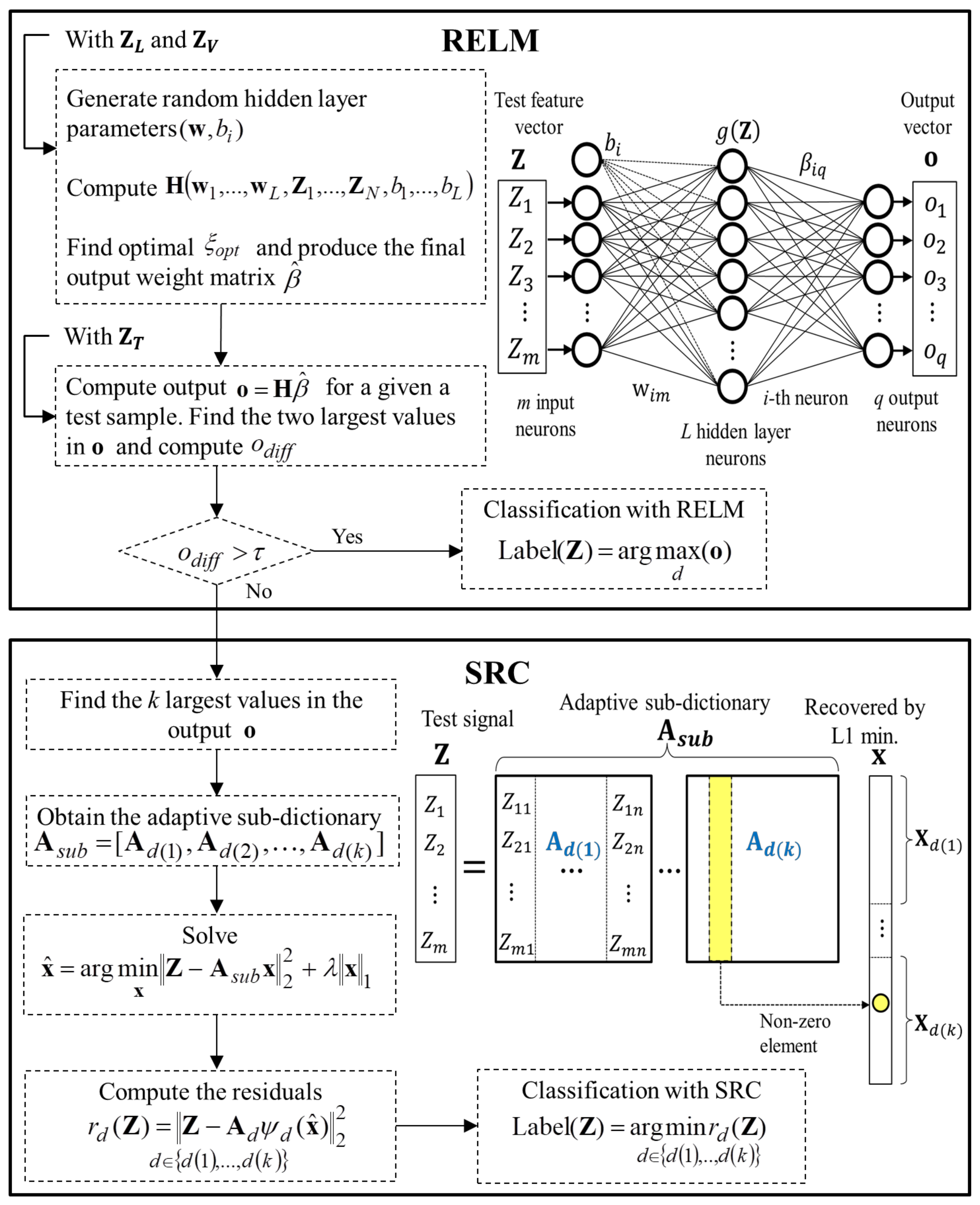
• We propose a diagnostic system based on a hybrid fault-recognition method that exploits the advantages of the low computational complexity of ELM and high recognition accuracy and noise-robustness of sparse representation classification method to improve the aircraft engine diagnostic decisions.
• Up to now, the majority of the published solutions using ProDiMES work with an anomaly detection algorithm followed by another fault identification algorithm, causing delays in the diagnostic decisions. The present methodology performs both stages as a common process by computing their corresponding performance metrics at the same time and with the same fault recognition algorithm.
• The paper contributes to the advancement of the state-of-the-art in the area of gas turbine engine health management since it provides a robust and fair comparison with all the available diagnostic algorithms published in the literature using ProDiMES from worldwide leading and established researchers, including the authors of the benchmarking platform. Additionally, the work stimulates the competition between diagnostic solutions and further development of the area of gas turbine diagnostics.

The work is organized as follows. Section 2 gives the general benchmarking process in ProDiMES. Section 3 introduces the proposed diagnostic framework. Section 4 presents the results of the comparison with other diagnostic approaches. The Discussion section (Section 5) addresses the major findings of the paper.

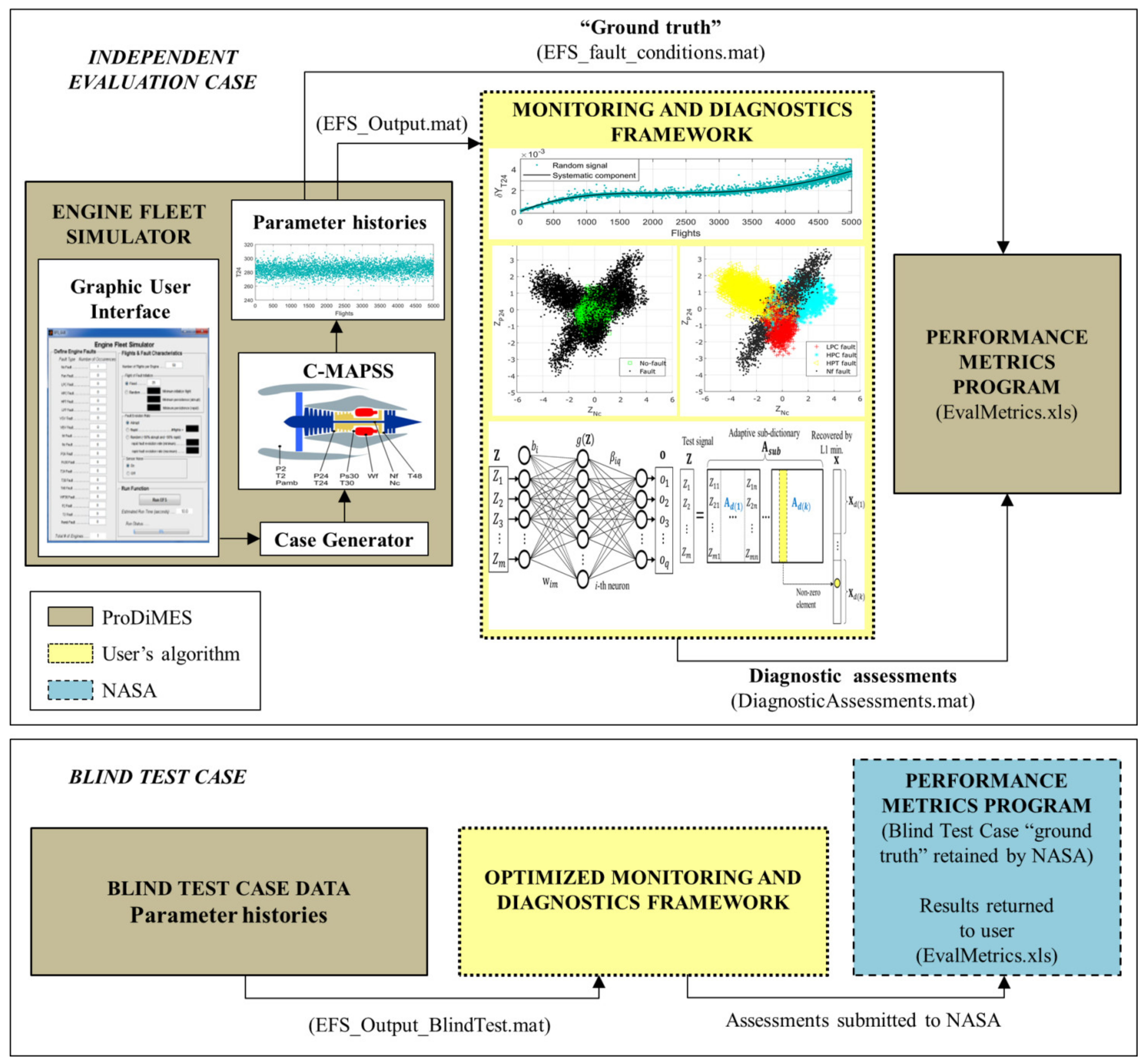
2. ProDiMES Benchmarking Process

In this section, an overview of ProDiMES and its benchmarking process is given. Appendix A contains additional information about the engine layout and diagnostic performance metrics. A more detailed description of the software design and operation can be found in the official ProDiMES user’s guide [20] and NASA’s software catalog available at https://software.nasa.gov (accessed on 15 August 2021).

The process of aircraft engine fleet performance assessment through ProDiMES has two functionalities: (1) an independent evaluation case that assists in the development of diagnostic algorithms and self-assessment through the generation of engine data by the user, the knowledge of true fault/no-fault conditions (a.k.a. “ground-truth” information), and the computation of diagnostic performance metrics and (2) a blind test case intended to perform a fair comparison between different optimized diagnostic methodologies from other researchers employing a unique dataset (available in a ProDiMES folder) generated by NASA, who withholds the blind test case “ground-truth” information. NASA receives and evaluates the diagnostic assessments, returning the metrics along with the anonymous results of other participants. Figure 1 illustrates these two functionalities with their corresponding blocks and output information (mat-files or Excel spreadsheets) produced by the ProDiMES platform, by the user’s diagnostic algorithm, or by NASA.

2.1. Engine Fleet Simulator

The platform core is the Engine Fleet Simulator (EFS) that works with the steady-state version of the Commercial Modular Aero-Propulsion System Simulation (C-MAPSS) [26], a software that provides a realistic simulation of a large, commercial two-spool turbofan engine (See Appendix A). In a first step, the participants must set in a graphic user interface (GUI) all the required simulation characteristics that include the fault scenario, number of occurrences per scenario, the number of flights over which the sensed parameter history will be collected in an engine (with a maximum of 5000 flight cycles), the fault evolution rate (abrupt, rapid, or random), flight of fault initiation (fixed or random) with a minimum persistence for abrupt and rapids faults, and sensor noise selector (on or off). ProDiMES works with small, medium, and large faults. In addition, an average of all three faults is considered.

After defining the values in the GUI, the Case Generator randomly assigns to each engine in the fleet realistic and unique operating condition attributes and degradation profiles. This includes power settings at take-off and cruise regimes, the cities where the aircraft takes off and lands, ambient conditions, Mach number, etc. The software emulates long-term engine performance deterioration as a natural part of engine service life due to fouling, erosion, and other abrasive conditions in five major components: fan, low-pressure compressor (LPC), high-pressure compressor (HPC), high-pressure turbine (HPT), and low-pressure turbine (LPT). Efficiency η and flow capacity γ are the two health parameters in each component that modify the normal engine behavior. However, ProDiMES also considers short-term degradation in the form of rapid or abrupt faults since they evolve in a much faster timescale than long-term degradation. Apart from the no-fault case,

Table 1. Simulated faults in ProDiMES [20].

ID	Fault Type	Fault Description	Fault Magnitude
0	None	No-fault	None
1	Component	Fan	1 to 7%
2		LPC	1 to 7%
3		HPC	1 to 7%
4		HPT	1 to 7%
5		LPT	1 to 7%
6	Actuator	VSV	1 to 7%
7		VBV	1 to 19%
8	Sensor	Nf	±1 to 10 σ
9		Nc	±1 to 10 σ
10		P24	±1 to 10 σ
11		Ps30	±1 to 10 σ
12		T24	±1 to 10 σ
13		T30	±1 to 10 σ
14		T48	±1 to 10 σ
15		Wf	±1 to 10 σ
16		P2	±1 to 10 σ
17		T2	±1 to 10 σ
18		Pamb	±1 to 19 σ

presents 18 fault scenarios with uniformly distributed magnitudes related to component, actuator, and sensor faults (in units of standard deviation from measurement noise). C-MAPSS finally receives the Case Generator outputs and produces sensed parameter histories for each engine in the fleet.

Table 2. Operating conditions U in ProDiMES [20].

ID	Symbol	Description	Units
1	Nf	Physical fan speed	rpm
2	P2	Total pressure at fan inlet	psia
3	T2	Total temperature at fan inlet	°R
4	Pamb	Ambient pressure	psia

contains four operating conditions U (ambient and control variables) and

Table 3. Gas-path monitored variables Y in ProDiMES [20].

ID	Symbol	Description	Units
1	Nc	Physical core speed	rpm
2	P24	Total pressure at LPC outlet	psia
3	Ps30	Static pressure at HPC outlet	psia
4	T24	Total temperature at LPC outlet	°R
5	T30	Total temperature at HPC outlet	°R
6	T48	Total temperature at HPT outlet	°R
7	Wf	Fuel flow	pps

shows seven gas-path monitored variables Y corresponding to a standard measurement system. Thus, this raw simulated information is ready to be processed and interpreted by a diagnostic framework.

2.2. Performance Metrics

The performance estimation program is a routine contained in ProDiMES that receives diagnostic assessments and then evaluates the detection and classification capabilities of candidate diagnostic methods. To compute the metrics, it is necessary to compare the diagnostic assessments and the ground-truth information. The ProDiMES performance metrics are grouped in three categories [20]:

• Detection: true-positive rate (TPR), true-negative rate (TNR), false negative rate (FNR), and false positive rate (FPR).
• Classification: correct classification rate (CCR), misclassification rate (MCR), and kappa coefficient (it indicates the capability of the diagnostic framework to accurately classify a fault considering the expected number of correct classifications that occur by chance. If kappa = 1, then the diagnostic technique produces a perfect classification; if kappa < 0, then the classification is worse than expected).
• Latency metrics: detection latency as the average number of flights a fault persists before a true-positive detection and classification latency as the average number of flights a fault must persist prior to correct classification.

In the present paper, an extra metric $\overline{P}$ is employed to analyze the global diagnostic accuracy of the recognition method, allowing the adjustment of the algorithm according to the requirements in each comparison stage. This metric is computed as a weighted mean probability of the main diagonal elements of a confusion matrix considering the number of samples in each class for healthy and faulty cases.

3. Proposed Monitoring and Diagnostics Framework

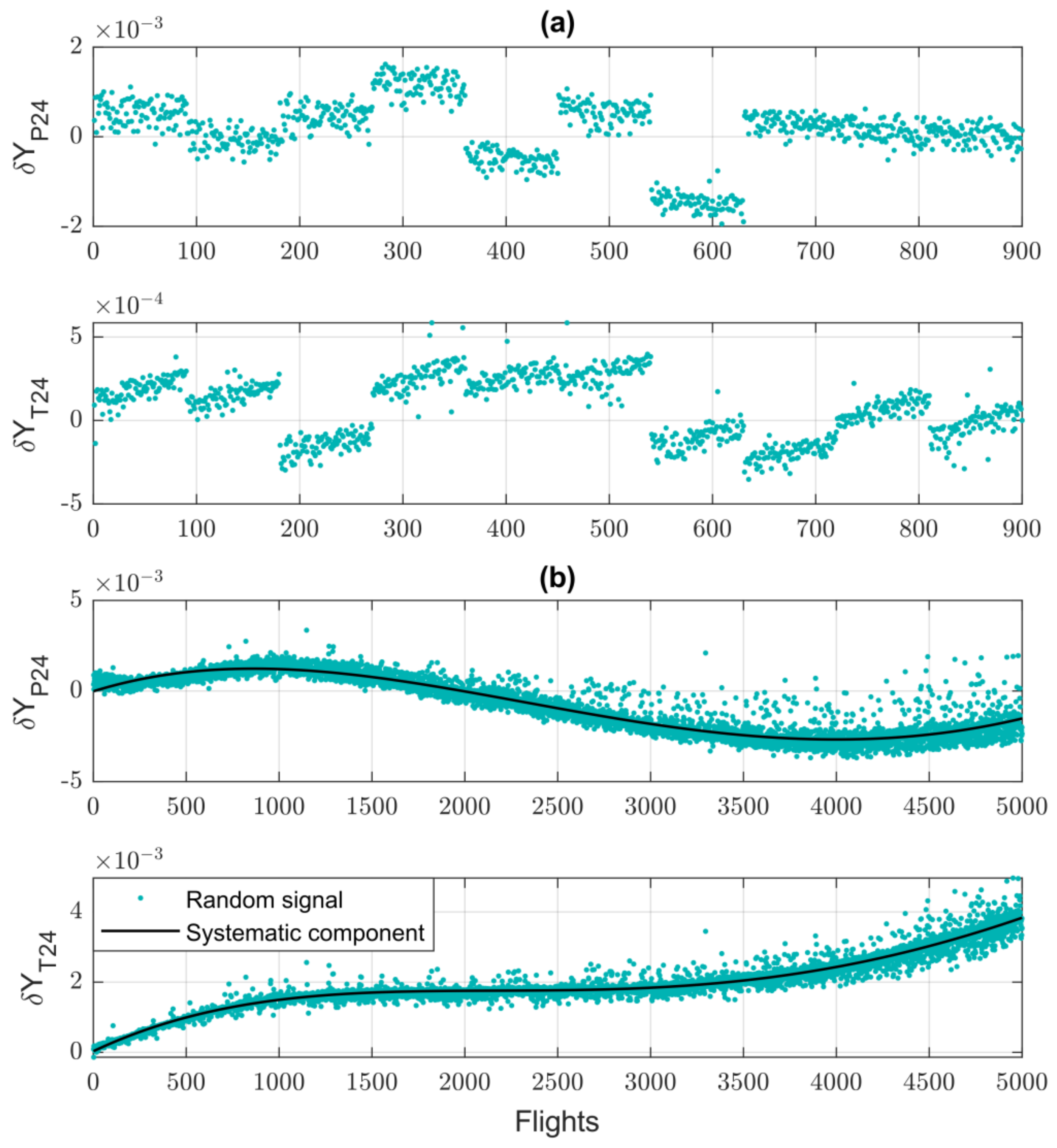
3.1. Averaged Baseline Model for Engine Fleet

It is common that in a gas turbine diagnostic process, engine health diagnostic indicators are computed. One typical indicator is a deviation, which contains information about the current engine state and reveals engine degradation trending and changes due to faults. Deviations can be calculated as relative differences between actual measurements and healthy engine values [22]. Considering a gas-path monitored variable Y, a deviation is expressed as:

$$\delta Y^{*}=\frac{Y^{*}-Y_0\left(U\right)}{Y_0\left(U\right)}$$

(1)

where Y* is an actual measured value and $Y_0\left(U\right)$ is the normal engine value (also called baseline function) depending on operating conditions. Second-order polynomials are good estimators of healthy engine performance at steady-state and transients [27]. For one monitored variable Y and four operating conditions U, such a polynomial has the following structure:

$$\begin{array}{l}{Y}_0(U)=c_1+c_{2}Nf+c_3{P}_2+c_{4}T2+c_5{P}_{amb}+c_{6}NfP2+c_{7}NfT2+c_{8}Nf{P}_{amb}+\\ +c_{9}P2T2+c_{10}P2P_{amb}+c_{11}T2P_{amb}+c_{12}N{f}^2+c_{13}P{2}^2+c_{14}T{2}^2+c_{15}{P}_{amb}^2\end{array}$$

(2)

If all measured variables and n flights are considered, Equation (2) can be described in the form of a linear system $Y_0=VC$ and unknown coefficients ${\widehat{c}}_{ij}$, which are contained in a $\left(k\times m\right)$-matrix, are estimated through the least-squares method (LSM):

$$\hat{C}={\left(V^{T}V\right)}^{-1}{V}^T{Y}_0$$

(3)

where $Y_0$ is a $\left(n\times m\right)$-matrix of m measured variables, and $V$ is a $\left(n\times k\right)$-matrix with k elements $\left(1,Nf,P_2,\dots ,T{2}^2,P_{amb}^2\right)$ from operating conditions.

Anomaly detection and fault identification stages highly depend on the quality of deviations, which in turn depend on baseline model adequacy. To achieve this, two steps are proposed: (1) baseline model creation with a proper reference sample and (2) model verification with a test dataset. In the case of the first step, it is important to have a representative engine-fleet dataset with a considerable amount of flights that present a low level of degradation to avoid elevated deviation errors. A reference sample of 100 engines and initial 90 flights per engine is sufficient to obtain an adequate average baseline model [28]. To see the quality of deviations based on this dataset, a sample without noise is generated through ProDiMES using the no-fault case scenario. Figure 2a shows deviations obtained for two gas-path measured variables (total pressure and temperature at LPC outlet) and 900 flights (from 10 engines). For each engine, the low and progressive degradation (pressure drop and temperature increase) in the first 90 flights and the small random flight-to-flight variations are visible. The unique, randomly assigned operating conditions and deterioration profiles for each engine are evident through these deviations.

In the case of the second step, the deviation analysis of individual engines can be employed to verify the effectiveness of the baseline model through the engine lifetime. Figure 2b shows the deviations computed for one engine and all its 5000 successive flights and the same two monitored variables as in Figure 2a. A 4th order polynomial is employed to approximate the systematic component of the signal (general change without noise) and see more clearly the degradation trending. Deviations errors (or noise) can be computed as a difference between the random signal and the systematic component. From the picture, one can observe that the model effectively captures the progressive engine deterioration. Deviation errors are small at the initial flights and increase at the final of the engine lifetime. This is explained by the fact that the influence of operating conditions on the gas-path monitored variables of a degraded engine greatly differs from the baseline model producing an increasingly less accurate model. This should be considered when diagnosing an aged engine to not confuse normal deterioration with faults. It is important to mention that this work considers measurement noise for baseline model creation as a requirement by ProDiMES to develop noise-robust diagnostic systems.

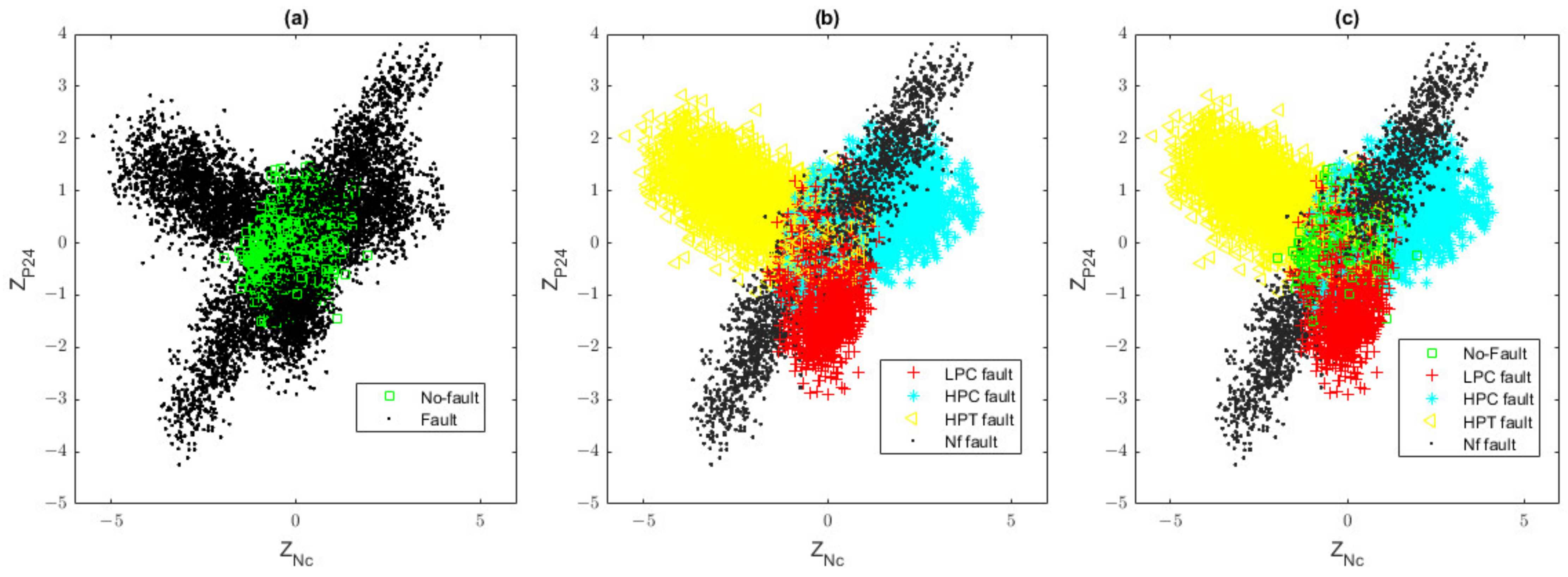
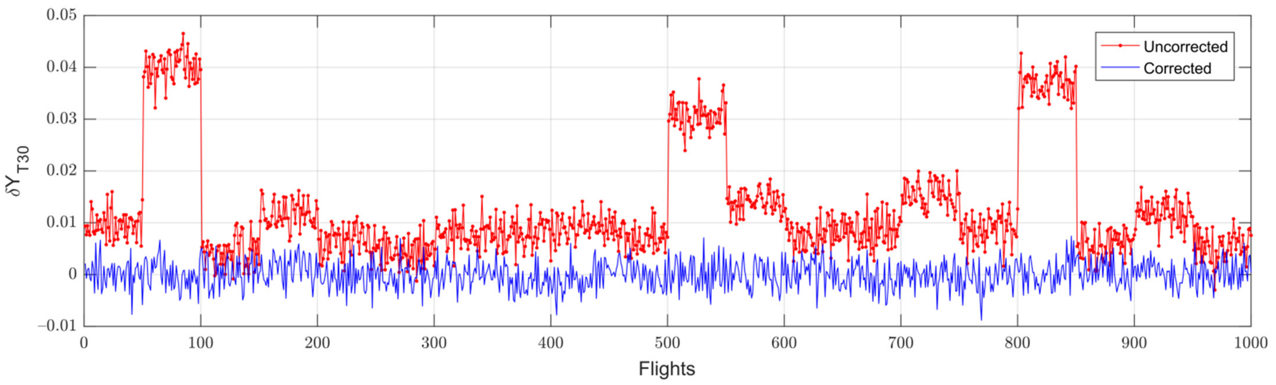
3.2. Baseline Model Correction and Class Formation

Once the baseline model is determined, deviations between healthy and faulty values can be computed. However, it is necessary to correct the deviations through the computation of individual engine baseline models. The reason is that the simulated engines have individual characteristics, such as particular performances and levels of degradation. Since a fleet-average baseline model is employed, the deviations are affected, producing errors for not considering engine individualities. To solve this problem, a correction is made as follows. First, the first ten flights free of any fault in each engine are utilized to compute an average correction coefficient:

$$K_i=\frac{1}{10}{\displaystyle \sum _{j=1}^{10}\delta Y^{*}}$$

(4)

This coefficient is defined as a relative difference between the individual baseline model $Y{I}_{0i}$ and the fleet-average baseline model $Y_0\left(U\right)$. Thus, an individual baseline value is given by:

$$Y{I}_{0i}=Y_{0i}(1+K_i)$$

(5)

Final deviations consider engine individualities and are normalized using a mean deviation error ${\sigma }_{\delta Yi}$ to have a homogeneous diagnostic space:

$$Z_i^{*}=\frac{Y_i^{*}-Y{I}_{0i}}{{\sigma }_{\delta Yi}Y{I}_{0i}}$$

(6)

Figure 3 shows uncorrected deviations applying an average-fleet baseline model (Equation (1)) and corrected deviations based on individual baseline models (Equation (6) without normalization) plotted for one monitored variable and 50 flights from each of 20 different healthy engines (1000 concatenated flights). Since no fault is implanted in the engines, deviations to be employed for monitoring and diagnostics should remain around zero with no significant shifts (except for random noise). Uncorrected deviations do not meet this requirement since they present for each engine abrupt changes and perturbations that can be confused with particular faults. It is clear that computing deviations as a difference between measured values of a particular engine and a generalized fleet-average baseline model (that does not match the specific performance characteristics of such a particular engine) results in a wrong approach that will cause elevated diagnostic errors in further stages. Corrected deviations solve this problem with individual baseline models that correctly reflect the performance of a healthy engine.

Deviations from Equation (6) are filtered for further analysis using exponential moving average (EMA) as follows:

$$Z_{EM{A}_{i,j}}=\alpha Z_{i,j}+\left(1-\alpha \right)Z_{EM{A}_{i,j-1}}$$

(7)

where $\alpha$ is the smoothing factor with values between 0 and 1, and j is the current flight in the engine. In this manner, deviations computed for all monitored variables constitute a feature vector $Z$. Feature vectors form a fault classification with healthy and faulty classes to be recognized by a machine-learning technique in a multidimensional diagnostic space. To that end, measurements from many engines and flights are simulated through ProDiMES and transformed into feature vectors to have a representative no-fault class as well as 18 fault classes. These 19 fault classes with all their corresponding samples form a complete fault classification that is randomly partitioned into two sets: one called learning set $Z_L$ (80–90% of the data) for training the fault recognition technique and another one called validation set $Z_V$ (10–20% of the data) to verify the performance of the trained models for unseen data using k-fold cross-validation. In this process, hyperparameters are also optimized to produce the best recognition performance. Thus, the best-trained model is applied to a third set called testing set $Z_T$. In the present work, this set varies depending on the comparison stage, and it is intended to compare the techniques.

3.3. Hybrid Fault Classification Approach

The hybrid fault classification procedure consists of two parts: the regularized extreme learning machine (RELM) and the sparse representation classification (SRC) block. Figure 4 summarizes the steps in each block.

Block 1: ELM was originally developed as a generalized feed-forward neural network with one hidden layer. Due to its extended use in different applications, there are many network configurations with improved features. ELM differs from many popular ANNs, such as multilayer perceptron, in the following aspects: the hidden node parameters are randomly selected, and only the output parameters are computed; the backpropagation algorithm is replaced by a matrix inverse that is computed only once; and there is no need of network learning iterations for gradient descent. As a result, the training process is less complex and faster.

Considering a training dataset ${\left\{\left(Z_j,t_j\right)\right\}}_{j=1}^N$, where $N$ is the total number of training samples, $Z_j={[Z_{j1,}{Z}_{j2,},\dots ,Z_{jm}]}^T$ is an m-dimensional input feature vector, and $t_j={[t_{j1,}{t}_{j2,},\dots ,t_{jq}]}^T$ is a q-dimensional target vector with values −1 and 1 indicating the category ($d=1\dots q$ classes) each vector belongs to, the ELM structure can be expressed as follows:

$$o_j=f(Z_j)={\displaystyle \sum _{i=1}^{L}g(w_i{}^T{Z}_j+b_i){\beta }_i,\hspace{1em}j=}1,2,\dots ,N$$

(8)

where $o_j$ is the network output or prediction, $g(Z_j)$ is the activation function, $w_i={[w_{i1,}{w}_{i2,},\dots ,w_{im}]}^T$ are the randomly generated weights of the i-th hidden node connected to the input neurons, $b_i$ is the bias, and ${\beta }_i={[{\beta }_{i1,}{\beta }_{i2,},\dots ,{\beta }_{iq}]}^T$ are the output layer weights connected to the hidden neurons.

Since ELM tries to learn pre-defined classes by finding such output layer parameters that minimize the difference between outputs and targets, the problem to solve is presented as:

$$\arg \underset{\beta }{\min }{‖H\beta -T‖}_F$$

(9)

where $\beta ={\left[{\beta }_1,\dots ,{\beta }_L\right]}^T$ is the (q × L) output weight matrix, $T={\left[t_1^T,\dots ,t_N^T\right]}^T$ is the (q × N) target matrix, and $H$ is the hidden layer output matrix for L hidden layer neurons.

$$H=\left[\begin{array}{ccc}g(w_1{}^T{Z}_1+b_1)& \cdots & g(w_L{}^T{Z}_1+b_L)\\ ⋮& \ddots & ⋮\\ g(w_1{}^T{Z}_N+b_1)& \cdots & g(w_L{}^T{Z}_N+b_L)\end{array}\right]$$

(10)

Output weights can be obtained by LSM in the form of $\widehat{\beta }=H$^†$\mathbf{T}$. However, due to the instability problems in the computation of the Moore–Penrose matrix inverse $H$^†, a regularized LSM is employed instead:

$$\arg \underset{\beta }{\min }{‖H\beta -T‖}_F+\frac{1}{\xi }{‖\beta ‖}_F$$

(11)

where $\xi$ is a parameter that balances training error and regularization terms. The leave-one-out cross-validation approach can be used for model selection to search the optimal ${\xi }_{opt}$ that produces the best separating hyperplane [29]. The solution of Equation (11) is:

$$\widehat{\beta }={\left(H^{T}H+{\xi }_{opt}I\right)}^{-1}{H}^{T}T\mathrm{if}L<N\mathrm{or}$$

$$\widehat{\beta }=H^T{\left({\mathrm{HH}}^T+{\xi }_{opt}I\right)}^{-1}T\mathrm{if}L\ge N$$

(12)

where $I$ is the identity matrix. After determining $\hat{\beta }$, the output can be computed as $o=H\widehat{\beta }$, and the label of the class is finally assigned with:

$$\mathrm{Label}(Z)=\arg \underset{d}{\max }(o)$$

(13)

To evaluate different network models, 10-fold cross-validation is performed. At each iteration, new subsets $Z_L$ and $Z_V$ are randomly created from a pre-built fault classification. First, all the N samples of the training data are used to compute the output weights. Then, all the validation samples are introduced by turn to the network to obtain predictions that will serve to form a confusion matrix and compute the diagnostic accuracy $\overline{P}$ of the current model for unseen data. An averaged value of $\overline{P}$ considering all iterations gives the final network classification performance.

After the training-validation process is finished, and a testing feature vector from set $Z_T$ is introduced to the network to generate an output vector $o$, a difference $o_{diff}$ between the two largest values contained in $o$ is computed. Since the RELM classification decision is based on the maximum value in the output, $\mathrm{Label}(Z)=\arg \underset{d}{\max }(o)$, a measure of closeness between the first and second value can reflect, to some extent, how well the RELM decision hyperplane works. If $o_{diff}$ is small, then the network will be prone to misclassification. For that reason, such difference can be employed as a decision rule to separate those samples with high noise levels (resulting in small output differences and erroneous classification) and classify them again but with a more noise-robust method. In this way, for the proposed procedure, if $o_{diff}$ value exceeds a pre-defined threshold $\tau$, then the sample is classified with RELM; otherwise, it is treated as a potential misclassification and reclassified with SCR in the next block.

Block 2: Given a test sample $Z$ as a column vector, the objective of SRC is to reconstruct such original test signal as sparse and exact as possible with a linear combination of training signals from the same class predominantly. This is achieved by obtaining non-zero scalar coefficients $x$ in the location of the corresponding class.

In a classic SRC, an over-complete dictionary approach considers all the training classes to reconstruct the testing signal. However, this approach forms a unique and fixed dictionary that considers unnecessary and uncorrelated classes affecting optimal sparse representation and classification [30]. Besides, testing time increases with the number of classes considered for dictionary formation. To solve these problems, the formation of sub-dictionaries, which contain only the information of similar classes to the testing sample, is considered [31]. The idea is to take into account the indices of the k largest values in the RELM output vector that reflect the most correlated classes and discard those with small values that affect signal reconstruction. Thus, each time a testing sample is classified with SRC, the training atoms (feature vectors) from the same classes of the k largest output values are selected to construct a new sub-dictionary with the structure $A_{sub}=[A_{d(1)},A_{d(2)},\dots ,A_{d(k)}]$, where $d(i)\in \left(1,2,\dots ,q\right)$ is one of the indices of the k largest elements, and $A_{d(i)}$ contains all the training samples from the $d(i)$-th class. The sparse representation coefficients are estimated by solving:

$$\widehat{x}=\arg \underset{x}{\min }{‖Z-A_{sub}x‖}_2^2+\lambda {‖x‖}_1$$

(14)

where $\lambda$ is a scalar parameter that controls the trade-off between sparsity and signal reconstruction. A test sample $Z$ can be classified by the atoms from the class d that produce the minimum residual or reconstruction error (difference between original and reconstructed signal), $r_d(Z)={‖Z-A_d{\psi }_d(\widehat{x})‖}_2^2$, where ${\psi }_d(\hat{x})$ is the characteristic function that only selects the coefficients in vector $\hat{x}$ associated to the class $d\in \left\{d(1),\dots ,d(k)\right\}$. Thus, the classification is given by the expression:

$$\mathrm{Label}(Z)=\underset{d}{\arg \min }{r}_d(Z)$$

(15)

To minimize classification errors and obtain the best classification results in the hybrid approach, it is necessary to search by trial-and-error the optimal values of other important parameters, such as the number of hidden neurons L in RELM, the threshold $\tau$, and the value of k in the adaptive sub-dictionary formation. This can be achieved by varying one parameter by turn and fixing the rest. The configuration of those parameters that produce the highest diagnostic accuracy is then selected.

3.4. Anomaly Detection and Fault Identification as a Common Process

Commonly, in aircraft engine diagnostic systems, anomaly detection is carried out first to know if a potential problem is occurring in the engine. However, many of the faults are difficult to detect due to their small magnitude and high measurement noise, causing them to be confused with healthy states. A noise-robust detection algorithm will try to monitor the progression of such faults considering these negative circumstances. Typically, if an engine health indicator has significantly surpassed an established threshold, then the algorithm confirms the detection of an anomaly. After that, a fault identification procedure is applied to locate and determine the nature of such a fault. All the above-mentioned procedure causes delays in diagnostic decisions, especially if a fault is not detected on time.

The present work proposes a different scheme, with the stages of anomaly detection and fault identification viewed as a recognition problem in a common process. Figure 5 gives an illustration of this concept with feature vectors in the diagnostic space Z for two monitored variables. First, Figure 5a shows a separate example of anomaly detection, where feature vectors only belong to the no-fault class or the fault class. Thus, this stage can be seen as a binary recognition problem by training a classifier with the two classes. After an anomaly is detected, the fault identification stage is performed as a multi-class problem, as shown in Figure 5b. Here, all the samples of different q fault classes are used to train a second classifier and identify new samples. Such consecutive procedure is not convenient since the training and adjustment of two different classifiers may require a significant amount of time, causing delays in making decisions. Instead, as depicted in Figure 5c, a single classifier trained with the samples from the no-fault case and all the fault classes can detect and identify a fault at once. To compute the anomaly detection and fault identification metrics, the same confusion matrix of size [(q + 1) × (q +1)] is employed to extract the corresponding information for each task.

4. Comparison of Diagnostic Frameworks

This stage compares the different diagnostic frameworks benchmarked so far through ProDiMES and reviewed in the Introduction section (Section 1). The comparison analysis is divided into four stages that differ by comparison conditions and are performed one after another. The first three are intended to adjust the proposed algorithm and are related to the Independent Evaluation Case functionality, while the last stage deals with the Blind Test Case, which is the final goal in ProDiMES.

Table 4. Conditions and stages of comparison.

Comparison Conditions	Comparison Options	Comparison Stages
		1	2	3	4
Operating points	Cruise	X	X
	Multipoint			X	X
Diagnostic metrics	$\overline{P}$	X
	ProDiMES metrics	X	X	X	X
Testing Data	Generated by authors		X
	ProDiMES dataset	X	X	X
	Blind test dataset				X

summarizes the comparison conditions that include engine operating points, diagnostic performance metrics employed as criteria, and type of testing data. A diagnostic technique may employ only the cruise data or the data collected at both regimes (cruise and takeoff) a.k.a. multipoint diagnosis. The two options of criteria are the diagnostic accuracy $\overline{P}$ and the diagnostic metrics computed by ProDiMES. Three options of testing data include the sets generated by users, the dataset given in ProDiMES as an example, and ProDiMES blind test dataset. The table indicates the options used at each of the four stages.

4.1. Stage 1: Comparison with Other Diagnostic Frameworks Using ProDiMES Cruise Dataset

The first stage addresses a comparison between the proposed algorithm based on RELM-SRC (and a version of RELM) and three state-of-the-art machine-learning methods benchmarked by Loboda et al. [23]: PNN, MLP, and non-linear SVM. The methods are analyzed under the same conditions and with tuned hyperparameters for a fair comparison. Three training configurations were generated through ProDiMES for the cruise regime to analyze the influence of training dataset size and deviation smoothing with EMA on the diagnostic accuracy $\overline{P}$.

ProDiMES includes an example solution folder with an output file that serves as a test dataset for comparing other diagnostic solutions. The characteristics of this set are presented in

Table 5. Training and testing datasets specifications (Stage 1).

Description	Training Conf.1	Training Conf.2	Training Conf.3 (EMA)	Testing Set
Fault scenarios	19	19	19	19
Engines per fault scenario	40	100	100	10
Simulated flights per engine	50	50	50	50
Fault initiation and evolution rate	Random	Random	Random	Random
Minimum initiation flight	11	11	11	11
Rapid fault evol. rate (min, max)	9	9	9	9
Sensor measurement noise	On	On	On	On
Total number of engines	760	1900	1900	190
Total samples for diagnosis	30400	76000	76000	7600

. Considering that the first 10 flights in an engine are fault-free and not diagnosed by ProDiMES, the total number of testing samples to be diagnosed are 7600 samples (19 fault scenarios × 10 engines per scenario × 40 flights per engine). The training configurations are generated following the same specifications as the testing set, with the difference that Configuration 1 works with 40 engines per scenario (30,400 samples in total), and Configuration 2 and 3 incorporate 100 engines per scenario (76,000 samples). To give an idea, the sizes of the output weight and target matrices with these last training configurations are (19 classes × 4000 hidden neurons) and (19 classes × 76,000 samples), respectively. Since fault initiation is random in each engine, some flights from flight 11 do not present faults. During the process of fault classification formation, the feature vectors related to those flights from all the fault scenarios are added to the healthy class, increasing its size. As a final remark, when EMA is applied in training deviations, testing deviations are smoothed as well.

Table 6. Diagnostic accuracy $\overline{P}$ for the ProDiMES cruise testing dataset averaged for abrupt and rapid faults (Stage 1, comparison with [23]).

Method	Training Configuration
	1	2	3
MLP	65.07%	66.60%	70.75%
PNN	64.66%	-	-
SVM	66.63%	67.01%	72.39%
RELM	65.61%	66.15%	73.29%
RELM-SRC	65.60%	65.88%	73.70%

shows the probabilities $\overline{P}$ obtained for the testing set. For the first configuration, SVM presents the best results closely followed by RELM-SRC and RELM with a difference of 1.03% and 1.02% in recognition accuracy, respectively. PNN produces the lowest results. For Configuration 2, SVM continues to be the best option, while the proposed two techniques occupy the last positions. However, the difference in comparison with SVM remains small (0.86% for RELM and 1.13% for RELM-SRC). In this case, the increase of the number of training samples (from 760 to 1900 engines) does not produce a significant improvement in $\overline{P}$ since there is a general increase of 0.69% without considering PNN (the method was excluded for further analysis in [23]). In the third configuration, the hybrid approach wins by 1.31% compared to SVM. To this point, there is an average difference of only 0.23% between RELM-SRC and RELM. The use of EMA in deviations helps to increase the general recognition accuracy by 6.12% and up to 7.82% individually for RELM-SRC.

ProDiMES metrics are also computed for the three best techniques in this last configuration. The results averaged for abrupt and rapid faults are shown in

Table 7. Metrics for the ProDiMES cruise testing dataset, averaged for abrupt and rapid faults (Stage 1 and Configuration 3, comparison with [23]).

Method	TPR	TNR	Latency	Kappa
SVM	60.10%	94.51%	3.9	0.58
RELM	58.20%	96.07%	3.8	0.60
RELM-SRC	62.10%	94.16%	3.7	0.60

. Here, RELM-SRC provides better TPR and detection latency, while RELM presents the best TNR. This last result can be explained by the fact that RELM gives more attention to correctly detect engine healthy states rather than faulty scenarios, resulting in higher TNR and lower TPR compared to the hybrid approach that behaves oppositely. For the kappa coefficient, RELM-SRC and RELM have the same values.

4.2. Stage 2: Comparison with Other Diagnostic Frameworks Using Self-Generated Cruise Dataset

This stage considers a comparison with seven machine-learning techniques evaluated by Jaw et al. [8]: Naïve Bayes (NB), Decision Tree (DT), K-Nearest Neighbors (KNN), Linear Support Vector Machine (LSVM), nonlinear SVM (NSVM), a hierarchical linear SVM with kernel sliced inverse regression called HSVMkSIR, and a non-linear version called NSVMkSIR. To that end, the authors generated through ProDiMES a dataset with 49,900 flights (998 engines × 50 flights per engine) working with 10 abrupt fault cases for cruise and take-off. A subset consisting of 13,880 data points was used for training, and the entire dataset was employed for validation.

Table 8. Metrics for self-generated and ProDiMES testing datasets for abrupt faults (Stage 2, comparison with [8,23]).

Algorithm	TPR	TNR	Latency	CCR	Faults
NB	31.58%	80.33%	-	-	10
DT	37.20%	92.40%	-	38.76%
KNN	45.30%	96.10%	-	44.95%
LSVM	23.87%	85.55%	-	-
NSVM	70.50%	72.80%	-	53.50%
HSVMkSIR	77.06%	75.70%	0.70	62.93%
NSVMkSIR	58.30%	96.00%	1.35	57.83%
SVM	68.50%	94.51%	1.80	63.81%	19
RELM	66.50%	96.07%	1.70	62.95%
RELM-SRC	71.00%	94.16%	1.60	65.69%

summarizes the metric results of all seven techniques and the best three analyzed in Stage 1, Configuration 3, for cruise regime and abrupt faults. As a point of clarification, some metrics are not reported in the paper [8]. The table highlights the best results for 10 and 19 fault scenarios. At first sight, one can say that HSVMkSIR surpasses the others in TPR and latency, while KNN is the best option for TNR; however, these approaches only take into account a reduced number of fault cases. Given that the performances of the seven algorithms will significantly worsen when a full classification of 19 scenarios is adopted, the superiority of the proposed framework becomes more evident.

Figure 6 shows the correct classification rates for HSVMkSIR and RELM-SRC, and it is visible that the former only surpasses the hybrid approach in only 3 out of 10 scenarios, of which the first seven classes (ID 0-6) are the most detectable. If classes more difficult to recognize are also considered, then the complexity of the classification increases, and the total CCR of HSVMkSIR will drop even more, as reported in the literature [21].

The second comparison in this stage addresses the results obtained by Borguet et al. [22], who developed and validated an anomaly detection algorithm using their cruise dataset generated from ProDiMES. This dataset works with 518 convergent engines, originally simulated for 250 nominal engines and 270 faulty engines covering all the 18 scenarios for abrupt and rapid cases. Each engine considers 300 flights, leading to a total number of 155,400 flights in the database. To build the required models, flights 1–50 in each engine are used for training (25,900 total flights) and flights 51–100 for validation (25,900 flights). Faults occur randomly after flight 250. Flights 201–300 (103,600 total flights) are employed to test the monitoring capabilities of the algorithm.

Table 9. Metrics for self-generated and ProDiMES cruise testing datasets averaged for abrupt and rapid faults (Stage 2, comparison with [22,23]).

Algorithm	Type of Fault	TPR	TNR	Detection Latency
Anomaly detection algorithm	Abrupt	45.50%	99.90%	1.7
	Rapid	27.10%	99.90%	6.7
SVM	Abrupt	68.50%	94.51%	1.8
	Rapid	51.70%	94.51%	6.0
RELM	Abrupt	66.50%	96.07%	1.7
	Rapid	49.90%	96.07%	5.9
RELM-SRC	Abrupt	71.00%	94.16%	1.6
	Rapid	53.20%	94.16%	5.8

presents the metrics of the compared algorithms for abrupt and rapid faults under the cruise regime. The anomaly detection algorithm does not outperform the rest except for TNR. To ensure the condition set by ProDiMES, the authors adjusted the detection threshold, achieving a false-alarm/false-positive rate better than 1 per 1000 flights (a TNR of 99.9%) but losing in TPR as a result. Since this condition was not the purpose of the other three techniques in this stage, they have higher TPR, and RELM-SRC is the best option based on this metric. In all cases, the rapid faults have lower TPR than abrupt ones because the former is more difficult to detect due to their slow evolution rate in many engines. For that reason, the detection latency values for rapid cases are higher than those in abrupt faults and depend on the increasing fault magnitude. RELM-SRC detects rapid faults almost one flight cycle sooner than the anomaly detection algorithm.

4.3. Stage 3: Comparison with Other Diagnostic Frameworks Using ProDiMES Dataset and Multipoint Analysis

To this point, only cruise data has been used to diagnose engine faults; however, ProDiMES’ authors recommend using both cruise and takeoff measurements for better diagnostic performance. Following this recommendation, the proposed algorithm was adapted to work with a multipoint mode. The algorithm also considers satisfying the condition set by ProDiMES mentioned before, which consists of a reduction of a false-alarm rate (false-positive detection rate) of once per 1000 flights (TNR ≥ 99.9%). To meet this requirement, the number of healthy engines in the training stage needs to be increased. This follows the idea that in practice, the number of non-fault scenarios in an engine fleet is by far superior to those registered as faults.

Figure 7 displays the variation of the number of training healthy engines for RELM-SRC and its influence on the metrics using the ProDiMES testing dataset. The selection of the optimal point is based on the TNR metric. One can see that the first point does not satisfy the condition, and increasing the number of engines to produce a TNR of 100% worsens the other metrics. Thus, the optimal number of healthy engines is 1200 engines (second point). Other parameters in RELM-SRC are tuned as well: the value of smoothing coefficient is 0.3, the number of hidden neurons L in RELM is 1000, the threshold τ = 0.1, and the value of k in the adaptive sub-dictionary formation is 2.

Table 10. Metrics for ProDiMES testing dataset and multi-point analysis averaged for abrupt and rapid faults (Stage 3, comparison with [19,20,23]).

Algorithm	Faults	TPR	TNR	Latency	Kappa
ProDiMES solution	Abrupt	50.5%	99.896%	2.6	0.29
	Rapid	37.4%	99.896%	7.0	0.21
ProDiMES user’s guide	Abrupt	61.0%	99.997%	2.5	0.73
	Rapid	41.9%	99.997%	6.8	0.56
MLP	Abrupt	62.8%	99.931%	1.8	0.69
	Rapid	46.6%	99.931%	6.0	0.50
SVM	Abrupt	61.0%	99.965%	1.4	0.71
	Rapid	46.2%	99.965%	5.6	0.57
RELM	Abrupt	66.6%	99.965%	1.3	0.75
	Rapid	46.9%	99.965%	5.8	0.57
RELM-SRC	Abrupt	67.4%	99.965%	1.2	0.76
	Rapid	48.3%	99.965%	5.7	0.59

presents the results of the algorithms that have used the same ProDiMES test dataset (see Table 5) and the multipoint diagnosis. The first two rows are the metrics from the diagnostic framework given as an example solution by the ProDiMES’s authors in the paper [19] and the user’s guide [20]. One can see from the table that the hybrid approach outperforms the other techniques in three out of four metrics. For example, considering abrupt faults, RELM-SRC produces an improvement of 6.4% in TPR and a reduction of almost half the detection latency in comparison with the example solution [19]. Despite that RELM-SRC is not the best option in TNR, the difference between the first and second place is only 0.032%, and both techniques satisfy the condition TNR ≥ 99.9%. Comparing the methods in rows 2–4, none of these algorithms can be considered the best or the worst according to all the metrics. Each algorithm gains in some metrics but loses in the others, and in general, their results are very close. Since the SVM-based algorithm loses a little to the example solution by two metrics (TNR and kappa for abrupt faults) but gains in four metrics, it is clear that the former slightly outperforms the latter. Therefore, SVM is a good option after RELM-SRC and RELM, which is in the second place.

4.4. Stage 4: Blind Test Case (Multi-Point Analysis)

In this final stage, a more objective comparison between multiple participants is carried out by solving the same problem, the same conditions, and the same metrics through the blind test dataset that has the following characteristics: not every engine experiences a fault, no-fault appears in the first 10 flights of every engine, faults can randomly initiate in the flight interval 11–41, both rapid and abrupt faults are considered, the engine only experiences one type of fault during its time history, and the true fault condition is not available for users. The dataset follows the same specifications given in Table 5 for the ProDiMES test set except for the number of samples used. It consists of 9991 total engines and 50 flights per engine, from which only flights 11–50 are considered for diagnosis according to ProDiMES. Thus, the total number of flights under analysis is 399,640. Considering this dataset, the optimal number of healthy engines in the training data for both RELM and RELM-SRC was found to be 2000.

Table 11. Metrics for ProDiMES blind test dataset and multi-point analysis, averaged for abrupt and rapid faults (Stage 4).

Algorithm	TPR	TNR	CCR	MCR	Latency	Kappa
WLS	44.7% 9th	99.908% 3rd	43.4% 9th	1.35% 4th	4.86 8th	0.588 10th
PNN *	44.7% 9th	99.908% 3rd	43.7% 8th	1.04% 3rd	4.86 8th	0.590 9th
PATKF	50.9% 6th	99.908% 3rd	46.7% 4th	4.15% 9th	4.02 3rd	0.627 5th
GE	51.9% 5th	99.906% 4th	45.2% 6th	6.78% 10th	4.24 4th	0.617 6th
PNN **	48.5% 7th	99.908% 3rd	45.2% 6th	3.29% 7th	4.70 7th	0.595 8th
KNN	48.5% 7th	99.908% 3rd	46.1% 5th	2.37% 5th	4.70 7th	0.605 7th
PNN-Adapt	48.5% 7th	99.908% 3rd	45.0% 7th	3.51% 8th	4.70 7th	0.595 8th
ULST2-FLS	52.2% 4th	99.904% 5th	49.4% 4th	2.72% 6th	4.45 6th	0.647 4th
WMFLS	45.7% 8th	99.902% 6th	-	-	4.30 5th	0.517 11th
SVM	52.5% 3rd	99.904% 5th	52.2% 3rd	0.3% 2nd	3.30 1st	0.660 3rd
RELM	53.6% 2nd	99.958% 1st	53.6% 2nd	0 1st	3.45 2nd	0.670 2nd
RELM-SRC	55.7% 1st	99.916% 2nd	55.4% 1st	0.3% 2nd	3.30 1st	0.685 1st

* [21]; ** [13].

contains the blind test case results averaged for abrupt and rapid faults for the compared methods as well their rankings for each performance metric. One can observe from the table that the proposed algorithm based on two techniques outperforms all other solutions in all the metrics. RELM-SRC is superior in four out of six metrics, and RELM wins in two metrics (tied with SVM in one metric). For example, the RELM-SRC increases the TPR by 3.5% (ULST2-FLS), 3.8% (GE), and 7.2% (KNN) compared to the best results from other authors and up to 11% in the worst scenario (WLS). For TNR, all the algorithms under analysis satisfied the requirement of TNR ≥ 99.9%, and the difference between them is small. In the case of the first and last place, this difference is only 0.054%, which represents half of the permitted false alarms in ProDiMES.

Regarding CCR, the improvement is more evident since the best result of the proposed algorithm advantages the fourth and ninth places in 6% and 12%, respectively. To see in more detail the behavior of this metric, Figure 8 shows a further breakdown of CCR for all abrupt and rapid faults and each of the best six algorithms. From this analysis, one can extract the following observations:

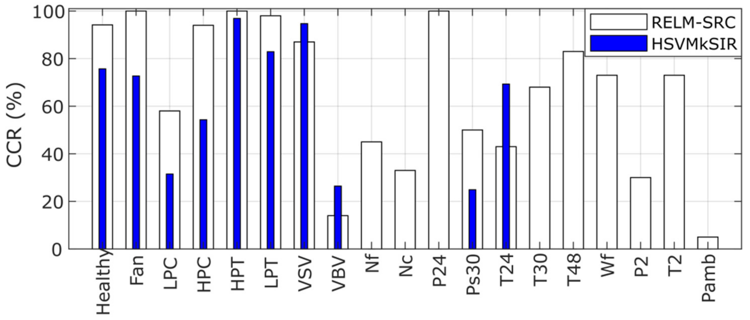
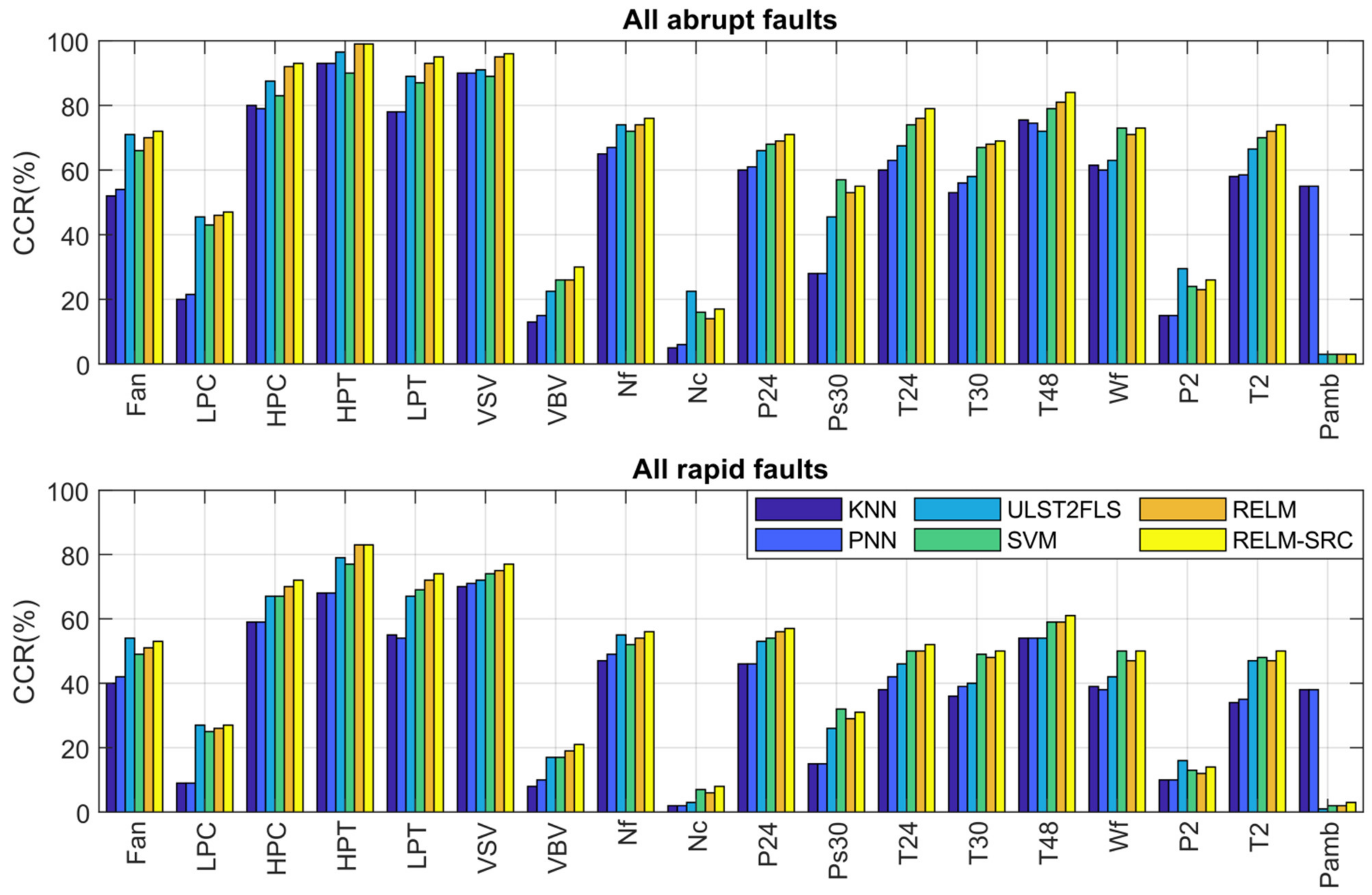
• As in the case of TPR, abrupt faults present higher CCR than rapid ones since the former are easier to detect.
• RELM-SRC wins in 12 rapid and 12 abrupt fault scenarios; the rest are draws and some wins with RELM, SVM, and ULST2-FLS.
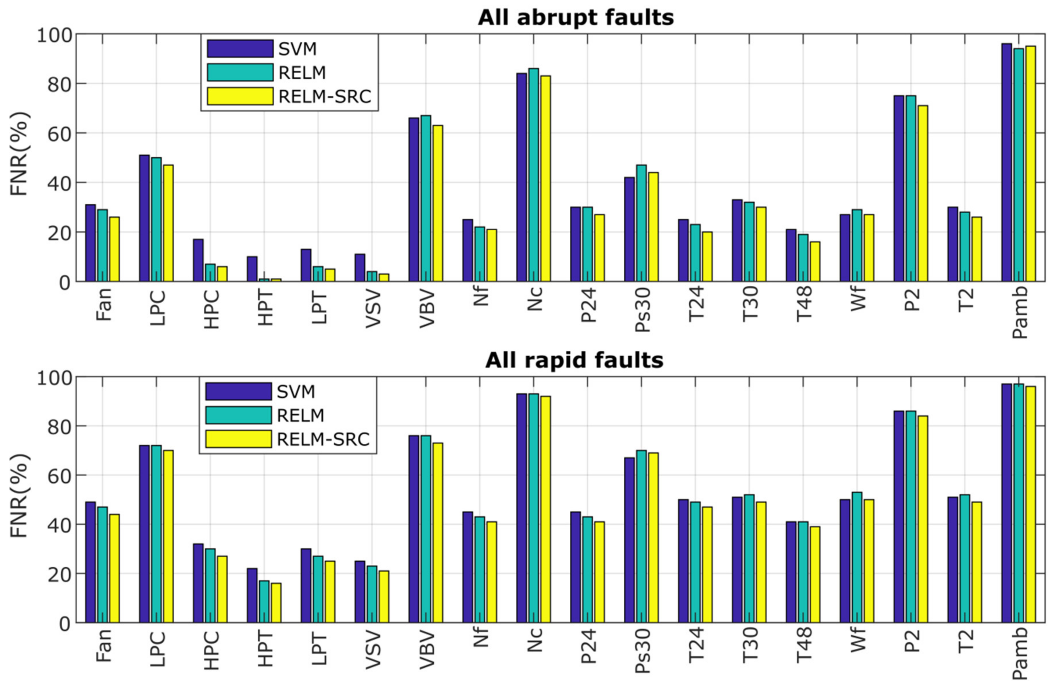
• The algorithms have problems identifying VBV actuator faults and three sensor faults related to Nc, P2, and Pamb, as also reported in papers [13,21]. Some present slightly better performance than others except for PNN and KNN, which effectively recognize the Pamb fault, but in general, the CCR values are low, especially for rapid faults. This identification problem occurs due to the nature of the faults and the possible combination of the following reasons:

  (a)

  The false-negative rate (FNR or omitted faults) and the false-positive rate (FPR or false alarms) are interconnected, i.e., when FNR reduces, FPR increases. This is precisely the case when the ProDiMES condition of false alarms (one false alarm per 1000 flights or FPR < 0.1%) is applied to the algorithm, increasing the probabilities of omitted faults. In other words, the column of FNR values in the confusion matrix contains a big number of incorrect diagnosis decisions due to the great influence of the no-fault class, demonstrating that the algorithm misclassifies the actual faults as healthy cases. Figure 9 displays the FNR for each rapid and abrupt fault class obtained by the three techniques. It is visible that Nc, P2, and especially Pamb have the highest FNR values (greater than 80%) since they are highly confused as the healthy class;

  (b)

  The low magnitudes assigned to these faults in ProDiMES affect the recognition task since the faults are contained in same the region of the healthy class, causing their misclassification as healthy cases; and

  (c)

  The problematic faults present low signal-to-noise ratios, and according to [13], the sensor noise levels averaged for an engine fleet and implemented in ProDiMES are much higher compared to other references that use the same type of turbofan engine, producing a significant challenge to correctly perform the diagnosis. Simon et al. [21] reported the use of additional logic to help improve the diagnosis in these fault scenarios, while in the case of [13], the improvement was associated with a fault detector based on calculated Mach value monitoring. The implementation of both types of approaches to increase the probabilities of these particular faults at expense of other classes is not the objective of the benchmarking analysis but to have a global performance (meeting the requirement of FPR < 0.1%). Thus, in general terms, it is neither an advantage for the algorithms in [13,21] nor a deficiency in our proposed methodology;

  (d)

  With other faults presenting FNR values of 50%, the total number of fault scenarios, the amount of testing samples, and the total level of fault classification accuracy is impacted negatively.

Continuing with the analysis of Table 11, MCR is computed as TPR minus CCR not considering the misclassifications due to the healthy class (omitted detections). From the table, one can see that the proposed algorithm reduces the misclassification rate by 1.04% in comparison with the third-best algorithm (PNN) and up to 6.78% with the last place (GE). RELM shows an MCR of 0 (averaged off-diagonal probability is negligible), and SVM and RELM-SRC are tied in second place with only 0.3%. Authors of WMFLS [25] did not report any value of MCR.

For detection latency, the difference between techniques is small. However, the proposed system detects faults 0.72 and 1.5 fight cycles sooner than those for the third (PATKF) and last place (WLS, KNN), respectively. Finally, as a reflection of global fault classification performance, RELM-SRC, RELM, and SVM win the first positions for the kappa coefficient. For example, RELM-SRC improves the performance in 0.038, 0.08, and 0.168 compared to ULST2-FLS, KNN, WMFLS, respectively.

5. Discussion

5.1. About the Stages of Comparison

The comparison section helped analyze the behavior of metrics and provided information about the diagnostic capabilities of the algorithms. The analysis became more objective and relevant from stage to stage. The first three stages allowed for adjusting the proposed algorithm and preparing it for the fourth stage, the blind test case.

Stage 1 enabled a preliminary comparison between techniques using different sizes of training datasets under the cruise regime. Additionally, smoothing in both training and testing deviations was considered to produce a significant increase in the diagnostic accuracy for all the techniques.

In Stage 2, the present study used the dataset provided in ProDiMES, while the authors in [8,22] generated their own test dataset. However, both types of sets were computed for the same engine, the same operating point, and the same structure of faults. For this reason, the differences between the sets cannot significantly change the algorithms’ performances and comparison results.

In Stage 3, the successive development of two versions of the algorithm, one-point and multipoint, had the following reasons. First, a simpler one-point version allowed a better adjustment of each algorithm element to debug the entire software. Second, the availability of a cruise version allowed the comparison of the proposed algorithm with known diagnostic solutions also using ProDiMES; such a comparison enabled a greater number of candidate algorithms and made the study more comprehensive.

The comparison in Stage 4 can be considered the most reliable because all the algorithms employed the same input data and passed through the blind test. However, the previous stages were also useful as far as they showed that none of the available information contradicts the superiority of RELM-SRC, nearly followed by RELM. Thus, one can state that the proposed framework has the best accuracy performances among all the diagnostic solutions that have been tested by ProDiMES so far.

5.2. About the Factors in the Algorithm That Contributed to the High Performance

The high performance achieved by the proposed system might be related to diverse factors that can be seen as clear advantages. First, in the majority of the compared frameworks, the faults are detected by an anomaly detection algorithm based on a threshold applied to a deviation vector length. Such a procedure provokes delays in diagnostic decisions, and the healthy engine class is limited in the diagnostic space by a decision boundary with a rigid form. In contrast, our algorithm computes anomaly detection and fault identification diagnostic at once by the same machine-learning technique and adapting the mentioned boundary to each fault. All the metrics confirm this, especially the detection latency.

Second, the hybrid scheme in RELM-SRC gives a second opportunity for the noisy samples to be reclassified with a noise-robust method to reduce the possibility to be misclassified as healthy cases or faults with small magnitude.

Third, the optimization of the proposed diagnostic algorithm is a complex process that requires taking into account not only the tuning of the machine-learning techniques but also all peculiarities and requirements of the ProDiMES methodology. For that reason, the algorithm was adjusted in each stage considering the optimal selection of the reference set for average baseline model and model correction; the size of the training dataset; the deviation smoothing coefficient; the internal parameters in the techniques (regularization parameter ${\xi }_{opt}$ and number of hidden neurons for RELM, threshold τ, and k in the adaptive sub-dictionary); and the number of healthy engines to meet the condition of no more than one false alarm per 1000 flights. As a result, the optimized algorithm produced a diagnostic accuracy $\overline{P}$ that is two times greater than the value of the algorithm from [28], and the number of healthy engines were reduced significantly from 14,000 to 2000 engines in the blind test case to meet the requirement of one false alarm per 1000 flights compared to paper [23].

5.3. About Some Advantages and Disadvantages of the Compared Fault Identification Techniques

The proposed hybrid approach has the advantage that the RELM block is simple to construct and fast to train. The SRC block does not have a training stage, and the use of adaptive sub-dictionaries (formed with training classes) instead of over-complete dictionaries helps to enhance signal sparse representation, reduce classification errors, and decrease testing time. However, a clear disadvantage is that RELM does not handle noisy signals well, producing misclassifications, and SRC based on sub-dictionaries still presents considerable computational costs.

Compared to WMFLS, which is based on a type-1 fuzzy logic system and considers up to 1814 rules extracted automatically, ULST2-FLS exploits the capabilities of the type-2 fuzzy logic system to model and deal with sensor uncertainties. The method works with max-product composition, product implication, Gaussian membership functions, and has the advantage of employing a reduced number of rules (76 rules) in the inference engine to classify the engine faults. In addition, ULST2-FLS reduces the training stage complexity by avoiding the Karnik–Mendel algorithm [24]. In general, the drawbacks in fuzzy logic systems are that the diagnostic accuracy depends on rules, which in turn are dependent on the knowledge and expertise of the subject expert, and also a great amount of training data and rules is required [7].

For the case of PNN, it is simple to construct, with low execution time, and has the advantage of providing probabilistic confidence with every diagnostic decision [13]. In a direct comparison with WLS, which is linear in nature and requires a fault influence matrix from a physics-based model, PNN is a data-driven method that captures the non-linear behavior of the system [21]. However, PNN yields to other ANNs in recognition accuracy and requires elevated computational resources when the number of samples is increased (the number of radial basis functions as hidden neurons increases in the same quantity) [23].

As for SVM, it has a good generalization performance with a small number of samples, it is not limited to the computational memory as in the case of PNN, and the technique has a unique and global solution in comparison with ANNs that struggle with multiple local minima. Nevertheless, one disadvantage of SVM is the elevated training time compared to ANNs when the number of samples is increased [12].

5.4. About Future Areas of Research

During the benchmarking process, we identified the following areas of research intended for improving the algorithm using ProDiMES in the future:

-

A more robust algorithm that reduces deviation errors through the adaptation of baseline models according to the current level of engine deterioration.

-

A more complete and integrated approach that considers all the stages of feature extraction, anomaly detection, fault identification, lifetime prediction, and fault-severity estimation.

-

The use of operating conditions along with monitored variables as inputs to the fault recognition technique to provide more information about the engine operation.

-

The need for a method addressing imbalanced fault classification.

6. Conclusions

In this paper, a gas turbine monitoring and diagnostic algorithm was developed and examined on the ProDiMES software. One of the new characteristics of this algorithm is the use of a hybrid approach that uses the advantages of extreme learning machines and sparse representation as well as simultaneous fault detection and identification by the same recognition technique. Such a structure of a diagnostic process and careful optimization of all of the diagnostic steps resulted in high algorithm performances. Four stages of comparison with all the other diagnostic solutions using the ProDiMES platform showed that the proposed algorithm has the highest diagnostic performance. These salient features make the algorithm a promising tool for real gas turbine monitoring systems. The paper describes the algorithm and its tuning in detail so that the reader can repeat the calculations and verify the results. We hope that this information and high performance of the algorithm proposed in the paper will stimulate the competition between diagnostic solutions and their further development.

References

1. Tahan, M.; Tsoutsanis, E.; Muhammad, M.; Abdul Karim, Z.A. Performance-based health monitoring, diagnostics and prognostics for condition-based maintenance of gas turbines: A review. Appl. Energy 2017, 198, 122–144. [Google Scholar] [CrossRef] [Green Version]
2. Oster, C.V.; Strong, J.S.; Zorn, K. Why airplanes crash: Causes of accidents worldwide. In Proceedings of the 51st Annual Transportation Research Forum, Arlington, VA, USA, 11–13 March 2010. [Google Scholar]
3. Kahn, M.; Nickelsburg, J. An Economic Analysis of U.S Airline Fuel Economy Dynamics from 1991 to 2015; National Bureau of Economic Research: Cambridge, MA, USA, 2016; pp. 1–34. [Google Scholar]
4. Zhao, N.; Wen, X.; Li, S. A review on gas turbine anomaly detection for implementing health management. In Proceedings of the ASME Turbo Expo 2016, Seoul, Korea, 13–17 June 2016; p. V001T22A009. [Google Scholar]
5. Zaccaria, V.; Rahman, M.; Aslanidou, I.; Kyprianidis, K. A Review of Information Fusion Methods for Gas Turbine Diagnostics. Sustainability 2019, 11, 6202. [Google Scholar] [CrossRef] [Green Version]
6. Volponi, A.J. Gas Turbine Engine Health Management: Past, Present, and Future Trends. J. Eng. Gas Turbines Power 2014, 136, 5. [Google Scholar] [CrossRef]
7. Fentaye, A.D.; Baheta, A.T.; Gilani, S.I.; Kyprianidis, K.G. A review on gas turbine gas-path diagnostics: State-of-the-art methods, challenges and opportunities. Aerospace 2019, 6, 83. [Google Scholar] [CrossRef] [Green Version]
8. Jaw, L.C.; Lee, Y.-J. Engine diagnostics in the eyes of machine learning. In Proceedings of the ASME Turbo Expo 2014: Turbine Technical Conference and Exposition, Düsseldorf, Germany, 16–20 June 2014; p. 8. [Google Scholar]
9. Li, Y.-G. Diagnostics of power setting sensor fault of gas turbine engines using genetic algorithm. Aeronaut. J. 2017, 121, 1109–1130. [Google Scholar] [CrossRef] [Green Version]
10. Fentaye, A.D.; Gilani, S.I.; Aklilu, B.T.; Mojahid, A. Two-shaft stationary gas turbine engine gas path diagnostics using fuzzy logic. J. Mech. Sci. Technol. 2017, 31, 5593–5602. [Google Scholar]
11. Hanachi, H.; Liu, J.; Mechefske, C. Multi-Mode Diagnosis of a Gas Turbine Engine Using an Adaptive Neuro-Fuzzy System. Chin. J. Aeronaut. 2018, 31, 1–9. [Google Scholar] [CrossRef]
12. Pérez-Ruiz, J.L.; Loboda, I.; Miró-Zárate, L.A.; Toledo-Velázquez, M.; Polupan, G. Evaluation of gas turbine diagnostic techniques under variable fault conditions. Adv. Mech. Eng. 2017, 9, 16. [Google Scholar] [CrossRef]
13. Koskoletos, A.O.; Aretakis, N.; Alexiou, A.; Romesis, C.; Mathioudakis, K. Evaluation of Aircraft Engine Gas Path Diagnostic Methods Through ProDiMES. J. Eng. Gas Turbines Power 2018, 140, 12. [Google Scholar] [CrossRef]
14. Lu, F.; Jiang, J.; Huang, J.; Qiu, X. Dual reduced kernel extreme learning machine for aero-engine fault diagnosis. Aerosp. Sci. Technol. 2017, 71, 742–750. [Google Scholar] [CrossRef]
15. Zhao, Y.P.; Huang, G.; Hu, Q.K.; Tan, J.F.; Wang, J.J.; Yang, Z. Soft extreme learning machine for fault detection of aircraft engine. Aerosp. Sci. Technol. 2019, 91, 70–81. [Google Scholar] [CrossRef]
16. Amare, D.F.; Aklilu, T.B.; Gilani, S.I. Gas path fault diagnostics using a hybrid intelligent method for industrial gas turbine engines. J. Braz. Soc. Mech. Sci. Eng. 2018, 40, 578. [Google Scholar] [CrossRef]
17. Xu, M.; Wang, J.; Liu, J.; Li, M.; Geng, J.; Wu, Y.; Song, Z. An improved hybrid modeling method based on extreme learning machine for gas turbine engine. Aerosp. Sci. Technol. 2020, 107, 106333. [Google Scholar] [CrossRef]
18. Togni, S.; Nikolaidis, T.; Sampath, S. A combined technique of Kalman filter, artificial neural network and fuzzy logic for gas turbines and signal fault isolation. Chin. J. Aeronaut. 2020, 34, 124–135. [Google Scholar] [CrossRef]
19. Simon, D.L.; Bird, J.; Davison, C.; Volponi, A.; Iverson, R.E. Benchmarking gas path diagnostic methods: A public approach. In Proceedings of the ASME Turbo Expo 2008, Berlin, Germany, 9–13 June 2008; pp. 325–336. [Google Scholar]
20. Simon, D.L. Propulsion Diagnostic Method Evaluation Strategy (ProDiMES) User’s Guide; National Aeronautics and Space Administration: Cleveland, OH, USA, 2010.
21. Simon, D.L.; Borguet, S.; Léonard, O.; Zhang, X. Aircraft engine gas path diagnostic methods: Public benchmarking results. J. Eng. Gas Turbines Power 2014, 136, 4. [Google Scholar] [CrossRef] [Green Version]
22. Borguet, S.; Leonard, O.; Dewallef, P. Regression-Based Modeling of a Fleet of Gas Turbine Engines for Performance Trending. J. Eng. Gas Turbines Power 2016, 138, 2. [Google Scholar] [CrossRef]
23. Loboda, I.; Pérez-Ruiz, J.L.; Yepifanov, S. A Benchmarking analysis of a data-driven gas turbine diagnostic approach. In Proceedings of the ASME Turbo Expo 2018, Oslo, Norway, 11–15 June 2018; p. V006T05A027. [Google Scholar]
24. Calderano, P.H.S.; Ribeiro, M.G.C.; Amaral, R.P.F.; Vellasco, M.M.B.R.; Tanscheit, R.; de Aguiar, E.P. An enhanced aircraft engine gas path diagnostic method based on upper and lower singleton type-2 fuzzy logic system. J. Braz. Soc. Mech. Sci. Eng. 2019, 41, 70. [Google Scholar] [CrossRef]
25. Teixeira, T.; Tanscheit, R.; Vellasco, M. Sistema de inferência fuzzy para diagnóstico de desempenho de turbinas a gás aeronáuticas. In Proceedings of the Fourth Brazilian Conference on Fuzzy Systems, Campinas, Brazil, 16–18 November 2016; pp. 242–253. [Google Scholar]
26. Frederick, D.K.; DeCastro, J.A.; Litt, J.S. User’s Guide for the Commercial Modular Aero-Propulsion System Simulation (C-MAPSS); National Aeronautics and Space Administration: Cleveland, OH, USA, 2007.
27. Loboda, I. Gas turbine diagnostics. In Efficiency, Performance and Robustness of Gas Turbines; InTech: Rijeka, Croatia, 2012; pp. 191–212. [Google Scholar]
28. Salvador, F.-A.; Felipe de Jesús, C.-A.; Igor, L.; Juan Luis, P.-R. Gas Turbine Diagnostic Algorithm Testing Using the Software ProDiMES. Ing. Investig. Tecnol. 2017, 18, 75–86. [Google Scholar]
29. Van Heeswijk, M.; Miche, Y. Binary/ternary extreme learning machines. Neurocomputing 2015, 149, 187–197. [Google Scholar] [CrossRef] [Green Version]
30. Timofte, R.; van Gool, L. Adaptive and Weighted Collaborative Representations for image classification. Pattern Recognit. Lett. 2014, 43, 127–135. [Google Scholar] [CrossRef] [Green Version]
31. Cao, J.; Zhang, K.; Luo, M.; Yin, C.; Lai, X. Extreme learning machine and adaptive sparse representation for image classification. Neural Netw. 2016, 81, 91–102. [Google Scholar] [CrossRef] [PubMed]
Figure 1. ProDiMES benchmarking process.
Aerospace 08 00232 g001
Figure 2. Deviations: (a) for a reference sample of 10 engines and their 90 first flights, (b) for baseline model verification with 1 engine through its service life.
Aerospace 08 00232 g002
Figure 3. Corrected and uncorrected deviations for different healthy engines.
Aerospace 08 00232 g003
Figure 4. The proposed hybrid fault classification procedure.
Aerospace 08 00232 g004
Figure 5. Recognition problem using feature vectors for (a) anomaly detection stage, (b) fault identification stage, and (c) both stages as a common process.
Aerospace 08 00232 g005
Figure 6. Correct classification rates of the proposed hybrid approach and the best technique from paper [8] for abrupt faults under cruise regime (Stage 2).
Aerospace 08 00232 g006
Figure 7. Variation of the number of training healthy engines in RELM-SRC to satisfy TNR ≥99.9% (Stage 3).
Aerospace 08 00232 g007
Figure 8. Correct classification rates for abrupt and rapid faults (Stage 4).
Aerospace 08 00232 g008
Figure 9. False-negative rate (omitted faults) of three techniques for abrupt and rapid faults (Stage 4).
Aerospace 08 00232 g009