
Probabilistic Flight Delay Predictions Using Machine Learning and Applications to the Flight-to-Gate Assignment Problem


Abstract
1. Introduction
2. Data-Driven Probabilistic Flight Delay Predictions
2.1. Data Description
2.1.1. Flight Schedule Dataset
2.1.2. Weather Dataset
2.2. Feature Selection
2.3. Machine-Learning Algorithms to Estimate the Probability Distribution of Flight Delays
2.3.1. Mixture Density Networks (MDNs)
2.3.2. Random Forests Regression and Kernel Density Estimation
2.4. Hyperparameter Tuning
2.5. Performance Metrics for Probabilistic Forecasting
2.5.1. Continuous Ranked Probability Score
2.5.2. and
2.5.3. Metrics Based on the Standard Deviation
2.6. Results—Probabilistic Flight Delay Predictions
2.7. Impact of the Choice of the Hyperparameters
3. Integrating Probabilistic Delay Predictions into the Flight-to-Gate Assignment Problem
3.1. Mathematical Formulation of the Deterministic FGAP Model
3.2. Mathematical Formulation of the Probabilistic FGAP
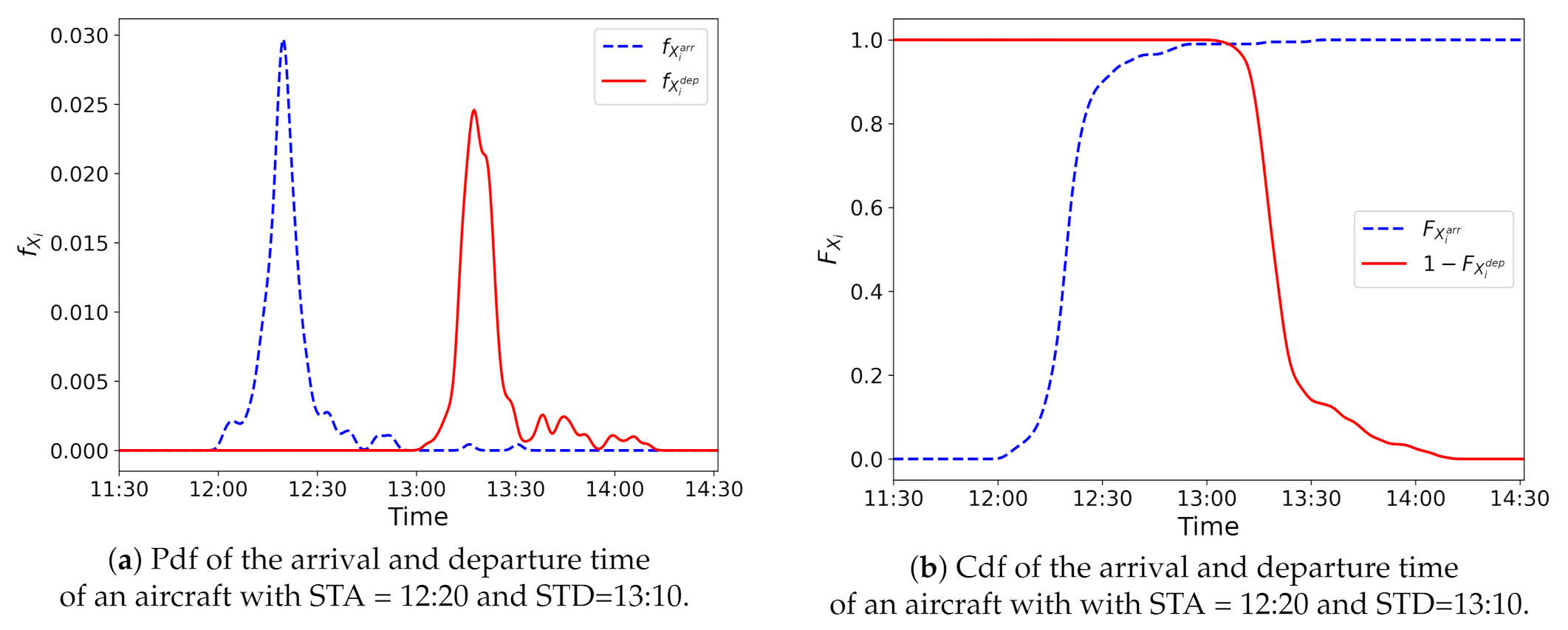
3.3. Aircraft Presence Probability Function
3.4. Results—Flight-to-Gate-Assignment Integrating Probabilistic Flight Delay Predictions
3.5. Results—Long Run Performance
- An aircraft is defined as a conflicted aircraft if there is at least one time slot at which this aircraft and any other aircraft are both present at the same gate.
- For the probabilistic FGAP model, a gate time slot is defined as a used gate time slot if there is an aircraft present at the gate at this time with a probability of more than —for the deterministic FGAP model, if there is an aircraft present at the gate at this time. Note that the maximum amount of used gate time slots is equal to .
4. Conclusions
Author Contributions
Funding
Institutional Review Board Statement
Informed Consent Statement
Data Availability Statement
Conflicts of Interest
Abbreviations
| RTM | Rotterdam The Hague Airport |
| MDN | Mixture Density Networks |
| RFR | Random Forests Regression |
| FGAP | Flight-to-Gate Assignment Problem |
| MAE | Mean Absolute Error |
| RMSE | Root Mean Squared Error |
| CRPS | Continuous Ranked Probability Score |
| KDE | Kernel Density Estimation |
| CA | Conflicted Aircraft |
| UGT | Used Gate Time slots |
| Probability Density Function | |
| cdf | Cumulative Distribution Function |
References
- Eurocontrol Network Manager Annual Report. 2019. Available online: https://www.eurocontrol.int/publication/network-manager-annual-report-2019 (accessed on 24 February 2021).
- Eurocontrol Annual Network Operations Report. 2019. Available online: https://www.eurocontrol.int/publication/annual-network-operations-report-2019 (accessed on 24 February 2021).
- Eurocontrol Five-Year Forecast 2020–2024. Available online: https://www.eurocontrol.int/publication/eurocontrol-five-year-forecast-2020-2024 (accessed on 24 February 2021).
- Kim, Y.J.; Choi, S.; Briceno, S.; Mavris, D. A deep learning approach to flight delay prediction. In Proceedings of the AIAA/IEEE Digital Avionics Systems Conference, Sacramento, CA, USA, 25–29 September 2016; pp. 1–6. [Google Scholar] [CrossRef]
- Lambelho, M.; Mitici, M.; Pickup, S.; Marsden, A. Assessing strategic flight schedules at an airport using machine learning-based flight delay and cancellation predictions. J. Air Transp. Manag. 2020, 82, 101737. [Google Scholar] [CrossRef]
- Choi, S.; Kim, Y.J.; Briceno, S.; Mavris, D. Prediction of Weather-Induced Airline Delays Based on Machine Learning Algorithms. In Proceedings of the IEEE/AIAA 35th Digital Avionics Systems Conference (DASC), Sacramento, CA, USA, 25–29 September 2016. [Google Scholar] [CrossRef]
- Alonso, H.; Loureiro, A. Predicting flight departure delay at Porto Airport: A preliminary study. In Proceedings of the 2015 7th International Joint Conference on Computational Intelligence (IJCCI), Lisbon, Portugal, 12–14 November 2015; IEEE: New York, NY, USA, 2015; Volume 3, pp. 93–98. [Google Scholar]
- Chen, J.; Li, M. Chained predictions of flight delay using machine learning. In Proceedings of the AIAA Scitech 2019 Forum, San Diego, CA, USA, 7–11 January 2019; pp. 1–25. [Google Scholar] [CrossRef]
- Kalliguddi, A.M.; Leboulluec, A.K. Predictive Modeling of Aircraft Flight Delay. Univers. J. Manag. 2017, 5, 485–491. [Google Scholar] [CrossRef]
- Manna, S.; Biswas, S.; Kundu, R.; Rakshit, S.; Gupta, P.; Barman, S. A statistical approach to predict flight delay using gradient boosted decision tree. In Proceedings of the ICCIDS 2017—International Conference on Computational Intelligence in Data Science, Chennai, India, 2–3 June 2018; pp. 1–5. [Google Scholar] [CrossRef]
- Yu, B.; Guo, Z.; Asian, S.; Wang, H.; Chen, G. Flight delay prediction for commercial air transport: A deep learning approach. Transp. Res. Part E Logist. Transp. Rev. 2019, 125, 203–221. [Google Scholar] [CrossRef]
- Thiagarajan, B.; Srinivasan, L.; Sharma, A.V.; Sreekanthan, D.; Vijayaraghavan, V. A machine learning approach for prediction of on-time performance of flights. In Proceedings of the AIAA/IEEE Digital Avionics Systems Conference, St. Petersburg, FL, USA, 17–21 September 2017; pp. 5–10. [Google Scholar] [CrossRef]
- Ayhan, S.; Costas, P.; Samet, H. Predicting estimated time of arrival for commercial flights. In Proceedings of the 24th ACM SIGKDD International Conference on Knowledge Discovery & Data Mining, Data Mining, London, UK, 19–23 August 2018; pp. 33–42. [Google Scholar]
- Shao, W.; Prabowo, A.; Zhao, S.; Tan, S.; Koniusz, P.; Chan, J.; Hei, X.; Feest, B.; Salim, F.D. Flight delay prediction using airport situational awareness map. In Proceedings of the GIS: Proceedings of the ACM International Symposium on Advances in Geographic Information Systems, Chicago, IL, USA, 5–8 November 2019; pp. 432–435. [Google Scholar] [CrossRef]
- Mueller, E.; Chatterji, G. Analysis of aircraft arrival and departure delay characteristics. In Proceedings of the AIAA’s Aircraft Technology, Integration, and Operations (ATIO) 2002 Technical Forum, Los Angeles, CA, USA, 1–2 October 2002; p. 5866. [Google Scholar]
- Novianingsih, K.; Hadianti, R. Modeling flight departure delay distributions. In Proceedings of the 2014 International Conference on Computer, Control, Informatics and Its Applications (IC3INA), Bandung, Indonesia, 21–23 October 2014; IEEE: New York, NY, USA, 2014; pp. 30–34. [Google Scholar]
- Itoh, E.; Mitici, M. Queue-based modeling of the aircraft arrival process at a single airport. Aerospace 2019, 6, 103. [Google Scholar] [CrossRef]
- Kleinbekman, I.C.; Mitici, M.; Wei, P. Rolling-Horizon Electric Vertical Takeoff and Landing Arrival Scheduling for On-Demand Urban Air Mobility. J. Aerosp. Inf. Syst. 2020, 17, 150–159. [Google Scholar] [CrossRef]
- Tu, Y.; Ball, M.O.; Jank, W.S. Estimating flight departure delay distributions—A statistical approach with long-term trend and short-term pattern. J. Am. Stat. Assoc. 2008, 103, 112–125. [Google Scholar] [CrossRef]
- Şeker, M.; Noyan, N. Stochastic optimization models for the airport gate assignment problem. Transp. Res. Part E Logist. Transp. Rev. 2012, 48, 438–459. [Google Scholar] [CrossRef]
- Van Schaijk, O.R.; Visser, H.G. Robust flight-to-gate assignment using flight presence probabilities. Transp. Plan. Technol. 2017, 40, 928–945. [Google Scholar] [CrossRef]
- L’Ortye, J.; Mitici, M.; Visser, H.G. Robust flight-to-gate assignment with landside capacity constraints. Transp. Plan. Technol. 2021, 44, 1–22. [Google Scholar] [CrossRef]
- Iowa State University. ASOS-AWOS-METAR Data Download. 2020. Available online: https://mesonet.agron.iastate.edu/request/download.phtml (accessed on 1 March 2020).
- Bishop, C.M. Mixture Density Networks. 1994. Available online: http://publications.aston.ac.uk/id/eprint/373/ (accessed on 14 July 2020).
- Schuster, M. Better Generative Models for Sequential Data Problems: Bidirectional Recurrent Mixture Density Networks. In Proceedings of the Advances in Neural Information Processing Systems, Denver, CO, USA, 29 November–4 December 1999; pp. 589–595. [Google Scholar]
- Zen, H.; Senior, A. Deep mixture density networks for acoustic modeling in statistical parametric speech synthesis. In Proceedings of the 2014 IEEE International Conference on Acoustics, Speech and Signal Processing (ICASSP); IEEE: New York, NY, USA, 2014; pp. 3844–3848. [Google Scholar]
- Xu, J.; Rahmatizadeh, R.; Bölöni, L.; Turgut, D. Real-time prediction of taxi demand using recurrent neural networks. IEEE Trans. Intell. Transp. Syst. 2017, 19, 2572–2581. [Google Scholar] [CrossRef]
- Carney, M.; Cunningham, P.; Dowling, J.; Lee, C. Predicting Probability Distributions for Surf Height Using an Ensemble of Mixture Density Networks. In Proceedings of the 22nd international conference on Machine learning, Bonn, Germany, 7–11 August 2005. [Google Scholar]
- Vossen, J.; Feron, B.; Monti, A. Probabilistic Forecasting of Household Electrical Load Using Artificial Neural Networks. In Proceedings of the 2018 IEEE International Conference on Probabilistic Methods Applied to Power Systems (PMAPS), Boise, ID, USA, 24–28 June 2018; pp. 1–6. [Google Scholar]
- Felder, M.; Kaifel, A.; Graves, A. Wind power prediction using mixture density recurrent neural networks. Eur. Wind Energy Conf. Exhib. 2010, 5, 3417–3424. [Google Scholar]
- Zhang, J.; Yan, J.; Infield, D.; Liu, Y.; Lien, F.s. Short-term forecasting and uncertainty analysis of wind turbine power based on long short-term memory network and Gaussian mixture model. Appl. Energy 2019, 241, 229–244. [Google Scholar] [CrossRef]
- Breiman, L. Random forests. Mach. Learn. 2001, 45, 5–32. [Google Scholar] [CrossRef]
- Zhang, L.; Xie, L.; Han, Q.; Wang, Z.; Huang, C. Probability Density Forecasting of Wind Speed Based on Quantile Regression and Kernel Density Estimation. Energies 2020, 13, 6125. [Google Scholar] [CrossRef]
- Förster, S.; Schultz, M.; Fricke, H. Probabilistic Prediction of Separation Buffer to Compensate for the Closing Effect on Final Approach. Aerospace 2021, 8, 29. [Google Scholar] [CrossRef]
- Schlosser, L.; Hothorn, T.; Stauffer, R.; Zeileis, A. Distributional regression forests for probabilistic precipitation forecasting in complex terrain. arXiv 2018, arXiv:1804.02921. [Google Scholar] [CrossRef]
- Rahman, R.; Haider, S.; Ghosh, S.; Pal, R. Design of probabilistic random forests with applications to anticancer drug sensitivity prediction. Cancer Inform. 2015, 14, CIN-S30794. [Google Scholar] [CrossRef]
- Matheson, J.E.; Winkler, R.L. Scoring rules for continuous probability distributions. Manag. Sci. 1976, 22, 1087–1096. [Google Scholar] [CrossRef]
- Gneiting, T.; Katzfuss, M. Probabilistic forecasting. Annu. Rev. Stat. Its Appl. 2014, 1, 125–151. [Google Scholar] [CrossRef]
- Daş, G.S.; Gzara, F.; Stützle, T. A review on airport gate assignment problems: Single versus multi objective approaches. Omega 2020, 92, 102146. [Google Scholar] [CrossRef]
- Ascó, A. Steady State Evolutionary Algorithm and Operators for the Airport Gate Assignment Problem. Int. J. Adv. Robot Automn. 2019, 4, 24. [Google Scholar] [CrossRef]
- Mangoubi, R.S. A Linear Programming Solution to the Gate Assignment Problem. 1980. Available online: https://dspace.mit.edu/handle/1721.1/67926 (accessed on 29 August 2020).
- Yu, C.; Zhang, D.; Lau, H.Y. MIP-based heuristics for solving robust gate assignment problems. Comput. Ind. Eng. 2016, 93, 171–191. [Google Scholar] [CrossRef]
- Kim, S.H.; Feron, E.; Clarke, J.P.; Marzuoli, A.; Delahaye, D. Airport gate scheduling for passengers, aircraft, and operations. J. Air Transp. 2017, 25, 109–114. [Google Scholar] [CrossRef]


| Prediction | Features |
|---|---|
| Departure delay | Airport a, Airline a, Season a, Time of day b, Day of week b, Day of month b, Day of year b, Airport latitude c, Airport longitude c, Day of month c, Seats c, Year c, Scheduled flights 2 h c, Scheduled flights day c, Dewpoint c, Visibility c, Pressure c, Wind speed c |
| Arrival delay | Airport a, Airline a, Aircraft type a, Season a, Time of day b, Day of week b, Day of month b, Month b, Airport longitude c, Day of month c, Distance c, Seats c, Year c, Scheduled flights 2h c, Scheduled flights day c, Temperature c, Visibility c, Pressure c, Wind speed c |
| Feature | Description |
|---|---|
| Airport | the airport of destination (departures) or origin (arrivals) |
| Airline | the airline operating the flight |
| Aircraft type | the aircraft type used for the flight |
| Season | the flight season (summer or winter schedule) |
| Time of day | scheduled time of day of the flight |
| Day of week | scheduled day of the week of the flight |
| Day of month | scheduled day of the month of the flight |
| Day of year | scheduled day of the year of the flight |
| Month | scheduled month number of the flight |
| Airport latitude and longitude | the latitude and longitude of the destination/origin airport |
| Distance | the distance between the origin and destination |
| Seats | the seat capacity of the used aircraft |
| Year | the year in which the flight was operated |
| Temperature | the air temperature at the destination/origin airport |
| Dewpoint | the dewpoint temperature at the destination/origin airport |
| Visibility | the prevailing visibility at the destination/origin airport |
| Pressure | pressure altimeter at the destination/origin airport |
| Wind speed | wind speed at the destination/origin airport |
| Scheduled flights day | the number of flights scheduled to depart/arrive during the day of the flight |
| Scheduled flights 2h | the number of flights scheduled to depart/arrive during the period between one hour before and one hour after the scheduled time of the flight |
| Mixture Density Network | ||
|---|---|---|
| Hyperparameter | Value | Range |
| Number of modes m | 8 | [3, 5, 8, 10, 15] |
| Number of hidden layers | 3 | [1, 2, 3] |
| Number of nodes per hidden layer | 50 | [25, 50, 75, 100] |
| Number of epochs | 1000 | [500, 750, 1000, 1250, 1500] |
| Random Forest Regression | ||
| Hyperparameter | Value | Range |
| Number of estimators | 200 | [100, 150, 200, 300] |
| Split criterion | Mean-squared error | [MSE, MAE] |
| Maximum tree depth | 20 | [4, 6, 8, 10, 12, 15, 20, 30] |
| Minimum samples per leaf node | 7 | [0, 3, 5, 7, 9] |
| Fraction of features considered for split | 0.75 | [0.25, 0.50, 0.75, 1.00] |
| KDE Bandwidth h | 1.5 | [0.5, 1, 1.5, 2] |
| Flights | Algorithm | CRPS Mean | CRPS Std | ||||
|---|---|---|---|---|---|---|---|
| Departures | MDN | 9.12 | 19.15 | 13.23 | 24.23 | 23.85 | 0.92 |
| RFR | 8.86 | 18.15 | 12.51 | 23.32 | 12.08 | 0.69 | |
| Arrivals | MDN | 10.95 | 17.59 | 15.62 | 24.98 | 24.60 | 0.87 |
| RFR | 10.85 | 17.49 | 14.99 | 24.39 | 14.02 | 0.61 |
| CA Mean | CA | UGT Mean | UGT | |
|---|---|---|---|---|
| Total | 31.6 | 6.7 | 2304 | N/A |
| Deterministic FGAP | 5.03 | 2.87 | 254 | 57.9 |
| Probabilistic FGAP, r = 0.15 | 2.57 | 2.30 | 319 | 76.7 |
| Probabilistic FGAP, r = 0.10 | 1.73 | 1.84 | 319 | 76.5 |
| Probabilistic FGAP, r = 0.05 | 1.33 | 1.49 | 319 | 76.6 |
Publisher’s Note: MDPI stays neutral with regard to jurisdictional claims in published maps and institutional affiliations. |
© 2021 by the authors. Licensee MDPI, Basel, Switzerland. This article is an open access article distributed under the terms and conditions of the Creative Commons Attribution (CC BY) license (https://creativecommons.org/licenses/by/4.0/).
Share and Cite
Zoutendijk, M.; Mitici, M. Probabilistic Flight Delay Predictions Using Machine Learning and Applications to the Flight-to-Gate Assignment Problem. Aerospace 2021, 8, 152. https://doi.org/10.3390/aerospace8060152
Zoutendijk M, Mitici M. Probabilistic Flight Delay Predictions Using Machine Learning and Applications to the Flight-to-Gate Assignment Problem. Aerospace. 2021; 8(6):152. https://doi.org/10.3390/aerospace8060152
Chicago/Turabian StyleZoutendijk, Micha, and Mihaela Mitici. 2021. "Probabilistic Flight Delay Predictions Using Machine Learning and Applications to the Flight-to-Gate Assignment Problem" Aerospace 8, no. 6: 152. https://doi.org/10.3390/aerospace8060152
APA StyleZoutendijk, M., & Mitici, M. (2021). Probabilistic Flight Delay Predictions Using Machine Learning and Applications to the Flight-to-Gate Assignment Problem. Aerospace, 8(6), 152. https://doi.org/10.3390/aerospace8060152