Article

Load-Identification Method for Flexible Multiple Corrugated Skin Using Spectra Features of FBGs

1
State Key Laboratory of Mechanics and Control of Mechanical Structures, Nanjing University of Aeronautics and Astronautics, Nanjing 210000, China
2
College of Civil Aviation, Nanjing University of Aeronautics and Astronautics, Nanjing 210000, China
*
Author to whom correspondence should be addressed.
Aerospace 2021, 8(5), 134; https://doi.org/10.3390/aerospace8050134
Submission received: 27 March 2021 / Revised: 28 April 2021 / Accepted: 5 May 2021 / Published: 9 May 2021

Abstract

:
Flexible corrugated skins are ideal structures for morphing wings, and the associated load measurements are of great significance in structural health monitoring. This paper proposes a novel load-identification method for flexible corrugated skins based on improved Fisher discrimination dictionary learning (FDDL). Several fiber Bragg grating sensors are pasted on the skin to monitor the load on multiple corrugated crests. The loads on different crests cause nonuniform strain fields, and these discriminative spectra are recorded and used as training data. The proposed method involves load-positioning and load-size identification. In the load-size-identification stage, a classifier is trained for every corrugated crest. An interleaved block grouping of samples is introduced to enhance the discrimination of dictionaries, and a two-resolution load-size classifier is introduced to improve the performance and resolution of the grouping labels. An adjustable weight is introduced to the FDDL classification scheme to optimize the contribution from different sensors for different load-size classifiers. With the proposed method, the individual loads on eight crests can be identified by two fiber Bragg grating sensors. The positioning accuracy is 100%, and the mean error of the load-size identification is 0.2106 N, which is sufficiently precise for structural health monitoring.

1. Introduction

Flexible composite corrugated skin materials exhibit different mechanical behaviors in different directions, typically having satisfactory load-bearing ability in the transverse direction and cumulative deformation in the chord direction [1,2]. These characteristics meet the requirements of aircraft wing structures, so corrugated skins are regarded as ideal materials for morphing wings [3]. Composite laminate materials are easily delaminated, cracked and degummed under complex loading [4,5,6]. Specific to flexible corrugated skins, loading perpendicular to the crest will damage the structure and reduce the load-bearing capacity, deformation capacity, and reliability. Therefore, identifying the load on the corrugated skin is of great significance for structural health monitoring (SHM) [7,8].
Research on flexible composite skins has mainly focused on tensile and deformation properties, which are usually measured by force sensors of test machines or some noncontact displacement measurement techniques [9,10]. Ghabezi simulated the mechanical characteristics of trapezoidal corrugated composite skins and verified them by experiment. In his research, mechanical properties were obtained by the force sensors on the INSTRON 5500 machine [11]. In Yokozeki’s research of morphing airfoil using a corrugated structure, deformations were measured by VIVID910, which is a noncontact laser scanning device [12]. Digital image correlation and vision measurement techniques are also popular in the measurement of deformed states of corrugated skins [13]. There are relatively few studies on the load identification and damage detection of flexible corrugated skins with pasted sensors in aerospace applications. However, there have been some studies on the measurement of corrugated structures applied in the field of construction and bridges.
Brachman tested deep corrugated steel culverts to gain the deflections and strains of this structure with several electrical foil resistance strain gauges pasted evenly on the corrugations [14]. In terms of the dynamic measurement of corrugated structures, Manko obtained the dynamic coefficients, vibration velocity, and vibration frequency of the target structure by pasting sensors to the corrugated steel plates in a bridge [15]. The mechanical properties of the pasted positions are monitored by attaching sensors to a bridge structure using corrugated steel plates, and the damping decrements and damping ratios of the culvert were determined through a fast Fourier transform [16]. The sensors were pasted at the crests of the corrugated structures in their researches, the target structures were relatively large, and the number of corrugations was small, meaning there was sufficient space for placing the sensors on every crests which needed to be monitored. However, flexible corrugated skins on aircrafts typically have a small size and numerous corrugations, so the number and position of sensors are restricted. A method that uses a small number of sensors to monitor the load on multiple corrugations will effectively expand SHM applications of this type of material structure.
With the advantages of anti-electromagnetic interference and an integrated sensing and transmission function, fiber Bragg grating (FBG) sensors can be deployed on various target structures in many harsh environments. Thus, they are widely used in the measurement of aerospace structures [17,18,19]. When the FBG is affected by a nonuniform strain, complex changes in the FBG reflection spectrum can be measured by a spectrum analyzer [20,21]. At this time, the signal measured by the FBG is a one-dimensional vector, which contains plentiful original features [22]. Zhang combined finite element analysis with an FBG reflection spectrum simulation technique to predict the spectral signal of a damaged flexible corrugated skin [23]. An FBG sensor was pasted on the corrugated crest, and finite element analysis was used to obtain the strain field of the sensor just prior to the damage occurring. The simulation spectrum was then calculated and compared with the actual spectrum. This allowed the relationship between the reflection spectrum and the tensile load to be established.
As the loads at different positions have different magnitudes, the strain fields at each FBG position are different. The corresponding spectra with different positions and different load sizes are unique. Therefore, the reflection spectra are discriminative and could be used as training data, enabling the identification of the load position and load size through machine learning algorithms. This is the premise that the load identification target can be achieved through machine learning methods. In the method proposed in this paper, training data are obtained by two FBG sensors pasted on a flexible corrugated skin specimen. Both the load position and the load size need to be identified. A load-position classifier (LPC) is trained by samples from the same crest as belonging to the same class. The load-size classifiers (LSCs) are separately trained for different load crests. In the test phase, the load is first located by the LPC, and then the corresponding LSC is used to identify the load size.
Sparse representation (SR) has achieved great success in signal restoration, compressed sensing, and pattern recognition [24,25,26]. Using an SR algorithm, high-dimensional signals can be represented by a matrix called an overcomplete dictionary or dictionary. When the coding coefficients or reconstruction error of SR are related to the class labels of samples, the SR algorithm can be used as a classifier [27]. There are three elements that affect the recognition performance of SR algorithms: (i) dictionary composition; (ii) dictionary learning (DL); and (iii) representation algorithms [28,29,30]. The method proposed in this paper focuses on improving the dictionary composition and DL under the scenario of corrugated skin load identification.
In common SR applications such as face recognition, training sample sets are generally databases of facial pictures [31]. In such databases, test samples usually show clustered distributions. The samples of the same person are naturally gathered as a class group. The similarity of samples in the same class and the distinction between different classes are the prerequisites for realizing the function of pattern recognition. In the load-positioning step, samples from the same corrugated crest are naturally grouped. In the load-size identification stage, however, this distribution of samples is not completely applicable. The increased step size of the load corresponding to the training samples in the training set is even, which means the samples lack clear barriers between groups. Such samples might cause two problems: (a) There is no natural grouping mode for the samples. If the sample grouping is too dense, it will affect the result of DL, whereas if it is too sparse, it will affect the resolution of the class labels. (b) The samples are grouped with a uniform load-size range, which will reduce the discrimination of the dictionary. To solve problem (a), this paper describes a two-resolution LSC. The groups identified by LSC1 are large, and the results from LSC1 indicate the sample sets of LSC2 that have higher resolutions. To solve problem (b), an interleaved block grouping model is introduced, in which the groups are interleaved into two occluding dictionaries. Under this dictionary composition, the distance between groups increases, and the discrimination of the dictionaries is significantly improved.
The proposed method is based on the Fisher discrimination dictionary learning (FDDL) algorithm, which is a supervised DL algorithm [32,33]. The discrimination of sub-dictionaries and the coefficient matrix are considered in the optimization of DL. FDDL can effectively improve the classification performance during the training process and has excellent performance in classification.
There are two FDDL classification schemes: a local classifier (LC) and a global classifier (GC). The LC is suitable for situations in which the group size is large, that is, the LPC in this study. The GC is suitable for cases in which there are few samples in the same group and can be used as an LSC. When collecting training samples for this study, it was discovered that the sensitivities of the two FBG sensors to loads at different crests were quite different. If the sensitivities of different sensors are considered in LSCs, the performance of the LSCs can be improved by introducing an adjustable weight to the LSC discriminants.

2. Background

2.1. Uniform Strain Sensing of the FBG

The center wavelength of a FBG reflection spectrum in the initial state is at the Bragg grating wavelength λ B and described as [34]:
λ B = 2 n e f f Λ ,
where Λ is the grating period and n e f f is the effective refractive index.
When only considering uniform changes in the axial strain, the optical fiber’s grating area will produce elastic-optical effects due to expansion and contraction. The elastic-optical effects will cause Λ and n e f f to change. The change in the grating period is shown as:
Δ Λ Λ = ε ,
where ε is the axial strain of the FBG, and the change in the effective refractive index is written as:
Δ n e f f n e f f = n e f f 2 [ P 12 υ ( P 11 P 12 ) ] 2 ε ,
where P 11 and P 12 are the elastic-optical coefficients and υ is Poisson’s ratio for the material. Combined with Equation (2), the shift of λ B is described as:
Δ λ B λ B = { 1 n e f f 2 2 [ P 12 υ ( P 11 + P 12 ) ] } ε .
Defining ( n e f f 2 / 2 ) [ P 12 υ ( P 11 + P 12 ) ] as the effective elasticity coefficient P e , Equation (4) can be simplified as:
Δ λ B λ B = { 1 P e } ε .
It can be seen that, under the influence of a uniform axial strain, the change in the center wavelength of the FBG, Δ λ B , has a linear relationship with the strain ε .

2.2. Nonuniform Strain Sensing of the FBG

There are two primary methods of analyzing FBGs under nonuniform strain, namely coupled-mode theory and transfer matrix (T-matrix) theory [35]. In this article, T-matrix theory was chosen to describe the nonuniform strain sensing of FBGs.
In T-matrix theory, the grating is divided into many sub-segments, each of which is subject to a uniform strain ε . The transmission characteristics for each sub-segment are obtained through coupling-mode theory. The amplitudes of the forward- and backward-propagating modes in the sub-segments are then obtained through the transmission matrix method and shown as:
[ R i S i ] = F i [ R i 1 S i 1 ] ,
where R i and S i are the field amplitudes after traversing the i th segment, and the transfer matrix F i is described as:
F i = [ cos h ( γ i Δ z ) i σ ^ γ i sin h ( γ i Δ z ) i k γ i sin h ( γ i Δ z ) i k γ i sin h ( γ i Δ z ) cos h ( γ i Δ z ) + i σ ^ γ i sin h ( γ i Δ z ) ] ,
where γ i = κ 2 σ ^ 2 , κ is the ac coupling coefficient, σ ^ is the dc self-coupling coefficient, and Δ z is the length of the sub-segment. The entire grating under a nonuniform strain can be described as-
[ R N S N ] = F [ R 0 S 0 ] ,
where F = F N F N 1 F i F 1 .
Equation (8) is the transmission characteristics of the entire sensor at the corresponding wavelength. When the transmission characteristics are calculated for all the sensing wavelength ranges, the reflection characteristics of the whole FBG can be obtained. Each strained optical-fiber sub-segment will affect the reflection spectrum signal of the FBG; therefore, the reflection spectrum signal of the FBG sensing will produce corresponding changes according to different nonuniform strain fields. This complex change of reflection spectrum will provide a wealth of discriminative information.

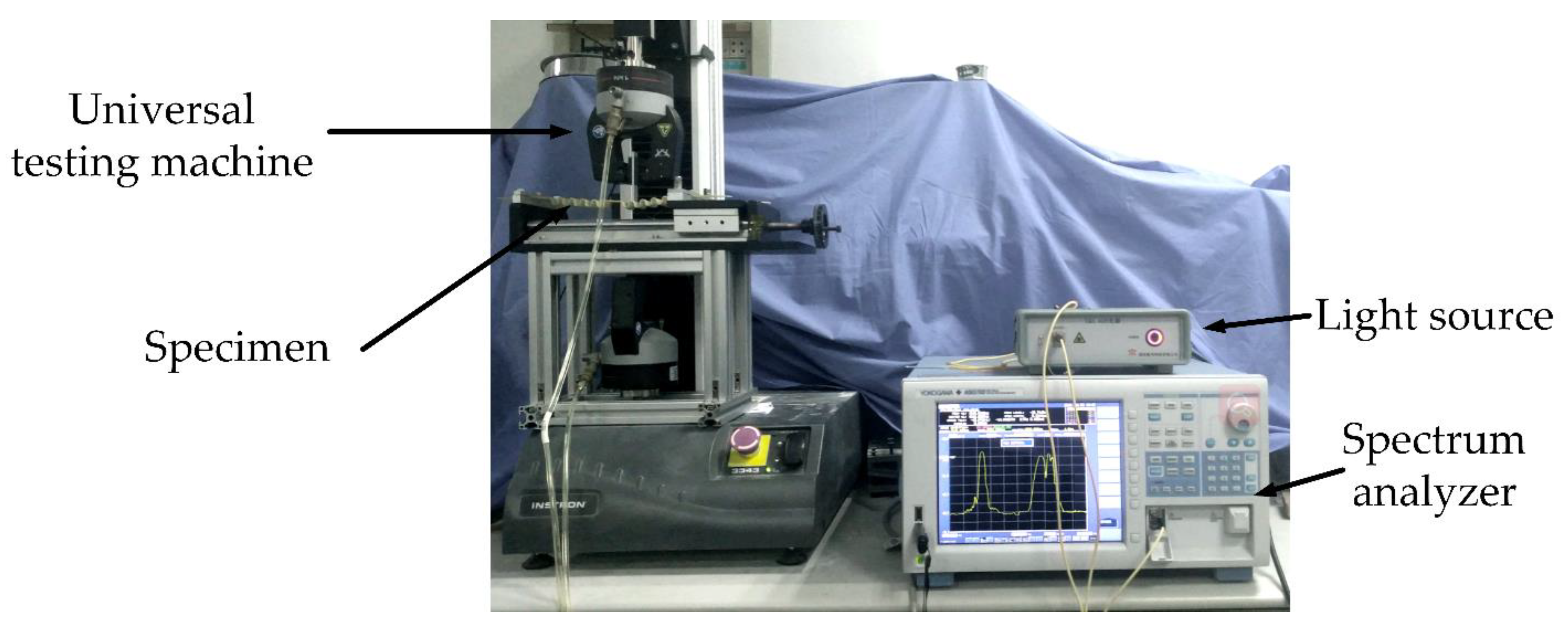
3. Experimental Setup

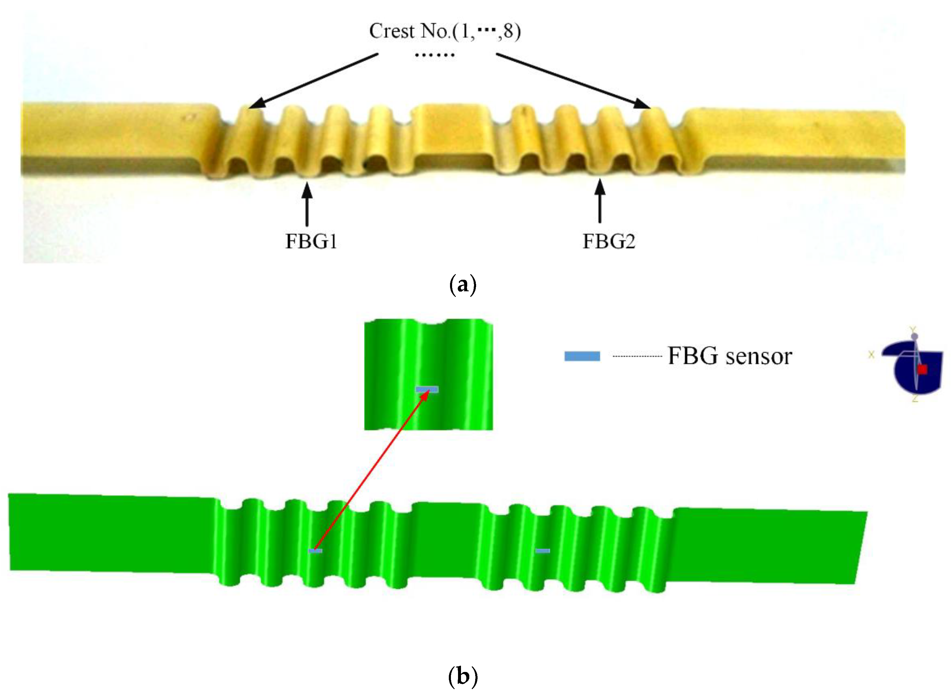
3.1. Specimen Analysis

The reinforcement of the composite specimen in this research was an E-type 0/90 glass fiber cloth, and the matrix of the specimen was a mixture of WSR6101 epoxy resin and low-molecular-weight 650-polyamide resin. The size parameters of the specimen are listed in Table 1.
In Table 1, l 1 is the length of the specimen in the chord direction, l 2 is the width in the transverse direction, l 3 is the radius of the corrugations, l 4 is the thickness of the specimen, and n 1 is the number of layers. The test specimen is pictured in Figure 1, and the material properties of specimen are shown in Table 2.
E 11 and E 22 are the elastic modulus of material in the chord and transverse directions, respectively, ρ is the density, C f is the mass ratio of glass fiber cloth, C m is the mass ratio of WSR6101 epoxy resin, and v 12 is the poisson’s ratio of the material.
Figure 1 indicates that the specimen has two continuous corrugations and is symmetrical in the chord direction. FBG1 is pasted at the center of back side crest 3, and FBG2 is pasted at the center of back side crest 8.
In the experiments, both ends of the specimen were fastened to the testing frame, and the Instron 3343 universal testing machine generated loads on the crests of the specimen. Through actual loading, it was found that the minimum fail load among the crests was 21.6 N at the position of the first crest. Therefore, the maximum load was set to 21 N to avoid irreversible damage to the test sample during the loading process. Eliminating the data from preloading to 1 N to ensure the consistency of sample collection, the load span was 20 N. The load was applied with an increase speed of 0.1 N/s. A Yokogawa AQ6370D spectrum analyzer was deployed to scan and record the spectrum signals repeatedly. The scanning period was 1 s, and the scanning span was from 1548–1556 nm. A total of 1001 sample points were obtained from each scan. The diagram of the test system and picture of the experimental system are shown in Figure 2 and Figure 3, respectively.
The loads were applied to all the corrugated crests two times to collect the training samples and one further time to collect the test samples. A total of 3200 spectra were collected for the training data, each crest providing 400 spectra. Figure 4 shows the spectra obtained when the specimen was loaded on the second crest.
In Figure 4, loads were applied on the second crest, which was close to FBG1 and far away from FBG2. It can be seen that the main peak wavelength of FBG1 was red-shifted, the main peak became broader and the degree of broadening increased with an increase in the load. The symmetry of the main peak of the spectrum changed. The main peak wavelength of FBG2 was blue-shifted, but the changes in the reflection spectrum were not obvious. It could also be seen in Figure 4 that, there was a huge difference between the 5N spectrum and the 10N spectrum of FBG1. However, when the load was increased to 15N, the change in the spectrum became much milder. When the load was increased to 20N, the change of the spectrum was even smaller. This is because when the load was small, the deformation mainly occurred in ripples’ nearby load position. In addition, as the load increased, more ripples shared the deformation and then the deformation change of the crest where FBG pasted was waning. The changes of spectra were also became milder.
The Pearson product-moment correlation coefficient (PPMCC) of the spectra was selected to verify the uniqueness and the discrimination. The heat map of the PPMCC is shown in Figure 5.
In Figure 5, the brightness of coordinates (X, Y) corresponds to the PPMCC correlation between sample X and sample Y. The lower brightness means the lower correlation and the higher discrimination of the samples. Obviously, the self-correlation of any sample is 1, so the diagonal is the brightest. It can be seen that the brightness of the off-diagonal position is low, which indicates that the PPMCC between different samples was not high, which ensures the discrimination performance of the spectrum measured in this paper.

3.2. Feature Extraction

The spectrum signal had the form of a one-dimensional vector of length 1001. To highlight the signal characteristics and reduce the computational complexity, feature extraction was performed before subsequent processing. In Figure 4, the change in the reflecting spectrum can be described as follows:
  • The central wavelength of the main peak shifted.
  • Side-lobes were generated in the reflection spectrum.
  • The bandwidth of the main peak broadened.
  • The symmetry of the reflection spectrum changed.
Based on the above changes, the following parameters were used as sample characteristics in this article:
  • The magnitude of the main peak;
  • The value of the main peak shift, ( c 3 , c 4 ) = { ( Δ P m ,   0 ) , Δ P m > 0 ( 0 ,   Δ P m ) , Δ P m < 0 , where Δ P m is the absolute value of the main peak shift;
  • The secondary peak magnitude;
  • The wavelength difference between the secondary peak and the main peak. The form is the same as for parameter 2;
  • The tertiary peak magnitude;
  • The wavelength differences between the tertiary peak and the main peak. The form is the same as for parameter 2;
  • The full width at half-maximum (FWHM), F W H M = W L / 2 + W R / 2 , where W L / 2 and W R / 2   are the left and right half-maximum widths, respectively;
  • The index of local asymmetry (ILA), I L A = max ( W L , W R ) / min ( W L , W R ) . This reflects the symmetry of the main peak of the reflection spectrum.
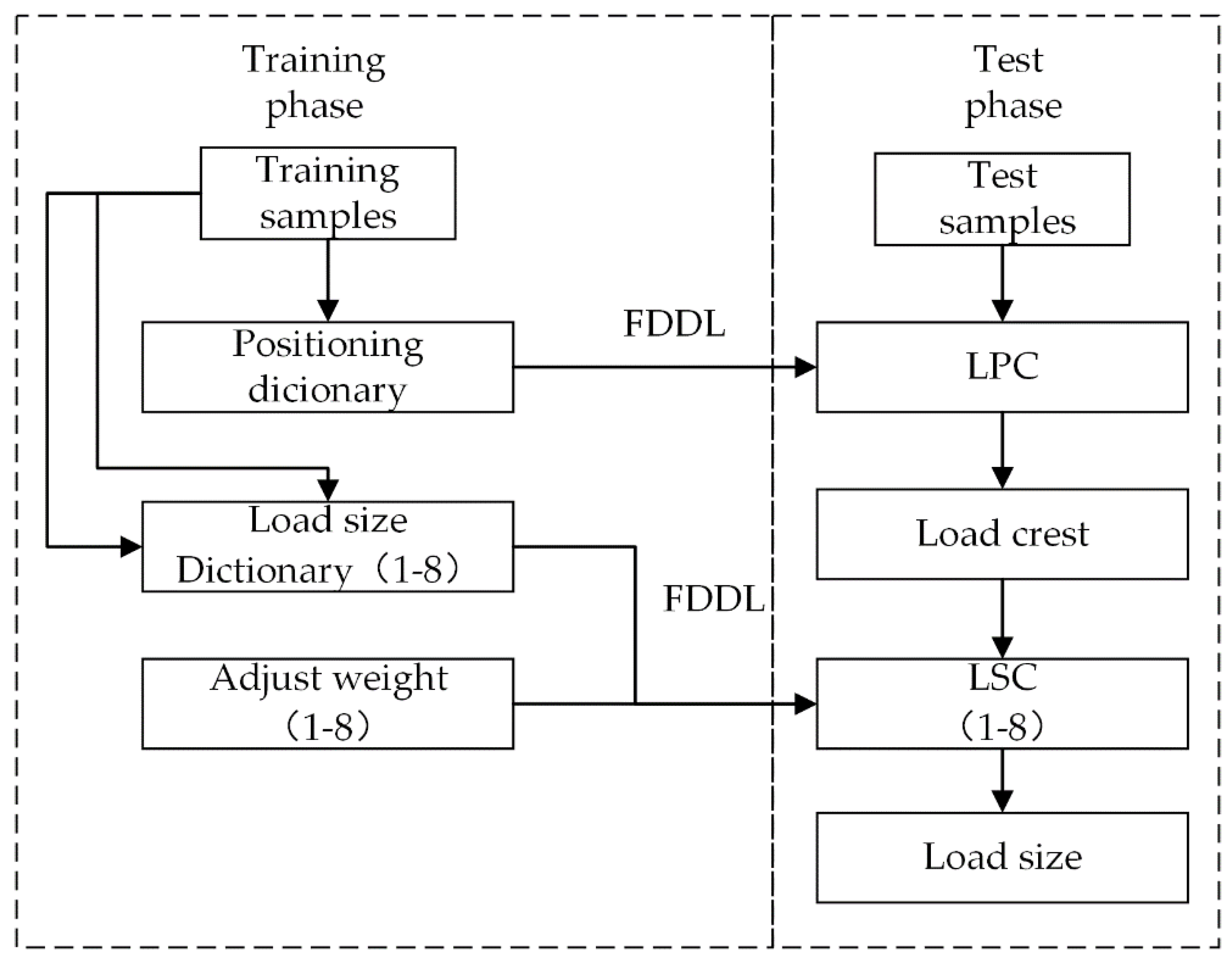
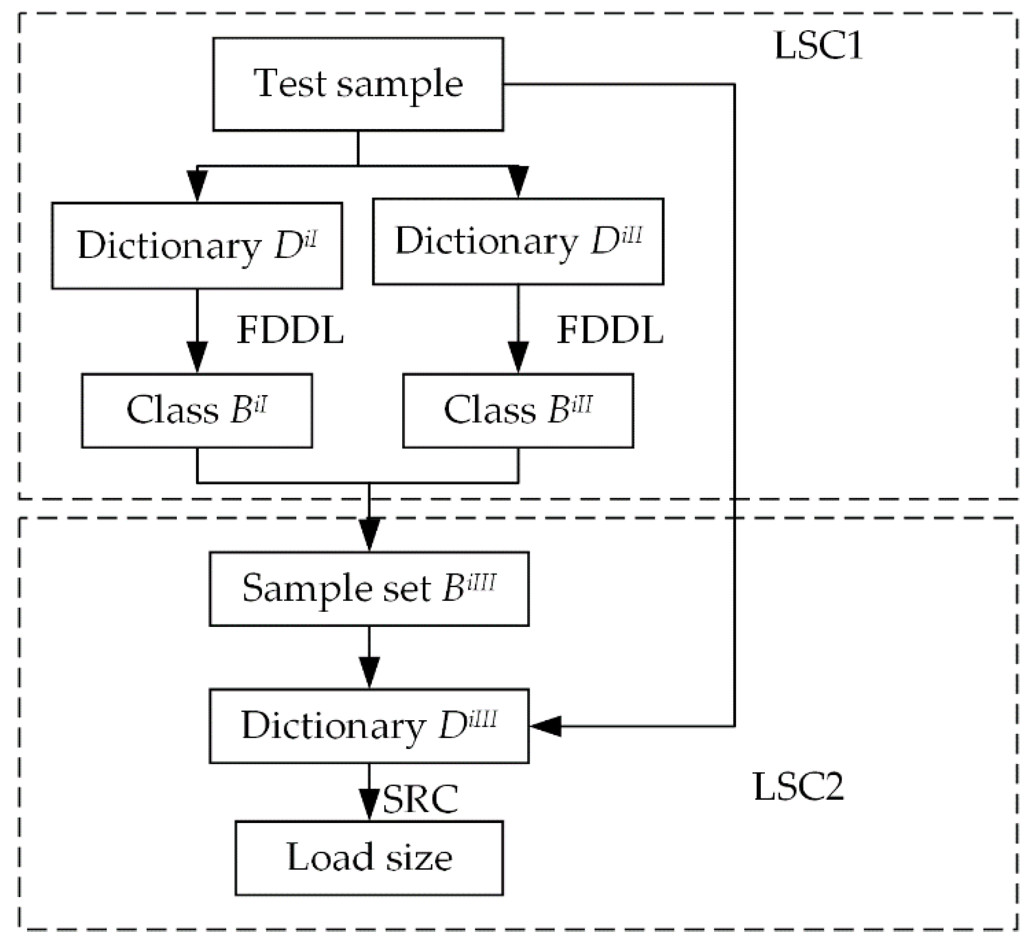
The above features must be extracted from the spectra of FBG1 and FBG2 and merged into a feature vector. The feature vector was first normalized by row and then normalized by column. The coefficient vector of the normalization of rows should be recorded; the test samples were preprocessed in the same way.

4. Algorithm Design

4.1. Algorithm Flow

To identify the load on the flexible corrugated skin, both the positions and magnitudes of the loads should be recognized. The algorithm flow for the proposed method is shown in Figure 6.
During the training phase, two types of dictionaries are learned: the positioning dictionary and the load-size dictionary. In the positioning dictionary, samples from the same crest are placed in the same group. In the load-size dictionary, each crest has a corresponding classifier for learning. In the test phase, the spectral signals first have their features extracted to obtain the test samples. The LPC is then used to identify the crest of the load, and the corresponding LSC is selected to obtain the load size.

4.2. Composition of Load-Size Dictionaries

As mentioned in Section 3.2, every sample has a corresponding load size, which can be directly regarded as an independent class, and each group contains only one sample. However, there are too many classes of samples under this dictionary composition for DL. Therefore, in the general dictionary composition, samples within a certain load range are grouped into one class, with each group containing multiple training samples.
In this study, the training samples were acquired over a fixed interval, which meant that the interval of each load-size label was the same. This led to insufficient separation between adjacent groups and a reduction in discriminative performance, as shown in Figure 6.
In Figure 7, the distance is defined as the interval of the load size. Sample k belongs to group i , and sample k + 1 belongs to group i + 1 . The distance between sample k and sample k + 1 is smaller than the distance between sample k and the center of group i . This situation is disadvantageous for the classification algorithm.
A dictionary composition of interleaved block groupings is introduced to solve the abovementioned shortcoming. In this composition, the original continuous groupings are interleaved into two sample sets, and there are sufficient distances between groups in each sample set, as shown in Figure 7.
In Figure 8, D i I is the odd blocks dictionary of the i t h crest, and D i I I the even blocks dictionary of the i t h crest. With the data collected and the samples generated according to the description in Section 3, dictionaries D 3 I and D 3 I I are chosen to demonstrate the effect of the present dictionary composition. A total of 400 training samples are obtained and divided into 40 groups, with each group containing 10 samples. The Euclidean distance between the classification centers of two adjacent classes is defined as distance   a , and the minimum Euclidean distance between samples belonging to two adjacent classes is defined as distance   c . The performance of the proposed approach for both distance   a and distance   c is shown in Figure 9.
Figure 9 illustrates that, when using interleaved block grouping, distance   c and distance   a are much larger than when using continuous block grouping. This means that when the dictionary is initiated, the discrimination of the dictionary is greatly improved.

4.3. Two-Resolution LSCs

To ensure the representation performance of DL, a certain number of atoms in the same group are required. This is the same as the number of samples in a class. Within a certain range, the expression ability and discriminative performance of the dictionary increase with the number of atoms in the sample group. The large sample groups in the LSC, however, cause the classification to have low resolution. It is difficult to achieve satisfactory resolution and discriminative performance at the same time.
In the proposed method, the two-resolution LSC shown in Figure 10 is introduced. LSC1 is a typical DL classifier with multiple atoms in a class, and LSC 2 is a local classifier generated from the results of LSC1.
In LSC2, the samples corresponding to a specific load are grouped into a single class, and the number of atoms in a class is the number of times that training samples are collected, which were included in this study. LSC1 ensures sufficient discriminative performance, and LSC2 ensures sufficient classification resolution. Ideally, the results of LSC1 ( D i I ) and LSC2 ( D i I I ) produce two adjacent classes C l a s s i I and C l a s s i I I , and then D i I I I is constructed from the atoms of C l a s s i I and C l a s s i I I . Sometimes, however, C l a s s i I and C l a s s i I I are not adjacent, and D i I I I is built by the atoms in and between these two classes. As the results from LSC1 are uncertain before the test phase, an SR classifier (SRC) that does not require DL is chosen for LSC2.

4.4. SRC Algorithm

The SRC uses a classification algorithm without DL, which makes it suitable for LSC2 [36]. In the SRC, test sample y can be linearly represented by an overcomplete dictionary A = [ A 1 , , A i , , A c ] , where A i is the sub-dictionary of class i , which is also the matrix of training samples without DL. If the code y of A satisfies l 1 -norm minimization, the following equation can be written:
a = argmin a y A a 2 2 + λ a 1 .
Then, the class of y can be determined by:
c = argmin i y A i δ i ( a ) 2 2 .

4.5. Optimized FDDL Algorithm

4.5.1. FDDL Classifiers

FDDL is a DL algorithm focused on improving the discrimination of the dictionary by introducing Fisher discrimination. The DL model of FDDL is described in Appendix A. There are two FDDL classification schemes, GC mode and LC mode. In the GC mode, the dictionary represents the test sample as a whole. This mode is suitable for situations in which the number of training samples for each class is relatively small. The solution for the GC mode is described as:
x ^ = argmin x { y D x 2 2 + γ x 1 } ,
where y is the test sample and x ^ = [ x ^ 1 , x ^ 2 , , x ^ c ] contains the coding coefficients of sub-dictionary D i . The class of y can be obtained by solving the following equation:
i d e n t i t y ( y ) = arg min i { y D i x ^ i 2 2 + ω x ^ m i 2 2 } ,
where y D i x ^ i 2 2 is the reconstruction error of D i , x ^ m i 2 2 is the distance between the coefficient vector x ^ and the mean coefficient vector m i learned for class i , and ω is the weight balancing the two terms. The GC mode is selected for the LSC.
The LC mode is designed for situations in which the dictionary is big enough to represent and classify the test samples. The solution for the LC mode is written as:
x ^ = arg min x { y D i x 2 2 + γ 1 x 1 + γ 2 x m i i 2 2 } ,
where γ 1 and γ 2 are weights for balancing the three terms and m i i is the sub-coefficient vector associated with D i . The class of y can be obtained by solving the following equation:
i d e n t i t y ( y ) = arg min i { y D i x ^ 2 2 + γ 1 x ^ 1 + γ 2 x ^ m i i 2 2 } .

4.5.2. GC Optimization

Several LSCs were designed for load-size identification. Figure 4 shows that the sensitivities of FBG1 and FBG2 are different when the load is applied on different crests. If the effects of sensor sensitivity on the LSC are considered, adjusting the contributions of different sensors for different LSCs will further improve the effect of the classification method.
The samples for the LSCs combine the features of FBG1 and FBG2. Define a sample as y = [ y 1 y 2 ] , where y 1 and y 2 are the features of FBG1 and FBG2, respectively, and define the dictionary as D = [ D 1 D 2 ] . An adjustable weight α   ( 0 α 1 ) is introduced. For the LSCs of crests 1–4, the following equation is obtained:
y α = [ y 1 y 2 α ] , D α = [ D 1 D 2 α ] .
For the LSCs of crests 5–8, the following equation is obtained:
y α = [ y 1 α y 2 ] , D α = [ D 1 α D 2 ] .
The sample and dictionary are then normalized as:
y α = y α y α 2 ,
D i α = { d i 1 a , d i 2 a , , d i k a } = { d i 1 a d i 1 a 2 , , d i j a d i j a 2 , , d i k a d i k a 2 } ,
where d i j are the atoms of D i . Using the adjustable weight, Equations (11) and (12) become:
x ^ = argmin x { y α D i α x 2 2 + γ x 1 } ,
i d e n t i t y ( y ) = arg min i { y α D i α x ^ 2 2 + ω x ^ m i 2 2 } .
In the optimization of an adjustable weight,   α is initialized to 0, Δ α (which is set as 0.05 in this paper) is the increase of α , and 1 is the end of iteration. Classification error and reconstruction error are chosen to obtain the best adjustable weight for each LSC. Classification error e r r o r c ( α )  of α is defined as:
e r r o r c ( α ) = y v Y v c y v i d e n t i t y ( y v ) 1 s i z e ( Y v ) ,
where Y v is the validation sample set and c l a s s v is the load-size label of sample v . Then, the best adjustable weight α is described as:
α = argmin α [ e r r o r c ( α ) ] , 0 α 1 .
Sometimes α is not unique. At this time, the adjustable weight α corresponding the minimum reconstruction error e r r o r r e ( α ) is the best adjustable weight:
e r r o r r e ( α ) = y v Y v y α D c α x ^ 2 2 s i z e ( Y v ) ,
α = argmin α [ e r r o r r e ( α ) ] ,
where D c is the sub-dictionary of the sample’s class. The result of Equation (24) is the adjustable weight associated with the best classification ability and represents the ability of the dictionary.

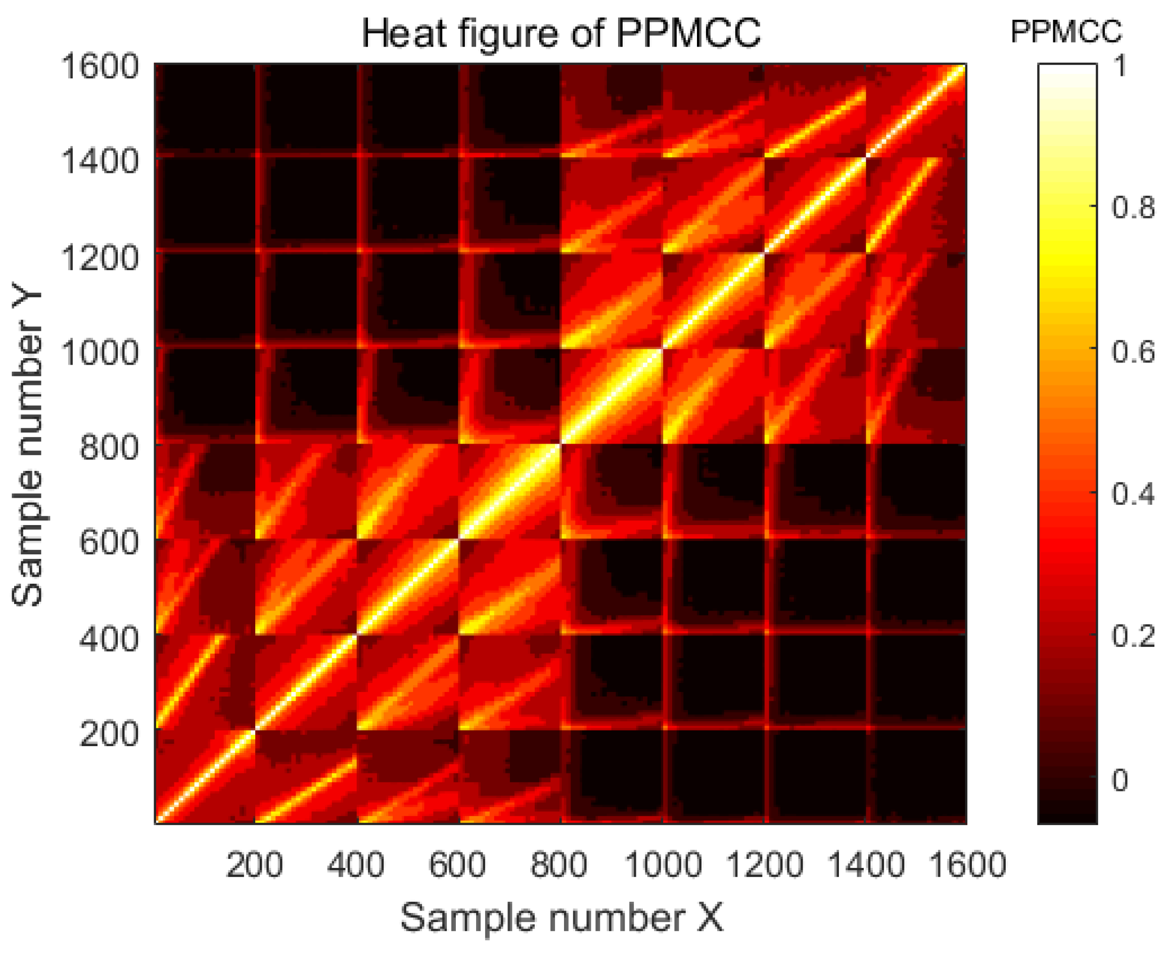
5. Experiments and Results

5.1. Parameter Selection

We collected 3200 training samples from the 8 crests. Twenty test samples associated with each crest were randomly selected, giving a total of 160 test samples.
All the parameters of FDDL were obtained following five-fold cross-validation. In the load-positioning stage, there were eight classes of the LPC, and the parameters of the FDDL were λ 1 = γ 1 = 0.1 and λ 2 = γ 2 = 0.005 . In the load-size-identification stage, there were 400 samples in each LSC1, with λ 1 = 0.05 , λ 2 = 0.01 , γ = 0.01 , and w = 0.01 . In LSC1, the range of each group was 0.5 N and there were 10 samples in each class. In LSC2, sets of dictionaries were selected with 20 atoms as a validation sample set, and λ 1 is 0.005 in the SRC. The adjustable weights of all crests (Table 3) were obtained using the algorithm in Figure 10 after the upper parameters of the LSC were determined.

5.2. Control-Group (CG) Settings

Considering the sample set, the groups of classes and identification target were different for the LPC and the LSC. To better illustrate the performance of the proposed load-identification method, the LPC and LSC results will be compared separately to that of CGs.
In the experimental group (EG), the FDDL used DL and the LPC, with the FDDL having adjustable weights chosen as DL and the LSC1 and the SRC having adjustable weights chosen as the LSC2. The samples in LSC1 were grouped with interleaved blocks, and the sample set for LSC2 was obtained from the results of LSC1.

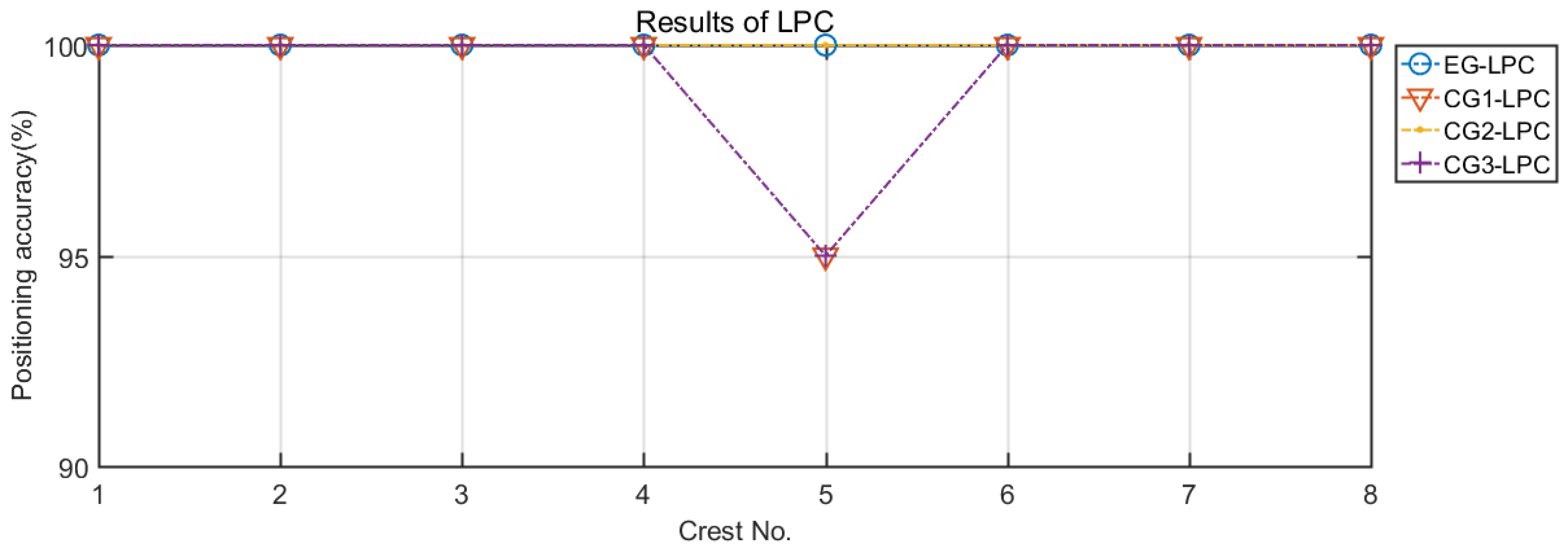
5.2.1. CG Settings of the LPCs

Three LPC CGs were used in the experiments: (i) CG1-LPC with discriminative K-mean singular value decomposition (D-KSVD) selected as the DL algorithm; (ii) CG2-LPC with label-consistent K-SVD (LC-KSVD) selected as the DL algorithm; and (iii) CG3-LPC with support vector machine (SVM) used to classify the test samples [37,38,39].

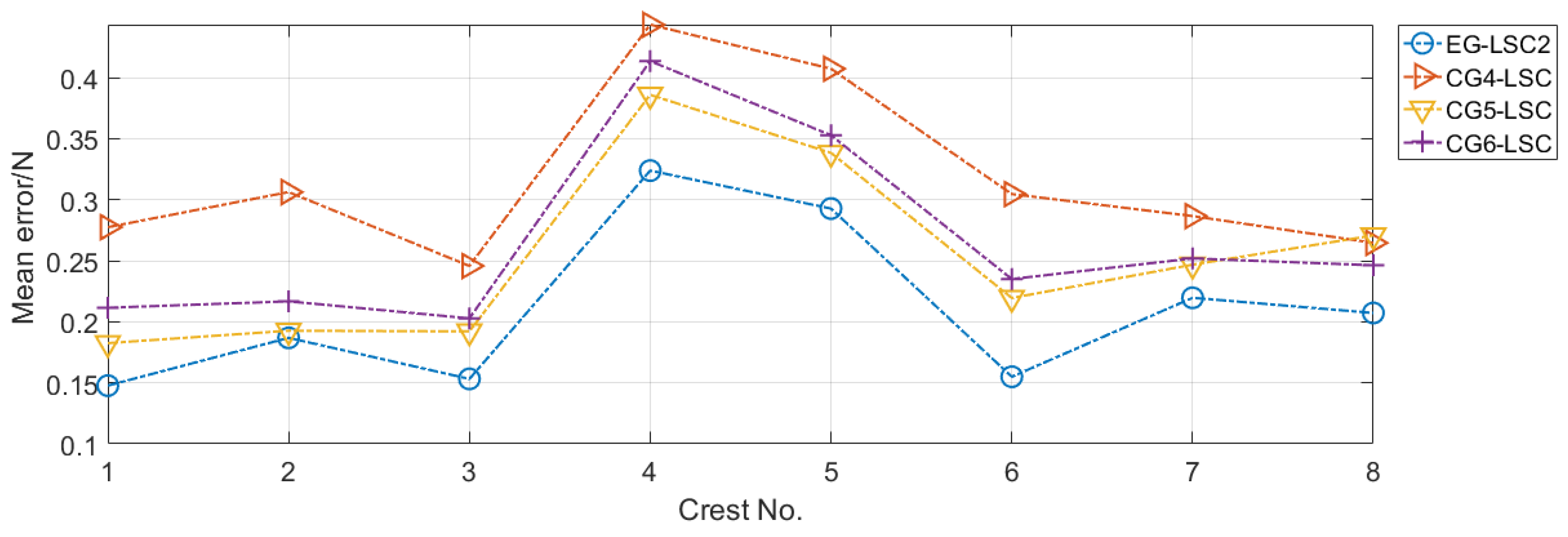
5.2.2. CG Settings of the LSCs

Six LSC CGs were used in the experiments, with the assumption that all samples were positioned correctly by the LPC.
  • CG1-LSC, with D-KSVD selected as the DL algorithm and the LSC1 classifier; LSC2 is not executed, and the other parts are the same as in EG-LSC1.
  • CG2-LSC, with LC-KSVD selected as the DL algorithm and the LSC1 classifier; LSC2 is not executed, and the other parts are the same as in EG-LSC1.
  • CG3-LSC, with the FDDL with adjustable weights selected as the DL algorithm. LSC2 is not executed, and the other parts are the same as in EG-LSC.
  • CG4-LSC, with SVM selected as LSC1 and LSC2; the other parts are the same as in EG-LSC.
  • CG5-LSC, with training samples grouped into continuous blocks in LSC1; other parts are the same as in EG-LSC. FDDL and SRC with adjustable weights are used in LSC1 and LSC2.
  • CG6-LSC, with no adjustable weights used in LSC1 and LSC2; other parts are the same as in EG-LSC.
As the results of LSC1 are uncertain before the test phase, SRC is the better choice for LSC2, as it does not need to be trained. LSC2 is not executed in CG1-LSC and CG2-LSC. A comparison of the LSC1 results from CG1-LSC, CG2-LSC, and CG3-LSC will clarify the performance of the LSC1 method presented in this research. The LSC1 results from CG6-LSC are also selected to show the improvement to FDDL from using adjustable weights.
The LSC2 results from CG4-LSC, CG5-LSC, and CG6-LSC are also compared. In CG5-LSC, the dictionary composition of LSC2 is different from that of the EG, allowing us to evaluate the effect of interleaved block groupings. CG6-LSC demonstrates the improvement of using adjustable weights.

5.3. Results and Analysis

The positioning accuracy is defined as:
R c = i = 1 , y i Y c k c i d e n t i t y L P C ( y i ) = = c k c , c { 1 , 2 , , 8 } ,
where y i is the test sample belonging to sample set Y c , c is the crest number, and k c is the number of samples from each crest. The positioning results of LPC are shown in Figure 11.
It can be seen from Figure 11 that, in the load-position-identification stage, all 160 samples are correctly identified by EG-LPC (FDDL) and CG2-LPC (LC-KSVD), while in CG1-LPC (D-KSVD) and CG3 (SVM), there are identification errors at position 5. The LPC results show that the method in this paper can accurately realize the function of load positioning.
The positioning mean error of LSC1 is defined as:
R l c = i = 1 , y i Y C k c i d e n t i t y L S C 1 ( y i ) l c ( y i ) 1 k c ,
where l c ( y i ) is the load-size label of test sample y i . In EG-LSC1, i d e n t i t y L S C 1 ( y i ) l c ( y i ) is calculated separately for odd and even dictionaries, and the smaller distance is selected as the mean error. The results for LSC1 are shown in Figure 12.
It can be seen from Figure 11 that EG-LSC obtains the best load-size-identification result. Compared with CG1 (D-KSVD), CG2 (LC-KSVD), and CG3 (SVM), the results for CG6 (FDDL) are competitive. The errors of these methods are listed in Table 4.
Compared with CG6-LSC, EG-LSC has a smaller mean error. This shows the improvement in performance that can be achieved by using adjustable weights.
The positioning mean error of LSC2 is defined as:
R l = i = 1 , y i Y C k c i d e n t i t y L S C 2 ( y i ) l ( y i ) k c ,
where l ( y i ) is the actual load size of test sample y i . The LSC2 results are shown in Figure 13. Note that the mean errors of LSC1 and LSC2 are not comparable, because l ( y i ) and l c ( y i ) have different resolutions. The LSC2 results are the final load-identification results, which are shown in Figure 13; the mean errors are summarized in Table 5.
The proposed method exhibits better performance than the other CGs, and the smallest mean error for each crest is given by EG-LSC. The result of CG4-LSC using SVM is worse than those of the other groups. The load-size-identification results at both ends are better than the data in the middle, because the second and third crests are close to FBG1 and the sixth and seventh crests are close to FBG2. The FBGs are more sensitive to the loads on these crests. The first and eighth crests are close to the fixed positions, and for a given load, the first and eighth crests display a bigger change in the strain field than the fourth and fifth crests.

6. Conclusions

This paper has proposed a load-identification method for flexible corrugated skins using an improved FDDL algorithm. All the positions were classified correctly by the proposed method, and the mean error of the proposed method is 0.2106N. Both the position and size of the load on eight crests can be identified with two FBGs. The recognition model has been optimized in several respects: (i) an interleaved block grouping has been introduced to increase the discrimination of the dictionary; (ii) a two-resolution classifier was designed for load-size classification, thus enhancing the DL effect and the class label resolution; (iii) adjustable weights were introduced to FDDL and SRC to optimize the contributions of the FBG sensors in different LSCs. The results showed that, compared with other algorithms and the original FDDL, the method proposed in this paper achieves better load-identification performance. By fully utilizing the spectral features through machine learning, this method could monitor multiple crests with few FBGs, expanding the use of SHM to the flexible skins of morphing wings.
Under the following premise, the method in this paper can also be applied to other measurement targets and environments:
(1) The features of spectra should be obvious (broadening of peak, generation of side lobes, etc.), which often means a relatively large strain and a relatively large strain gradient. On corrugated skins, the centers of the crests are the positions where the strain gradients are the large. Therefore, on other skin or plate structure, the sensors need to be pasted at the positions with a large strain and a strain gradient.
(2) The features of spectra should be discriminative, which means the spectra generated by loads of different sizes at different locations need to be different. This condition is satisfied on corrugated skins, when the deformation only occurs on chord direction as described in Figure 5, while the other structures need to be discussed and verified separately.
This paper has focused on the sparse representation model of load processing and analyzed the structure of the target specimen to optimize the algorithm. The mechanical properties of the corrugated skins have not been analyzed, so the sensor arrangement and classification algorithm could be further improved. The applicability of the proposed model to other specimens of the same specification has not yet been verified. These aspects will be considered in the next stage of research.

Author Contributions

Conceptualization, Z.Z.; methodology, Z.Z. and J.L.; software, Z.Z.; validation, J.L. and D.L.; formal analysis, Z.Z.; investigation, Z.Z.; resources, J.L. and D.L.; data curation, Z.Z.; writing of the original draft preparation, Z.Z.; writing of review and editing, Z.Z. and J.L.; visualization, Z.Z.; supervision, J.L. and D.L.; project administration, J.L.; funding acquisition, J.L. All authors have read and agreed to the published version of the manuscript.

Funding

This research was funded by the National Science Foundation of China (NSFC) (grant numbers 51405223 and U1933202). This research was also funded by the Open Funds for Key Laboratory of Civil Aircraft Health Monitoring and Intelligent Maintenance of China (grant number: NJ201812).

Institutional Review Board Statement

Not applicable.

Informed Consent Statement

Not applicable.

Data Availability Statement

Not applicable.

Conflicts of Interest

The authors declare no conflict of interest.

Appendix A

A typical DL model is described as:
J ( D , X ) = arg min ( D , X ) { A D X F 2 + λ X p + f ( X , D ) } ,
where A is the training sample, D is the sparse dictionary, and X is the coding coefficient matrix. The DL model of FDDL is written as:
J ( D , X ) = arg min ( D , X ) { i = 1 c r ( A i , D , X i ) + λ 1 X 1 + λ 2 ( t r ( S w ( X ) S B ( X ) + η X F 2 ) ) } ,
where A D X i = D 1 X i 1 + D 2 X i 2 + D c X i c , and X i = { x j } j = i denotes the coding coefficient i for set signal A i . R ( Y i , D , X i ) is the discriminative fidelity term of the atoms:
R ( A i , D , X i ) = A i D X i F 2 + A i D i X i i F 2 + j = 1 c D i X i j F 2 ,   j i .
The term λ 1 X 1 ensures the sparsity of DL, while λ 2 ( t r ( S w ( X ) S B ( X ) + η X F 2 ) ) is the discriminative fidelity term of the coding coefficient matrix, where
S W ( X ) = i = 1 c k = 1 n i ( x k ( i ) μ i ) ( x k ( i ) μ i ) T ,
S B ( X ) = i = 1 c n i ( μ i μ ) ( μ i μ ) T ,  
where μ i and μ are the centers of X i and X , respectively, and n i is the number of samples in each classification set. The optimization goal for S w ( X ) and S b ( X ) uses an adjustable relaxation η X F 2 .

References

  1. Golzar, M.; Ghabezi, P. Corrugated composite skins. Mech. Compos. Mater. 2014, 50, 137–148. [Google Scholar] [CrossRef]
  2. Thill, C.; Downsborough, J.D.; Lai, S.J.; Bond, I.P.; Jones, D.P. Aerodynamic study of corrugated skins for morphing wing applications. Aeronaut. J. 2010, 114, 237–244. [Google Scholar] [CrossRef]
  3. Thill, C.; Ethche, J.A.; Bond, I.P.; Potter, K.D.; Weaver, P.M. Composite corrugated structures for morphing wing skin applications. Smart Mater. Struct. 2010, 19, 124009. [Google Scholar] [CrossRef]
  4. Mayes, J.S.; Andrew, C.H. Composite laminate failure analysis using multicontinuum theory. Compos. Sci. Technol. 2004, 64, 379–394. [Google Scholar] [CrossRef]
  5. Maimi, P.; Mayugo, J.A.; Camanho, P.P. A three-dimensional damage model for transversely isotropic composite laminates. J. Compos. Mater. 2008, 42, 2717–2745. [Google Scholar] [CrossRef]
  6. Qiao, P.; Lestari, W.; Shah, M.; Wang, J. Dynamics-based damage detection of composite laminated beams using contact and noncontact measurement systems. J. Compos. Mater. 2007, 41, 1217–1252. [Google Scholar] [CrossRef]
  7. Brown, S. Mechanically relevant consequences of the composite laminate-like design of the abdominal wall muscles and connective tissues. Med. Eng. Phys. 2012, 34, 521–523. [Google Scholar] [CrossRef]
  8. Xin, C.; Gu, Y.; Li, M.; Li, Y.; Zhang, Z. Online monitoring and analysis of resin pressure inside composite laminate during zero-bleeding autoclave process. Polym. Compos. 2011, 32, 314–323. [Google Scholar] [CrossRef]
  9. Navaratne, R.; Dayyani, I.; Woods, B.; Friswell, M. Development and testing of a corrugated skin for a camber morphing aerofoil. In Proceedings of the 23rd AIAA/AHS Adaptive Structures Conference, Kissimmee, FL, USA, 5–9 January 2015. [Google Scholar] [CrossRef]
  10. Grenestedt, J.; Jack, R. Wrinkling of corrugated skin sandwich panels. Compos. Part A Appl. Sci. Manuf. 2007, 38, 576–589. [Google Scholar] [CrossRef]
  11. Ghabezi, P.; Golzar, M. Mechanical analysis of trapezoidal corrugated composite skins. Appl. Compos. Mater. 2013, 20, 341–353. [Google Scholar] [CrossRef]
  12. Yokozeki, T.; Aya, S.; Yoshiyasu, H. Development of variable camber morphing airfoil using corrugated structure. J. Aircr. 2014, 51, 1023–1029. [Google Scholar] [CrossRef] [Green Version]
  13. Previtali, F.; Molinari, G.; Arrieta, A.; Guillaume, M.; Ermanni, P. Design and experimental characterisation of a morphing wing with enhanced corrugated skin. J. Intell. Mater. Syst. Struct. 2016, 27, 278–292. [Google Scholar] [CrossRef]
  14. Brachman, R.; Elshimi, T.; Mak, A.; Moore, I. Testing and analysis of a deep-corrugated large-span box culvert prior to burial. J. Bridge Eng. 2012, 17, 81–88. [Google Scholar] [CrossRef]
  15. Manko, Z.; Beben, D. Dynamic testing of a corrugated steel arch bridge. Can. J. Civ. Eng. 2008, 35, 246–257. [Google Scholar] [CrossRef]
  16. Beben, D. Field Performance of Corrugated Steel Plate Road Culvert under Normal Live-Load Conditions. J. Perform. Constr. Facil. 2013, 27, 807–817. [Google Scholar] [CrossRef]
  17. Kinet, D.; Mégret, P.; Goossen, K.; Qiu, L.; Heider, D.; Caucheteur, C. Fiber Bragg grating sensors toward structural health monitoring in composite materials: Challenges and solutions. Sensors 2014, 14, 7394. [Google Scholar] [CrossRef]
  18. Wei, P.; Liu, J.; Dai, Z.; Li, M. Monitoring the shape of satellite wing frame using FBG sensors in high electronic noise, vacuum, and-196 C environment. IEEE Trans. Ind. Electron. 2016, 64, 691–700. [Google Scholar] [CrossRef]
  19. Ramzyzan, R.; Kuntjoro, W.; Rahman, M. Using embedded fiber Bragg grating (FBG) sensors in smart aircraft structure materials. Procedia Eng. 2012, 41, 600–606. [Google Scholar] [CrossRef] [Green Version]
  20. Rajabzadeh, A.; Heusdens, R.; Hendriks, R.; Groves, R. Calculation of the mean strain of smooth non-uniform strain fields using conventional FBG sensors. J. Lightwave Technol. 2018, 36, 3716–3725. [Google Scholar] [CrossRef]
  21. Ling, H.; Lau, K.; Cheng, L.; Chow, K. Embedded fibre Bragg grating sensors for non-uniform strain sensing in composite structures. Meas. Sci. Technol. 2005, 16, 2415. [Google Scholar] [CrossRef] [Green Version]
  22. Song, C.; Shang, E.; Huang, X.; Zhang, J. Monitoring the cohesive damage of the adhesive layer in CFRP double-lapped bonding joint based on non-uniform strain profile reconstruction using dynamic particle swarm optimization algorithm. Measurement 2018, 123, 235–245. [Google Scholar] [CrossRef]
  23. Zhang, Y.; Wang, B.; Lu, J. Progressive damage monitoring of corrugated composite skins by the FBG spectral characteristics. Spectrosc. Spectr. Anal. 2014, 34, 757–761. [Google Scholar] [CrossRef]
  24. Julien, M.; Elad, M.; Sapiro, G. Sparse representation for color image restoration. IEEE Trans. Image Process. 2007, 17, 53–69. [Google Scholar] [CrossRef] [Green Version]
  25. Donoho, D. Compressed sensing. IEEE Trans. Inf. Theory 2006, 52, 1289–1306. [Google Scholar] [CrossRef]
  26. Wright, J.; Ma, Y.; Mairal, J.; Sapiro, G.; Huang, T.; Yan, S. Sparse representation for computer vision and pattern recognition. Proc. IEEE 2010, 98, 1031–1044. [Google Scholar] [CrossRef] [Green Version]
  27. Zhang, L.; Zhou, W.; Chang, P.; Liu, J.; Yan, Z.; Wang, T.; Li, F. Kernel sparse representation-based classifier. IEEE Trans. Signal Process. 2011, 60, 1684–1695. [Google Scholar] [CrossRef]
  28. Ron, R.; Bruckstein, A.; Elad, M. Dictionaries for sparse representation modeling. Proc. IEEE 2010, 98, 1045–1057. [Google Scholar] [CrossRef]
  29. Kreutz-Delgado, K.; Murray, J.; Rao, B.; Engan, K.; Lee, T.; Sejnowski, T. Dictionary learning algorithms for sparse representation. Neural Comput. 2003, 15, 349–396. [Google Scholar] [CrossRef] [PubMed] [Green Version]
  30. Zheng, Z.; Xu, Y.; Yang, J.; Li, X.L.; Zhang, D. A survey of sparse representation: Algorithms and applications. IEEE Access 2015, 3, 490–530. [Google Scholar] [CrossRef]
  31. Tan, X.; Triggs, B. Enhanced local texture feature sets for face recognition under difficult lighting conditions. IEEE Trans. Image Process. 2010, 19, 1635–1650. [Google Scholar] [CrossRef] [Green Version]
  32. Yang, M.; Zhang, L.; Feng, X.; Zhang, D. Fisher discrimination dictionary learning for sparse representation. In Proceedings of the 2011 International Conference on Computer Vision, Barcelona, Spain, 6–13 November 2011. [Google Scholar] [CrossRef] [Green Version]
  33. Yang, M.; Zhang, L.; Feng, X.; Zhang, D. Sparse representation based fisher discrimination dictionary learning for image classification. Int. J. Comput. Vis. 2014, 109, 209–232. [Google Scholar] [CrossRef]
  34. Hill, K.; Meltz, G. Fiber Bragg grating technology fundamentals and overview. J. Lightwave Technol. 1997, 15, 1263–1276. [Google Scholar] [CrossRef] [Green Version]
  35. Yamada, M.; Kyohei, S. Analysis of almost-periodic distributed feedback slab waveguides via a fundamental matrix approach. Appl. Opt. 1987, 26, 3474–3478. [Google Scholar] [CrossRef] [PubMed]
  36. Wright, J.; Yang, A.; Ganesh, A.; Sastry, S.; Ma, Y. Robust face recognition via sparse representation. IEEE Trans. Pattern Anal. Mach. Intell. 2008, 31, 210–227. [Google Scholar] [CrossRef] [PubMed] [Green Version]
  37. Zhang, Q.; Li, B. Discriminative K-SVD for dictionary learning in face recognition. In Proceedings of the 2010 IEEE Computer society Conference on Computer Vision and Pattern Recognition, San Francisco, CA, USA, 5 August 2010. [Google Scholar] [CrossRef]
  38. Jiang, Z.; Zhe, L.; Davis, L. Label consistent K-SVD: Learning a discriminative dictionary for recognition. IEEE Trans. Pattern Anal. Mach. Intell. 2013, 35, 2651–2664. [Google Scholar] [CrossRef] [PubMed]
  39. Noble, W. What is a support vector machine? Nat. Biotechnol. 2006, 24, 1565–1567. [Google Scholar] [CrossRef]
Figure 1. Corrugated composite material skin specimen: (a) the crests of the specimen; (b) the position of the pasted sensors.
Aerospace 08 00134 g001
Figure 2. Diagram of the test system.
Aerospace 08 00134 g002
Figure 3. Picture of the experimental setup.
Aerospace 08 00134 g003
Figure 4. Reflecting spectrum of loads on the second crest.
Aerospace 08 00134 g004
Figure 5. The Pearson product-moment correlation coefficient (PPMCC) heat map of fiber Brag grating (FBG) sensors.
Aerospace 08 00134 g005
Figure 6. Algorithm flow of load identification.
Aerospace 08 00134 g006
Figure 7. Shortcoming of continuous block grouping.
Aerospace 08 00134 g007
Figure 8. Dictionary composition of interleaved block groupings.
Aerospace 08 00134 g008
Figure 9. Discrimination of different dictionary compositions: (a)   distance   a for two dictionary compositions; (b)   distance   c for two dictionary compositions.
Aerospace 08 00134 g009
Figure 10. Algorithm flow for load-size classifiers LSC 1 and LSC2.
Aerospace 08 00134 g010
Figure 11. Load-position classifier results.
Aerospace 08 00134 g011
Figure 12. LSC1 results with different algorithms.
Aerospace 08 00134 g012
Figure 13. Final results of different algorithm.
Aerospace 08 00134 g013
Table 1. Geometric data of the specimen.
l 1 (mm) l 2 (mm) l 3 (mm) l 4 (mm) n 1
350257.51.26
Table 2. The properties of the composite material in this research.
E 11 (GPa) E 22 (GPa) ρ (g/mm3) C f (%) C m (%) v 12
37.085.561.78 × 10−648520.26
Table 3. Adjustable weights for each crest.
Crest No.12345678
Adjustable weight (Fisher discrimination dictionary learning, FDDL)0.400.200.450.700.850.300.150.35
Adjustable weight (sparse representation classifier, SRC)1.000.750.800.850.900.800.850.75
Table 4. Mean errors of each method.
GroupEG-LSCCG1-LSCCG2-LSCCG3-LSCCG6-LSC
Mean error (N)0.18440.36250.33130.28440.2063
Table 5. Mean errors of each method.
GroupEG-LSCCG4-LSCCG5-LSCCG6-LSC
Mean error (N)0.21060.31690.25310.2663
Publisher’s Note: MDPI stays neutral with regard to jurisdictional claims in published maps and institutional affiliations.

