Abstract
Contrail cirrus has been emphasized as the largest individual component of aircraft climate impact, yet respective assessments have been based mainly on conventional radiative forcing calculations. As demonstrated in previous research work, individual impact components can have different efficacies, i.e., their effectiveness to induce surface temperature changes may vary. Effective radiative forcing (ERF) has been proposed as a superior metric to compare individual impact contributions, as it may, to a considerable extent, include the effect of efficacy differences. Recent climate model simulations have provided a first estimate of contrail cirrus ERF, which turns out to be much smaller, by about 65%, than the conventional radiative forcing of contrail cirrus. The main reason for the reduction is that natural clouds exhibit a substantially lower radiative impact in the presence of contrail cirrus. Hence, the new result suggests a smaller role of contrail cirrus in the context of aviation climate impact (including proposed mitigation measures) than assumed so far. However, any conclusion in this respect should be drawn carefully as long as no direct simulations of the surface temperature response to contrail cirrus are available. Such simulations are needed in order to confirm the power of ERF for assessing contrail cirrus efficacy.
1. Introduction
Based on a number of radiative forcing (RF) estimates yielded over the last 10 years, contrail cirrus is often supposed to form the largest individual contribution to aviation climate impact [1,2,3,4]. However, in the last (5th) report of the IPCC [5], it has been recommended to use effective radiative forcing (ERF) as the most appropriate metric for assessing the quantitative importance of various components contributing to a combined climate forcing. This paradigm change has resulted from a gradual conceptual evolution (e.g., [6]), backed by strongly indicative climate modelling evidence: The fundamental equation linking the radiative forcing to the global mean surface temperature response (ΔTsfc) via the so-called climate sensitivity parameter (λ),
is better fulfilled with a constant, forcing-independent, λ, if the conventional RF is replaced by the ERF. The evidence that, in the conventional RF framework, certain forcing agents may exhibit a climate sensitivity parameter distinctly different from that of CO2 (λCO2) has been accounted for by introducing so-called efficacy factors (r), which quantify the specific effectiveness of different forcings to induce surface temperature changes [7]:
ΔTsfc = λ RF
ΔTsfc = r λ(CO2) RF.
Since the climate sensitivity parameter is physically related to the various radiative feedback processes caused by some climate forcing (e.g., [8,9,10,11]), it can be reasoned that forcings associated with an efficacy factor smaller (larger) than unity are associated with more negative (positive) feedbacks than the reference forcing, i.e., a CO2 increase. In the revised framework, those feedbacks that develop quasi-instantaneously, in direct response to the forcing agent (so-called “rapid adjustments”), are counted as part of the (ERF) forcing. Only the feedbacks driven by the slowly evolving surface temperature response affect the climate sensitivity.
ΔTsfc = r’ λ’(CO2) ERF.
Experience suggests that efficacy values resulting for different forcings in the ERF framework (r’) deviate much less from unity than respective r values [7,12]. Yet, exceptions have also been demonstrated [13], so each radiative forcing agent has to be investigated individually in this respect.
In previous studies [14,15], line-shaped contrails have been found to exhibit an efficacy considerably less than unity under the conventional framework (Equation (2)). Hence, respective investigations targeting the quantitatively more important contrail cirrus forcing are clearly required. An attempt to treat contrail cirrus in the ERF framework, as well as consequences arising from its results, has been provided and discussed by [16] and their work is revisited here. We use the same simulations as [16] but extend the analysis of their data. Moreover, we will discuss whether the resulting contrail cirrus ERF values can be used to provide a surrogate for the efficacy of contrail cirrus.
2. Simulation Concept and ERF Results
The classical RF of contrail cirrus can be calculated from stand-alone radiation models, if all contrail and ambient properties are known (e.g., [17]). However, in order to go beyond and determine contrail cirrus ERF as well, a climate model equipped with an adequate contrail parameterization is required. The conventional RF is usually calculated from one model simulation using the technique of radiation double calling [18,19], which enables high statistical accuracy (e.g., [20]). The uncertainty of contrail cirrus RF is largely dominated by insufficient knowledge of the input parameters entering its calculation, but also by simplifications and biases in the radiation models that are applied [4,21,22]. In the ERF framework, the statistical uncertainty problem is much more severe [20], which has hampered its application for small forcings such as contrail cirrus. In preparation of the CMIP6 exercise (Coupled Model Intercomparison Project, phase 6), the various options to determine ERF have been intercompared by [20]. They recommended, as presumably the best respective approach, ERF determination via calculating the global mean difference of top of the atmosphere radiation balance from two independent model simulations. The first run includes the perturbation (in our case: contrail cirrus or increasing CO2) and the associated rapid adjustments, while the second (reference) run omits them. Both simulations have to be conducted with fixed sea surface temperature as lower boundary, thus suppressing slow feedbacks. We note that a variant of this simulation concept is running the climate model with specified dynamics (also called “nudging”), a method that was applied to contrail cirrus by [23]. This approach is thought to yield estimates lying in between the ERF and the RF value [20,24].
Quite recently, [16] have applied the pure simulation concept recommended in [20] for the calculation of contrail cirrus ERF, building on the ECHAM5/CCMod model described in [3,25]. ECHAM5/CCMod was used previously to determine the conventional RF of contrail cirrus, yielding values near 50 and 160 mWm−2, for 2006 and 2050 aircraft inventories, respectively [3,26]. It is essential to note that [16] had to scale the contrail cirrus forcing to yield statistically significant results in their ERF simulations. Therefore, the contrail cirrus simulations used as an input flight distances from the 2050 aircraft inventory of [27], which were multiplied by factors up to 12. The scenario with 12-fold increased air traffic (hereafter referred to as ATR-12) yielded a classical RF value of 701 mWm−2 and a respective ERF value of 261 mWm−2 (Figure 1), indicating an ERF reduction in almost 65%. For optimal comparison with the reference (CO2) case, a CO2 increase yielding nearly the same amount of classical RF (693 mWm−2) was employed, which resulted in a much smaller ERF reduction in only about 10%. Further simulations reported in [16] (their Figure 1) confirmed the clearly different level of ERF reduction (with respect to RF) for the contrail cirrus and the CO2 forcing.
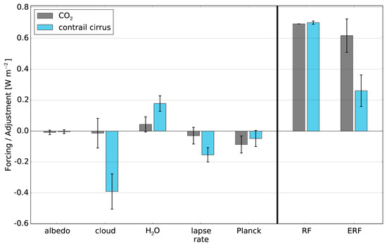
Figure 1.
Classical radiative forcing (RF), effective radiative forcing (ERF), and rapid radiative adjustments due to various physical processes (left panel), as yielded by climate model simulations using either contrail cirrus (blue) or CO2 (gray) as the forcing agent. The simulations are the same as those reported in [16]. The forcings in the simulations were scaled (see text) to ensure statistically significant ERF results. Error bars indicate confidence intervals on a 95% significance level.
A meaningful ERF estimate for the original (unscaled) aircraft inventory cannot be yielded by direct simulation, as the statistical uncertainty is then larger than the ERF value obtained as the difference between the contrail and the reference run (see [16], their Figure 1). In the next section, we will return to the question, how the validity of the findings from the scaled experiments can be ensured for the unscaled case.
3. Analysis of Rapid Radiative Adjustments
It is essential to identify and to understand the individual physical processes that control the difference between the contrail cirrus case and the CO2 case concerning the ratio of ERF and conventional RF. Otherwise there would be hardly a sound basis for comparison and validation of our results with results from other climate models, from process modelling, or from observations, especially as conventional RF is not an observable parameter. Without sufficient process understanding, the climate model results will meet considerable skepticism when to be used in assessments of overall aviation impact or of mitigation measures (e.g., [28]). However, as mentioned in the introduction, the ERF reduction can be traced to its physical origin by means of a complete analysis of feedbacks [11]. Contributions are provided by temperature changes (Planck and lapse-rate feedback), by natural cloud changes, by water vapor changes, and by snow and ice cover changes that modify the surface albedo. For details of this well-established and well-approved method, the reader is referred to respective previous studies (e.g., [11,29,30]).
This analysis approach has been applied to the rapid adjustments occurring in the contrail cirrus and CO2 simulations, as reported in [16]. Their respective results are condensed in the left part of Figure 1, where the various radiative adjustments contributing to ERF are displayed for both forcing types. Obviously, the main reason for a stronger reduction in ERF in the contrail cirrus case is a large negative radiative adjustment from natural clouds. Reference [16] provides evidence from the simulation with 12-fold air traffic scaling that the (positive, i.e., warming) radiative effect of natural cirrus gets significantly weaker in the contrail cirrus simulation. This can be explained by the physical mechanism that natural and aviation-induced ice clouds compete with each other, with respect to removing supersaturated water vapor from the ambient atmosphere through condensation to ice particles. Changes of mid-tropospheric clouds may also contribute to the negative radiative cloud adjustment (Figure 1), but their effect is less significant in the statistical sense (see [16], their Figure 5b). Rapid adjustments in the CO2 case are generally smaller (mostly statistically insignificant in Figure 1). Water vapor and lapse-rate adjustment largely compensate each other, as is usual in feedback analysis (e.g., [10,30]).
The essential factor in reducing ERF in the ATR-12 simulation is, hence, the rapid reaction of natural clouds. The tendency of reduced natural cirrus clouds near areas with maximum average contrail coverage has already been noticed by [1] in the first contrail cirrus radiative forcing estimate. However, in their study, they detected statistically significant signals only on the regional scale, using an unscaled inventory. In [16] (their Figure 5b), the natural cirrus reaction is obvious for the heavily scaled scenario, but the overall feature is also present in the less and unscaled simulations, as we show in Figure 2.
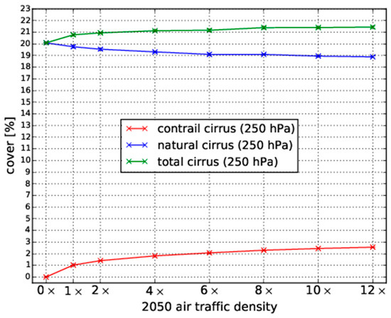
Figure 2.
Global mean coverage (in %) at 250 hPa for all (green), natural (blue), and aircraft-induced (red) cirrus clouds, derived from the contrail cirrus simulations using the 2050 aviation inventory of [27] with different scaling factors as indicated on the abscissa (same simulations as reported by [16]). Statistical uncertainties are so small that they cannot be deciphered from the graphic.
The cirrus coverage at 250 hPa is much less affected by background variability noise than the radiative parameters displayed in Figure 1. There is a decrease in natural cirrus clouds throughout the whole simulation series that compensates part of the aviation-induced (contrail) cirrus increase. Both trends develop nonlinearly with the air traffic scaling. The compensation of contrail cirrus increase by natural cirrus decrease is always substantial but varies between 32% and 46%, with a tendency to increase with the scaling. As discussed in [16] (their Figure 1), the calculated ERF reduction for contrail cirrus in the simulations with little or no scaling is getting uninterpretable due to excessive statistical noise. However, Figure 2 confirms that a crucial physical process important for the ERF reduction remains reasonably robust throughout the simulation series. This adds support to the conclusion drawn by [16], namely, that assuming an ERF reduction of similar magnitude in simulations with scaled and with realistic air traffic density is tenable, considering the uncertainty limits discussed in that paper.
4. Is the ERF/RF Ratio a Reliable Substitute for Contrail Cirrus Efficacy?
Mitigation options targeting aircraft climate impact often aim at the reduction in contrail warming at the expense of a slight increase in fuel consumption and associated CO2 emissions (e.g., [31,32,33]). To assess such measures in an optimal way, the efficacy of contrail cirrus in forcing global mean surface temperature (Equation (3)) has to be determined as exactly as possible, both with respect to the mathematical framework and the applied climate models. In this context, it is important to recognize that the conclusion of contrail cirrus ERF amounting to only 35% of the respective classical RF does not automatically imply that the contrail cirrus efficacy will be 0.35. Rather, by formulating Equations (2) and (3) for contrail cirrus (indicated by “cc” Equation (4b)) and CO2 (Equation (4a)) in both the classical and the ERF framework
it is easily realized that
ΔT(CO2)sfc = λ(CO2) RF(CO2) = λ’ (CO2) ERF(CO2)
ΔT(cc)sfc = r(cc) λ(CO2) RF(cc) = r’(cc) λ’(CO2) ERF(cc),
ERF(cc)/RF(cc) = r(cc) (ERF(CO2)/RF (CO2))/r’(cc).
Hence, the classical contrail cirrus efficacy, r(cc), only equals ERF(cc)/RF(cc), if ERF(CO2) and RF(CO2) are identical and if the contrail cirrus efficacy in the ERF framework is unity. The first condition is usually fulfilled within a 10% range (see Figure 1, or [12]). The second condition, as pointed out in the introduction, is the basic expectation and motivation when using the ERF framework, yet examples to the contrary have been demonstrated for certain forcing agents (e.g., [13,34]). Therefore, we state that contrail cirrus efficacy remains insufficiently known at the present stage, both in the classical and in the ERF framework. Direct simulations of the surface temperature response and the climate sensitivity, using a coupled atmosphere/ocean model, are necessary for this purpose.
5. Approaching the Direct Determination of Contrail Cirrus Efficacy
The atmospheric temperature signal induced by contrail cirrus in fixed sea surface temperature simulations ([16], their Figure 5d) is artificial in the sense that it is prevented from reaching an actual equilibrium response as long as the Earth’s surface does not fully interact. However, the atmospheric heating rates associated with the radiative flux anomaly induced by the contrail forcing give an impression on how strong forcing and rapid adjustments affect the atmosphere at various altitudes. Such heating rates have been calculated from the vertical profile of radiative flux change differences, both for the instantaneous and effective radiative forcing in ATR-12 (Figure 3) and for the individual rapid adjustment components (Figure 4). In the latter case, the vertical profiles of flux changes and heating rate changes result as a by-product of the PRP analysis method [11,16].
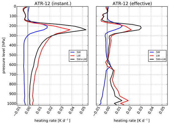
Figure 3.
Global mean atmospheric heating rates (in K d−1) induced by the contrail cirrus forcing in the ATR-12 simulation for the instantaneous forcing case (left) and for the effective forcing case (right). The latter case includes rapid atmospheric adjustments. Shortwave, longwave, and net RF are given in blue, red, and black color, respectively.
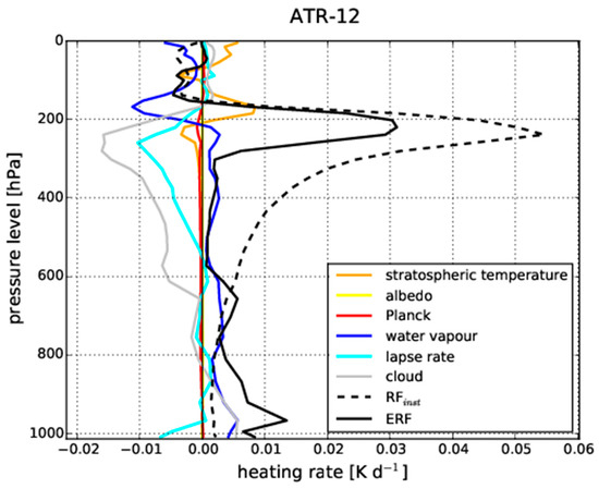
Figure 4.
Global mean atmospheric heating rates (in K d−1) induced by various rapid radiative adjustments in the ATR-12 simulations, explaining the difference between the instantaneous contrail cirrus heating rates (dashed black curve) and the effective contrail cirrus heating rates (solid black curve). The individual adjustments (colored curves) affect different atmospheric altitudes with different magnitude (see text).
Figure 3 and Figure 4 show to what extent the atmospheric radiative heating rates induced by the contrails are changing when atmospheric adjustment processes are included. The instantaneous heating rates from contrail cirrus forcing (Figure 3, left panel) resemble the vertical profile structure known from previous studies (e.g., [35,36]): a warming at the altitude of main contrail occurrence and a slight cooling above, both dominated by the longwave radiation component. Below the contrail cirrus, the atmosphere is warmed in the mean, with the negative effect due to backscattering of shortwave radiation by the contrail reducing the contrail greenhouse effect in the longwave part. If radiative adjustments are included in the ERF framework (Figure 3, right panel), atmospheric heating rates tend to decrease around the tropopause, but increase in the lower troposphere. The former effect is clearly related to the reduction in the contrail warming by decreasing adjacent natural cirrus clouds, as discussed above.
In order to understand the radiative heating rate changes over the whole tropospheric vertical profile, the components induced by the various adjustments shown in Figure 1 have also been calculated. It turns out that the lapse-rate feedback (preferred warming at higher altitudes) supports the reduced warming at contrail cirrus level, while the enhanced warming below 800 hPa is caused, with similar magnitude, by natural cloud changes and by increasing atmospheric water vapor (see Figure 4b,e in [16]). As Figure 3 and Figure 4 only show atmospheric heating rates, we add—for completeness—that the global and annual mean radiative flux changes at the Earth’s surface in ATR-12 are negative, as usual with contrail forcing (e.g., [35,37,38]). This holds for both radiative forcing frameworks, but the magnitude is reduced in the ERF case (not shown).
The complex balance of numerous effects near the Earth’s surface makes it practically impossible to predict the temperature response in the forthcoming coupled atmosphere/ocean simulations. In these simulations, the surface energy balance will be closed, including changes in sensible and latent heat exchange between atmosphere and surface (see Figure 14−6 in [6]).
6. Concluding Discussion and Outlook
We have provided further evidence that results of an ERF/RF ratio much smaller than unity, as recently reported by [16] from climate model simulations with upscaled air traffic density, do hold for realistic aviation conditions as well. If the ERF/RF factors derived by [16] and revisited here are used to convert published estimates of realistic aviation RF into ERF (and if model, parameter, and statistical uncertainties are left aside), it might be argued that contrail cirrus can no longer be regarded as the most important aviation climate impact component (Figure 5). We emphasize here, that this would be a superficial and premature conclusion.
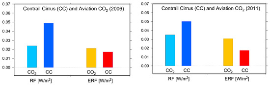
Figure 5.
Classical RF from contrail cirrus and CO2 (dark and light blue, respectively) for realistic aviation scenarios: values adopted from [4] (right box) as well as from [26] (left box). The ERF (red) counterparts have been yielded using the ERF/RF reduction factors as derived by [16]. Uncertainty bars have been deliberately omitted (but are discussed in the text).
First, the uncertainty bars for contrail cirrus RF are, in general, very large. The respective uncertainty is also far from negligible for the RF from aviation-induced CO2 increase, as discussed in [39], and once more confirmed by the most recent aviation climate impact assessment of [24]. Consider, e.g., that [4] associates his contrail cirrus RF estimate of 50 mWm−2, adopted in Figure 5 (right box), with an uncertainty range of between 20 and 150 mWm−2. This range already encloses his respective estimate of aviation-induced CO2 (35 mWm−2). At the same time, [16] associate their ERF reduction best estimate of 65% with an uncertainty range between 49% and 77%. The ERF/RF ratio of 35% has been used to derive contrail cirrus ERF from contrail cirrus RF for Figure 5, but its statistical uncertainty adds on the known physical uncertainties of RF. While it is not perfectly clear how the various uncertainty ranges are to be combined, it is obvious that contrail cirrus ERF, as calculated in this way, will have an even higher relative uncertainty than that given by [4] for the conventional contrail cirrus RF.
Second, [16] have pointed out that contrail cirrus ERF results from only one climate model need independent backing from other models, particularly because cirrus cloud feedbacks (obviously of crucial importance here) have shown large inter-model spread even in CO2 increase simulations (e.g., [9,40]). Further model studies on the subject are therefore badly needed.
Third, as pointed out above, the ERF/RF ratio does not form an exact substitute for contrail cirrus efficacy in the classical RF framework. It is necessary to determine the actual global mean surface temperature response, climate sensitivity, and efficacy of contrail cirrus by direct climate model simulations. Only these can clarify whether contrail cirrus efficacy in the ERF framework is unity, as expected from theory. This will be the next step, using the model adopted in [16] in a setup with an interactive ocean surface. However, such simulations will profit from the experience gained from the simulations of contrail cirrus ERF provided by [16], particularly with respect to the application of the air traffic density scaling. In addition, we note that it is desirable to gain deeper understanding on possible limits of the scaling method in producing results representative for the unscaled situation, especially concerning potential nonlinearities in the natural cloud feedback.
Realizing the various uncertainties, it is not surprising that the quantitative comparison of contrail cirrus ERF and aviation CO2 ERF suggested from Figure 5 (contrail cirrus ERF smaller) differs from that given in the new assessment paper by [24] (contrail cirrus ERF larger). While the ERF/RF ratio determined by [16] for contrail cirrus has been accounted for in [24], the latter study has carefully compiled all available results related to the subject, going to great length to make them as comparable as possible by including corrections of some systematic biases. The ERF multimodel best estimate of [24] also includes results yielded using the nudging concept [23]. More research is necessary to ensure the equivalence of the methods applied so far for estimating contrail cirrus ERF. This study agrees with that by [24] that a comparison in terms of ERF instead of RF brings the contrail cirrus and aviation CO2 effects closer to each other in size. Deciding the question whether contrail cirrus or aviation CO2 ERF is larger depends to a large degree on the corresponding classical RF estimates. Rather than further arguing this point, we want to conclude here that, at the present stage, both effects can be assumed to be of comparable magnitude in terms of ERF, so that neither one can be neglected when considering and assessing mitigation measures.
Author Contributions
Methodology, investigation and interpretation, M.B. and M.P.; conceptualization, project administration, and writing—original draft preparation M.P.; software, formal analysis and visualization, M.B.; supervision, M.P., U.B., and L.B.; review and editing M.B., U.B., and L.B. All authors have read and agreed to the published version of the manuscript.
Funding
This research received no external funding.
Institutional Review Board Statement
Not applicable.
Informed Consent Statement
Not applicable.
Data Availability Statement
Data from the ECHAM model simulations (which are the same as those reported in reference [16]) can be obtained from the authors on request.
Acknowledgments
High-performance supercomputing resources were used from the DKRZ, Deutsches Klimarechenzentrum, Hamburg. We thank Klaus Gierens (DLR) and several anonymous referees for their critical comments that lead to improvements of the original manuscript.
Conflicts of Interest
The authors declare no conflict of interest.
References
- Burkhardt, U.; Kärcher, B. Global radiative forcing from contrail cirrus. Nat. Clim. Change 2011, 1, 54–58. [Google Scholar] [CrossRef]
- Schumann, U.; Graf, K. Aviation induced cirrus and radiation changes at diurnal timescales. J. Geophys. Res. Atmos. 2013, 118, 2404–2421. [Google Scholar] [CrossRef]
- Bock, L.; Burkhardt, U. Reassessing properties and radiative forcing of contrail cirrus using a climate model. J. Geophys. Res. Atmos. 2016, 121, 9717–9736. [Google Scholar] [CrossRef]
- Kärcher, B. Formation and radiative forcing of contrail cirrus. Nat. Comm. 2018, 9, 1824. [Google Scholar] [CrossRef]
- Myhre, G.; Shindell, D.T.; Bréon, F.; Collins, W.; Fuglestvedt, J.S.; Huang, J.; Koch, D.; Lamarque, J.-F.; Lee, D.S.; Mendoza, B.; et al. Anthropogenic and natural radiative forcing. In Climate Change 2013: The Physical Science Basis. Contribution of Working Group I to the fifth Assessment Report of the Intergovernmental Panel on Climate Change; Stocker, T.F., Qin, D., Plattner, G.-K., Tignor, M., Allen, S.K., Boschung, J., Nauels, A., Xia, Y., Bex, V., Midgley, P.M., Eds.; Cambridge University Press: Cambridge, UK; New York, NY, USA, 2013; pp. 659–740. [Google Scholar]
- Ramaswamy, V.; Collins, W.; Haywood, J.; Lean, J.; Mahowald, N.; Myhre, G.; Naik, V.; Shine, K.P.; Soden, B.; Stenchikov, G.; et al. A century of progress in atmospheric and related sciences: Celebrating the American Meteorological Society Centennial. Meteor. Monogr. 2019, 59, 14.1–14.101. [Google Scholar] [CrossRef]
- Hansen, J.; Sato, M.; Ruedy, R.; Nazarenko, L.; Lacis, A.; Schmidt, G.A.; Russell, G.; Aleinov, I.; Bauer, M.; Bauer, S.; et al. Efficacy of climate forcings. J. Geophys. Res. 2005, 110, D18104. [Google Scholar] [CrossRef]
- Boer, M.; Yu, B. Climate sensitivity and response. Clim. Dyn. 2003, 20, 415–429. [Google Scholar] [CrossRef]
- Bony, S.; Colman, R.; Kattsov, V.M.; Allan, R.P.; Bretherton, C.S.; Dufresne, J.-L.; Hall, A.; Hallegatte, S.; Holland, M.M.; Ingram, W.; et al. How well do we understand and evaluate climate change processes? J. Clim. 2006, 19, 2445–2482. [Google Scholar] [CrossRef]
- Soden, B.J.; Held, I.M. An assessment of climate feedbacks in ocean-atmosphere models. J. Clim. 2006, 19, 3345–3360. [Google Scholar] [CrossRef]
- Rieger, V.; Dietmüller, S.; Ponater, M. Can feedback analysis be used to uncover the physical origin of climate sensitivity and efficacy differences? Clim. Dyn. 2017, 49, 2831–2844. [Google Scholar] [CrossRef]
- Richardson, T.B.; Forster, P.M.; Smith, P.J.; Maycock, A.C.; Wood, T.; Andrews, T.; Boucher, O.; Faluvegi, G.; Fläschner, D.; Hodnebrog, Ø.; et al. Efficacy of climate forcings in PDRMIP models. J. Geophys. Res. Atmos. 2019, 124, 12824–12844. [Google Scholar] [CrossRef]
- Marvel, K.; Schmidt, G.A.; Miller, R.L.; Nazarenko, E.S. Implications for climate sensitivity from the response of individual forcings. Nat. Clim. Chang. 2016, 6, 389. [Google Scholar] [CrossRef]
- Ponater, M.; Marquart, S.; Sausen, R.; Schumann, U. On contrail climate sensitivity. Geophys. Res. Lett. 2005, 32, L10706. [Google Scholar] [CrossRef]
- Rap, A.; Forster, P.M.; Haywood, J.; Jones, A.; Boucher, O. Estimating the climate effect of contrails using the UK met office climate model. Geophys. Res. Lett. 2010, 37, L20703. [Google Scholar] [CrossRef]
- Bickel, M.; Ponater, M.; Bock, L.; Burkhardt, U.; Reineke, S. Estimating the effective radiative forcing of contrail cirrus. J. Clim. 2020, 33, 1991–2005. [Google Scholar] [CrossRef]
- Schumann, U.; Mayer, B.; Graf, K.; Mannstein, H. A parametric radiative forcing model for contrail cirrus. J. Appl. Meteor. Climatol. 2012, 51, 1391–1406. [Google Scholar] [CrossRef]
- Chung, E.-S.; Soden, B.J. An assessment of methods for computing radiative forcing in climate models. Environ. Res. Lett. 2015, 10, 074004. [Google Scholar] [CrossRef]
- Dietmüller, S.; Jöckel, P.; Tost, H.; Kunze, M.; Gellhorn, C.; Brinkop, S.; Frömming, C.; Ponater, M.; Steil, B.; Lauer, A.; et al. A new radiation infrastructure for the Modular Earth Submodel System (MESSy, based on version 2.51). Geosci. Model Dev. 2016, 9, 2209–2222. [Google Scholar] [CrossRef]
- Forster, P.M.; Richardson, T.B.; Smith, P.J.; Maycock, A.C.; Samset, B.H.; Myhre, G.; Andrews, T.; Pincus, R.; Schulz, M. Recommendations for diagnosing effective radiative forcing from climate models for CMIP6. J. Geophys. Res. Atmos. 2016, 124, 12824–12844. [Google Scholar] [CrossRef]
- Myhre, G.; Kvalevåg, M.; Rädel, G.; Cook, J.; Shine, K.P.; Clark, H.; Karcher, F.; Markowicz, K.; Kardas, A.; Wolkenberg, P.; et al. Intercomparison of radiative forcing calculations of stratospheric water vapour and contrails. Meteorol. Z. 2009, 18, 585–596. [Google Scholar] [CrossRef]
- Lee, D.S.; Pitari, G.; Grewe, V.; Gierens, K.; Penner, J.L.; Petzold, A.; Prather, M.J.; Schumann, U.; Bais, A.; Berntsen, T.; et al. Transport impacts on atmosphere and climate: Aviation. Atmos. Environ. 2010, 44, 4678–4734. [Google Scholar] [CrossRef] [PubMed]
- Chen, C.; Gettelman, A. Simulated radiative forcing from contrails and contrail cirrus. Atmos. Chem. Phys. 2013, 13, 12525–12536. [Google Scholar] [CrossRef]
- Lee, D.S.; Fahey, D.W.; Skowron, A.; Allen, M.R.; Burkhardt, U.; Chen, Q.; Doherty, S.J.; Freeman, S.; Forster, P.M.; Fuglestvedt, J.S.; et al. The contribution of global aviation to anthropogenic climate forcing for 2010 to 2018. Atmos. Environ. 2021, 244, 117834. [Google Scholar] [CrossRef]
- Bock, L.; Burkhardt, U. The temporal evolution of a long-lived contrail cirrus cluster: Simulations with a global climate model. J. Geophys. Res. Atmos. 2016, 121, 3548–3565. [Google Scholar] [CrossRef]
- Bock, L.; Burkhardt, U. Contrail radiative forcing for future air traffic. Atmos. Chem. Phys. 2019, 19, 8163–8174. [Google Scholar] [CrossRef]
- Wilkerson, J.; Jacobsen, M.Z.; Malwitz, A.; Balasubramanian, S.; Wayson, R.; Fleming, G.; Naiman, A.D.; Lele, S.K. Analysis of emission data from global commercial aviation: 2004 and 2006. Atmos. Chem. Phys. 2010, 10, 6391–6408. [Google Scholar] [CrossRef]
- Fuglestvedt, J.S.; Berntsen, T.; Myhre, G.; Rypdal, K.; Bielveldt-Skeie, R. Climate forcing from the transport sectors. Proc. Nat. Acad. Sci. USA 2008, 105, 454–458. [Google Scholar] [CrossRef]
- Smith, P.J.; Kramer, R.J.; Myhre, G.; Forster, P.M.; Soden, B.J.; Andrews, T.; Boucher, O.; Faluvegi, G.; Fläschner, D.; Hodnebrog, Ø.; et al. Understanding rapid adjustments to diverse forcing agents. Geophys. Res. Lett. 2018, 45, 12023–12031. [Google Scholar] [CrossRef]
- Sherwood, S.C.; Webb, M.J.; Annan, J.D.; Arman, K.C.; Forster, P.M.; Hargreaves, J.C.; Hegerl, G.; Klein, S.A.; Marvel, K.D.; Rohling, E.J.; et al. An assessment of Earth’s climate sensitivity using multiple lines of evidence. Rev. Geophys. 2020, 58, 1–92. [Google Scholar] [CrossRef]
- Frömming, C.; Ponater, M.; Dahlmann, K.; Grewe, V.; Lee, D.; Sausen, R. Aviation induced radiative forcing and surface temperature change in dependency of emission altitude. J. Geophys. Res. Atmos. 2012, 117, D19104. [Google Scholar] [CrossRef]
- Teoh, R.; Schumann, U.; Stettler, M.E.J. Beyond contrail avoidance: Efficacy of flight altitude changes to minimise contrail climate forcing. Aerospace 2020, 7, 121. [Google Scholar] [CrossRef]
- Matthes, S.; Lührs, B.; Dahlmann, K.; Grewe, V.; Linke, F.; Yin, F.; Klingaman, E.; Shine, K.P. Climate optimized trajectories and robust mitigation potential: Flying ATM4E. Aerospace 2020, 7, 156. [Google Scholar] [CrossRef]
- Shine, K.P.; Highwood, E.J.; Rädel, G.; Stuber, N.; Balkanski, Y. Climate model simulations of the impact of aerosols from road transport and shipping. Atmos. Oceanic Opt. 2012, 25, 62–70. [Google Scholar] [CrossRef]
- Meerkötter, R.; Schumann, U.; Doelling, D.R.; Minnis, P.; Nakajima, T.; Tsushima, Y. Radiative forcing by contrails. Ann. Geophysicae Atmos. Hydro. Space Sci. 1999, 17, 1080–1097. [Google Scholar]
- Ponater, M.; Marquart, S.; Sausen, R. Contrails in a comprehensive global climate model: Parameterization and radiative forcing results. J. Geophys. Res. 2002, 107, 4164. [Google Scholar] [CrossRef]
- Dietmüller, S.; Ponater, M.; Sausen, R.; Hoinka, K.-P.; Pechtl, S. Contrails, natural clouds, and diurnal temperature range. J. Clim. 2008, 21, 5061–5075. [Google Scholar] [CrossRef]
- Schumann, U.; Mayer, B. Sensitivity of surface temperature to radiative forcing by contrail cirrus in a radiative-mixing model. Atmos. Chem. Phys. 2017, 17, 13833–13848. [Google Scholar] [CrossRef]
- Lee, D.S.; Fahey, D.W.; Forster, P.M.; Newton, P.J.; Wit, R.C.N.; Lim, L.L.; Owen, B.; Sausen, R. Aviation and global climate change in the 21st century. Atmos. Environ. 2009, 43, 3520–3537. [Google Scholar] [CrossRef]
- Zelinka, M.D.; Taylor, K.E.; Andrews, T.; Webb, M.J.; Gregory, J.M.; Forster, P.M. Contributions of different cloud types to feedbacks and rapid adjustments in CMIP5. J. Clim. 2013, 26, 5007–5027. [Google Scholar] [CrossRef]


Publisher’s Note: MDPI stays neutral with regard to jurisdictional claims in published maps and institutional affiliations. |
© 2021 by the authors. Licensee MDPI, Basel, Switzerland. This article is an open access article distributed under the terms and conditions of the Creative Commons Attribution (CC BY) license (http://creativecommons.org/licenses/by/4.0/).