
Improved Supersonic Turbulent Flow Characteristics Using Non-Linear Eddy Viscosity Relation in RANS and HPC-Enabled LES


Abstract
1. Introduction
2. Methodology
2.1. RANS Details
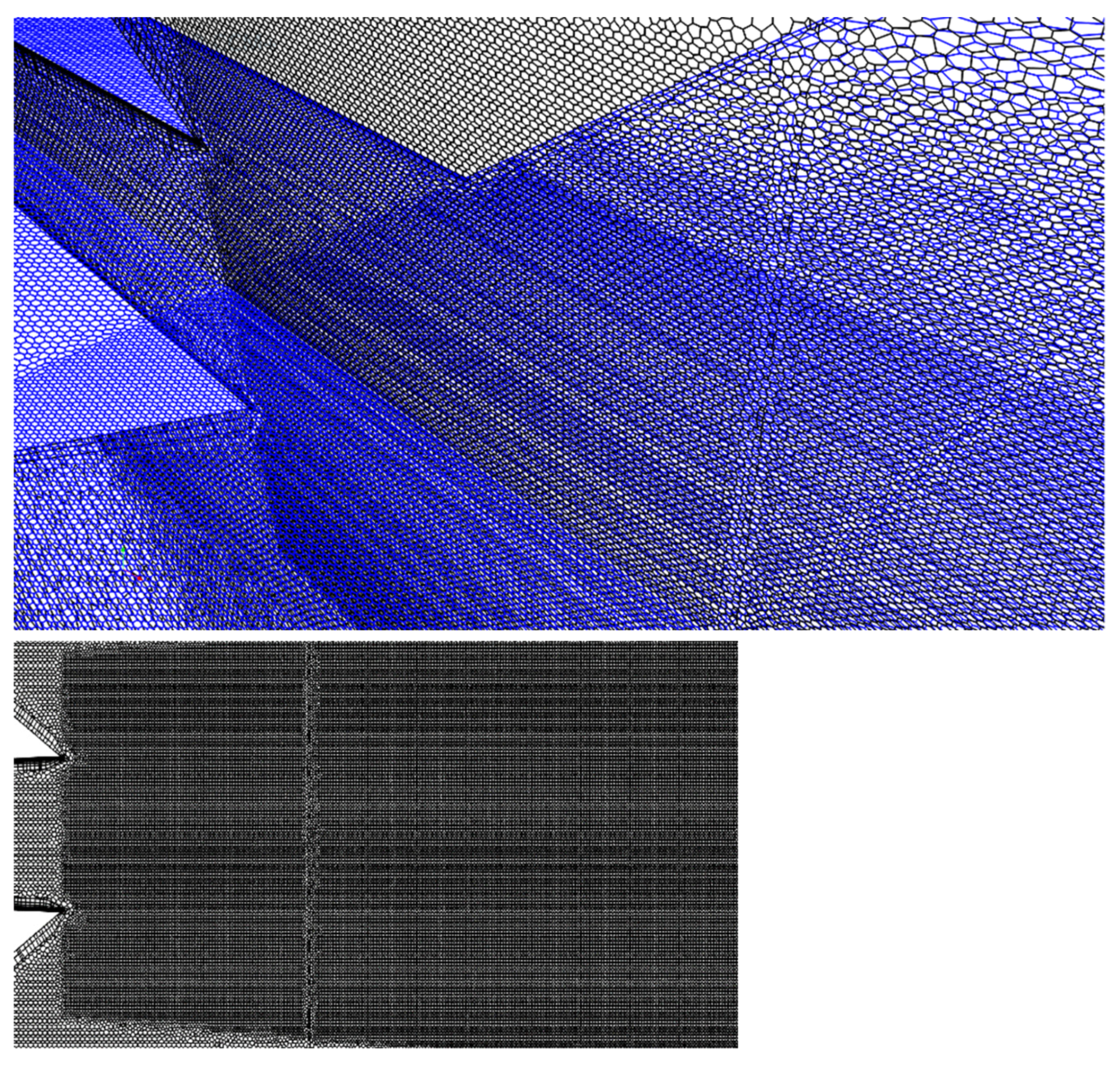
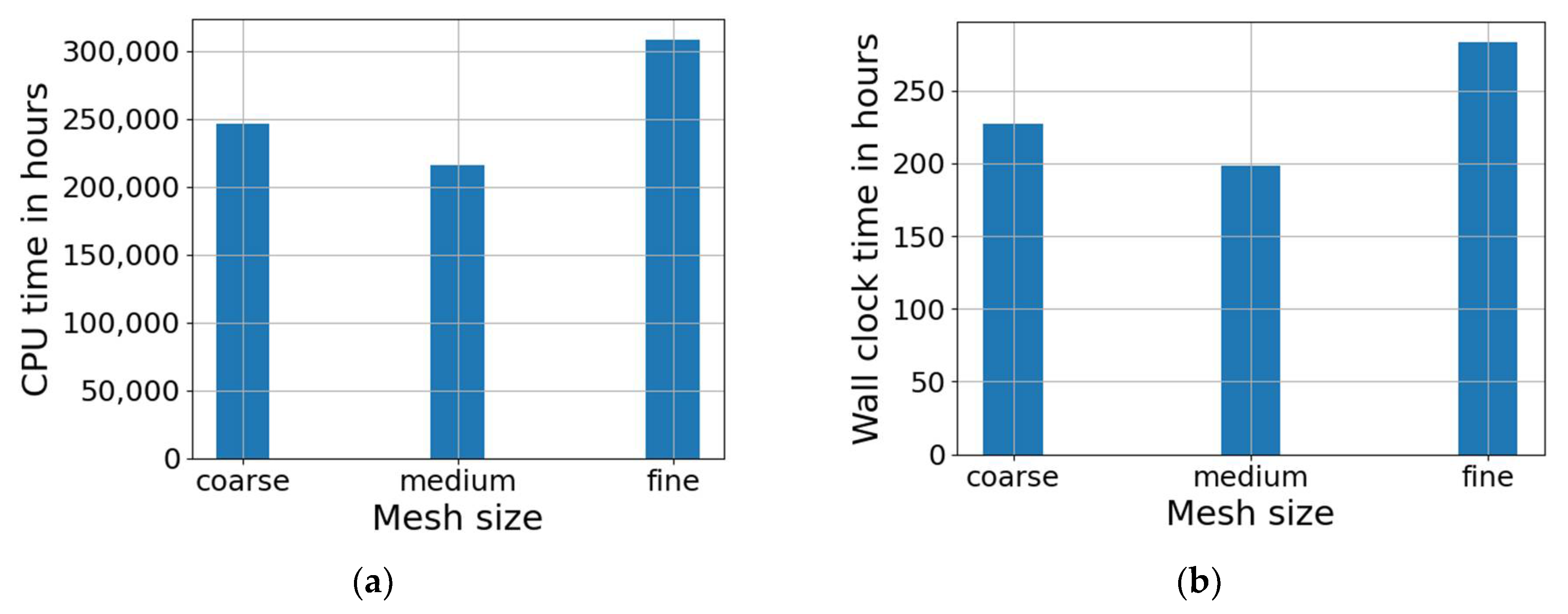
2.2. LES Details
2.3. Sensitivity of K-Omega SST with QCR towards Diffusion and Dissipation
2.4. Validation
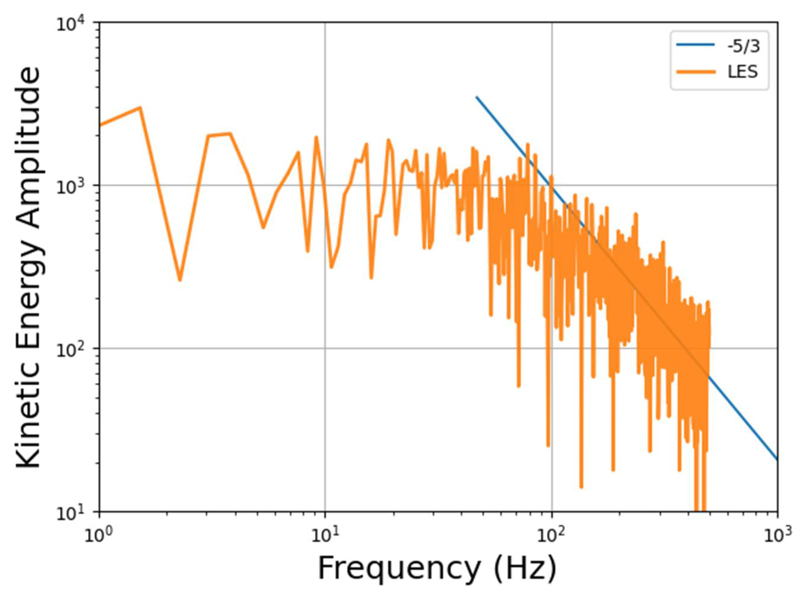
2.5. Kinetic Energy Spectrum in LES
3. Results
3.1. Turbulent Kinetic Energy
3.2. Shear Layer Profiles
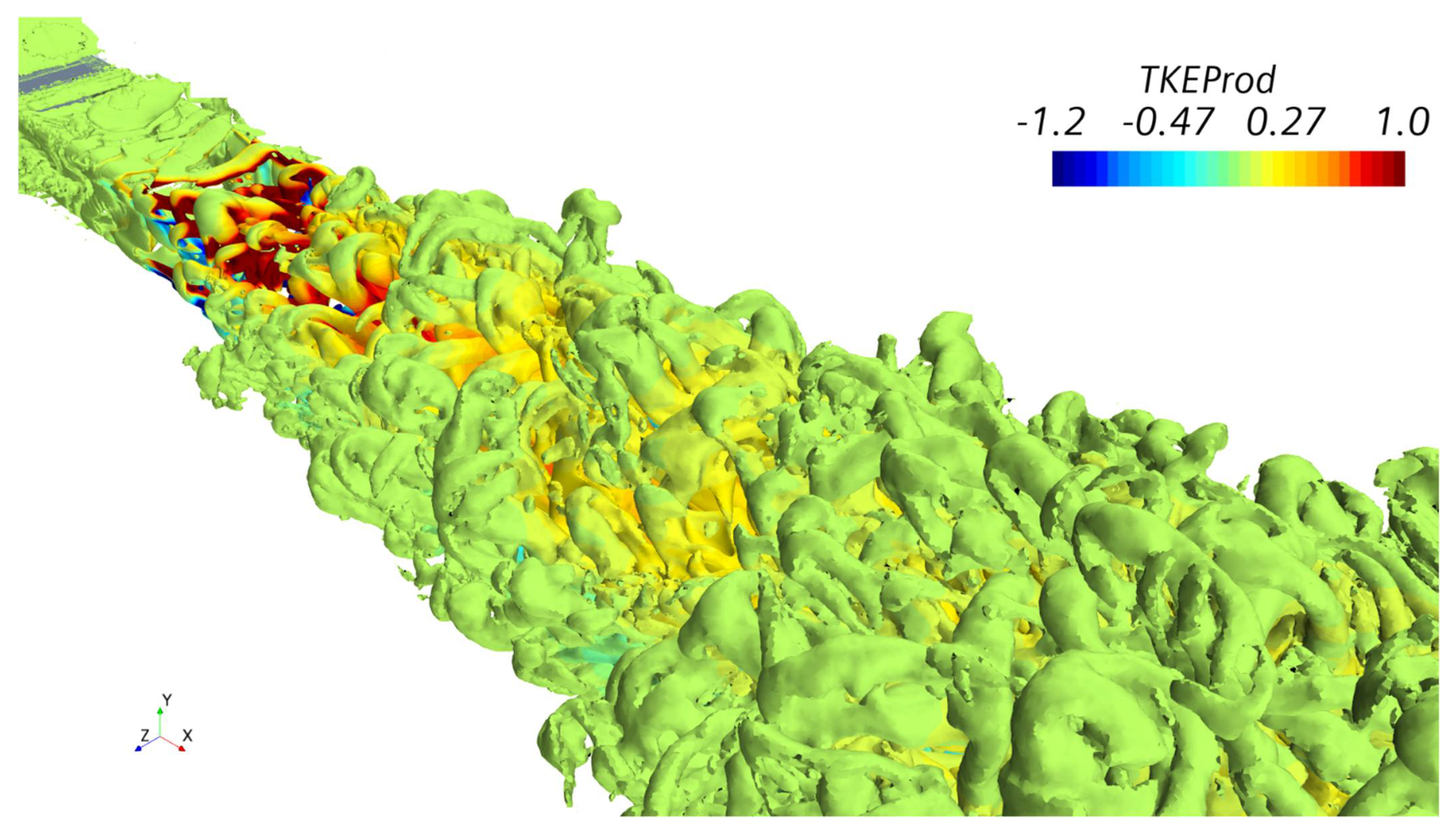
3.3. Turbulent Kinetic Energy Production and Reynolds Stresses
3.4. Retropropulsion Flow Physics—A Special Case Analysis
- Supersonic nozzle-exit Mach and subsonic freestream;
- Subsonic nozzle-exit Mach and subsonic freestream:
- (a)
- high subsonic;
- (b)
- low subsonic.
4. Conclusions
Author Contributions
Funding
Institutional Review Board Statement
Informed Consent Statement
Data Availability Statement
Acknowledgments
Conflicts of Interest
Nomenclature
| AR | Aspect Ratio |
| CFD | Computational Fluid Dynamics |
| CPU | Central processing unit |
| DNS | Direct numerical simulation |
| HPC | High performance computing |
| LES | Large Eddy Simulation |
| NPR | Nozzle pressure ratio |
| PIV | Particle image velocimetry |
| QCR | Quadratic constitutive relation |
| TKE | Turbulent Kinetic Energy |
| RANS | Reynolds Averaged Navier Stokes |
| SATA | Serial advanced technology attachment |
| SSD | Solid state drive |
| SST | Shear Stress Transport |
| WALE | Wall adapting local eddy viscosity |
| u | Axial component of velocity |
| De | Nozzle equivalent diameter |
| uj | Jet velocity at nozzle exit |
| Jet density at nozzle exit |
Appendix A
- 2× AMD EPYC 7452 CPUs (32 Cores, 2.3 GigaHertz);
- 256 GB RAM (16× 16 GigaBytes Dual Rank x8 DDR4-3200 DIMMS);
- 1× HPE 960GB SATA 6G Read Intensive SFF SSD;
- 100 gb/s InfiniBand network card.
References
- Schmitt, F.G. About Boussinesq’s turbulent viscosity hypothesis: Historical remarks and a direct evaluation of its validity. Comptes Rendus Mécanique 2007, 335, 617–627. [Google Scholar] [CrossRef]
- Sforza, P.; Steiger, M.; Trentacoste, N. Studies on three-dimensional viscous jets. AIAA J. 1966, 4, 800–806. [Google Scholar] [CrossRef]
- Sfeir, A. The velocity and temperature fields of rectangular jets. Int. J. Heat Mass Transf. 1976, 19, 1289–1297. [Google Scholar] [CrossRef]
- Koshigoe, S.; Gutmark, E.; Schadow, K.; Tubis, A. Initial development of noncircular jets leading to axis switching. AIAA J. 1989, 27, 411–419. [Google Scholar] [CrossRef]
- Sfeir, A. Investigation of Three-Dimensional Turbulent Rectangular Jets. AIAA J. 1979, 17, 1055–1060. [Google Scholar] [CrossRef]
- Zaman, K.B.M.Q. Axis switching and spreading of an asymmetric jet: The role of coherent structure dynamics. J. Fluid Mech. 1996, 316, 1–27. [Google Scholar] [CrossRef]
- Gutmark, E.; Schadow, K.C.; Bicker, C.J. Near acoustic field and shock structure of rectangular supersonic jets. AIAA J. 1990, 28, 1163–1170. [Google Scholar] [CrossRef]
- Krothapalli, A.; Baganoff, D.; Karamcheti, K. On the mixing of a rectangular jet. J. Fluid Mech. 1981, 107, 201–220. [Google Scholar] [CrossRef]
- Bobba, C.R.; Ghia, K.N. A study of three-dimensional compressible turbulent jets. In Proceedings of the 2nd Symposium on Turbulent Shear Flows; Imperial College: London, UK, 1979; pp. 1–26. [Google Scholar]
- Moin, P.; Kim, J. Tackling Turbulence with Supercomputers. Sci. Am. 1997, 276, 62–68. [Google Scholar] [CrossRef]
- Brès, G.; Jordan, P.; Jaunet, V.; Rallic, M.; Cavalieri, A.; Towne, A.; Lele, S.; Colonius, T.; Schmidt, O. Importance of the nozzle-exit boundary-layer state in subsonic turbulent jets. J. Fluid Mech. 2018, 851, 83–124. [Google Scholar] [CrossRef]
- Bogey, C.; Bailly, C. Turbulence and energy budget in a self-preserving round jet: Direct evaluation using large eddy simulation. J. Fluid Mech. 2009, 627, 129–160. [Google Scholar] [CrossRef]
- Viswanath, K.; Johnson, R.; Corrigan, A.; Kailasanath, K.; Mora, P.; Baier, F.; Gutmark, E. Noise Characteristics of a Rectangular vs. Circular Nozzle for Ideally Expanded Jet Flow. In Proceedings of the 54th AIAA Aerospace Sciences Meeting, San Diego, CA, USA, 4–8 January 2016. [Google Scholar]
- Bellan, J. Large-Eddy Simulation of Supersonic Round Jets: Effects of Reynolds and Mach Numbers. AIAA J. 2016, 54, 1482–1498. [Google Scholar] [CrossRef]
- Baier, F.; Mora, P.; Gutmark, E.; Kailasanath, K. Flow measurements from a supersonic rectangular nozzle exhausting over a flat surface. In Proceedings of the 55th AIAA Aerospace Sciences Meeting, Grapevine, TX, USA, 9–13 January 2017; p. 932. [Google Scholar]
- Baier, F.; Karnam, A.; Gutmark, E. Cold flow measurements of supersonic low aspect ratio jet-surface interactions. Flow Turbul. Combust. 2019, 105, 1–30. [Google Scholar] [CrossRef]
- Bridges, J.; Wernet, M. Turbulence Measurements of Rectangular Nozzles with Bevel. In Proceedings of the 53rd AIAA Aerospace Sciences Meeting, Kissimmee, FL, USA, 5–9 January 2015. [Google Scholar]
- Bhide, K.; Siddappaji, K.; Abdallah, S. A combined effect of wall curvature and aspect ratio on the performance of rectangular supersonic nozzles. In Proceedings of the 6th International Conference on Jets, Wakes and Separated Flows, Cincinnati, OH, USA, 9–12 October 2017. [Google Scholar]
- Bhide, K.; Siddappaji, K.; Abdallah, S. Influence of fluid–thermal–structural interaction on boundary layer flow in rectangular supersonic nozzles. Aerospace 2018, 5, 33. [Google Scholar] [CrossRef]
- Bhide, K. On Shock-Boundary Layer Interactions—A Multiphysics Approach. Master’s Thesis, University of Cincinnati, Cincinnati, OH, USA, 2018. [Google Scholar]
- Bhide, K.; Siddappaji, K.; Abdallah, S. Aspect Ratio Driven Relationship between Nozzle Internal Flow and Supersonic Jet Mixing. Aerospace 2021, 8, 78. [Google Scholar] [CrossRef]
- David, C.W. Turbulence Modeling for CFD; DCW Industries: La Canada, CA, USA, 1998; Volume 2. [Google Scholar]
- Spalart, P.R. Strategies for turbulence modelling and simulations. Int. J. Heat Fluid Flow 2000, 21, 252–263. [Google Scholar] [CrossRef]
- Monier, J.F.; Boudet, J.; Caro, J.; Shao, L. Budget analysis of turbulent kinetic energy in a tip-leakage flow of a single blade: RANS vs zonal LES. In Proceedings of the 12th European Turbomachinery Conference (ETC2017-113), Stockholm, Sweden, 3–7 April 2017. [Google Scholar]
- Chen, H.; Turner, M.G.; Siddappaji, K.; Mahmood, S.M.H. Vorticity dynamics based flow diagnosis for a 1.5-stage high pressure compressor with an optimized transonic rotor. In Turbo Expo: Power for Land, Sea, and Air; American Society of Mechanical Engineers: Seoul, Korea, 2016; Volume 49699, p. V02AT37A018. [Google Scholar]
- Chen, H.; Turner, M.G.; Siddappaji, K.; Mahmood, S.M.H. Flow Diagnosis and Optimization Based on Vorticity Dynamics for Transonic Compressor/Fan Rotor. Open J. Fluid Dyn. 2017, 7, 40. [Google Scholar] [CrossRef][Green Version]
- Wu, Y.; Porté-Agel, F. Atmospheric turbulence effects on wind-turbine wakes: An les study. Energies 2012, 5, 5340–5362. [Google Scholar] [CrossRef]
- Siddappaji, K. On the Entropy Rise in General Unducted Rotors Using Momentum, Vorticity and Energy Transport. Ph.D. Thesis, University of Cincinnati, Cincinnati, OH, USA, 2018. [Google Scholar]
- Star-CCM+ User Guide. Available online: https://support.sw.siemens.com/en-US/ (accessed on 15 October 2021).
- Nicoud, F.; Ducros, F. Subgrid-Scale Stress Modelling Based on the Square of the Velocity Gradient Tensor. Flow Turbul. Combust. 1999, 62, 183–200. [Google Scholar] [CrossRef]
- McGhee, R. Effects of a Retronozzle Located at the Apex of a 140 Deg Blunt Cone at Mach Numbers of 3.00, 4.50, and 6.00. 1971. Available online: https://ntrs.nasa.gov/api/citations/19710005139/downloads/19710005139.pdf (accessed on 17 October 2021).
- Wikipedia. Falcon 9 First-Stage Landing Tests. Available online: https://en.wikipedia.org/wiki/Falcon_9_first-stage_landing_tests (accessed on 15 October 2021).
- Korzun, A.; Braun, R.; Cruz, J. Survey of supersonic retropropulsion technology for mars entry, descent, and landing. J. Spacecr. Rocket. 2009, 46, 929–937. [Google Scholar] [CrossRef]


| Mesh Size | Number of Cells (Million) | Zone I | Zone II | Zone III |
|---|---|---|---|---|
| Coarse | 28 | De/34 | De/41 | De/34 |
| Medium | 37 | De/41 | De/69 | De/41 |
| Fine | 73 | De/51 | De/82 | De/51 |
| Case | Nozzle-Exit Mach Number | Freestream Mach Number | |
|---|---|---|---|
| a | 1.6 | 0.95 | 1.24 |
| b | 0.7 | 0.55 | 0.74 |
| c | 0.7 | 0.3 | 1.65 |
Publisher’s Note: MDPI stays neutral with regard to jurisdictional claims in published maps and institutional affiliations. |
© 2021 by the authors. Licensee MDPI, Basel, Switzerland. This article is an open access article distributed under the terms and conditions of the Creative Commons Attribution (CC BY) license (https://creativecommons.org/licenses/by/4.0/).
Share and Cite
Bhide, K.; Siddappaji, K.; Abdallah, S.; Roberts, K. Improved Supersonic Turbulent Flow Characteristics Using Non-Linear Eddy Viscosity Relation in RANS and HPC-Enabled LES. Aerospace 2021, 8, 352. https://doi.org/10.3390/aerospace8110352
Bhide K, Siddappaji K, Abdallah S, Roberts K. Improved Supersonic Turbulent Flow Characteristics Using Non-Linear Eddy Viscosity Relation in RANS and HPC-Enabled LES. Aerospace. 2021; 8(11):352. https://doi.org/10.3390/aerospace8110352
Chicago/Turabian StyleBhide, Kalyani, Kiran Siddappaji, Shaaban Abdallah, and Kurt Roberts. 2021. "Improved Supersonic Turbulent Flow Characteristics Using Non-Linear Eddy Viscosity Relation in RANS and HPC-Enabled LES" Aerospace 8, no. 11: 352. https://doi.org/10.3390/aerospace8110352
APA StyleBhide, K., Siddappaji, K., Abdallah, S., & Roberts, K. (2021). Improved Supersonic Turbulent Flow Characteristics Using Non-Linear Eddy Viscosity Relation in RANS and HPC-Enabled LES. Aerospace, 8(11), 352. https://doi.org/10.3390/aerospace8110352