Article

Nonlinear Aeroelastic Simulations and Stability Analysis of the Pazy Wing Aeroelastic Benchmark

by
Jonathan Hilger
*,† and
Markus Raimund Ritter
*,†
Institute of Aeroelasticity, German Aerospace Center, Bunsenstrasse 10, 37073 Göttingen, Germany
*
Authors to whom correspondence should be addressed.
These authors contributed equally to this work.
Aerospace 2021, 8(10), 308; https://doi.org/10.3390/aerospace8100308
Submission received: 30 August 2021 / Revised: 4 October 2021 / Accepted: 12 October 2021 / Published: 18 October 2021
(This article belongs to the Special Issue Aeroelasticity, Volume III)

Abstract

:
The Pazy wing aeroelastic benchmark is a highly flexible wind tunnel model investigated in the Large Deflection Working Group as part of the Third Aeroelastic Prediction Workshop. Due to the design of the model, very large elastic deformations in the order of 50% span are generated at highest dynamic pressures and angles of attack in the wind tunnel. This paper presents static coupling simulations and stability analyses for selected onflow velocities and angles of attack. Therefore, an aeroelastic solver developed at the German Aerospace Center (DLR) is used for static coupling simulations, which couples a vortex lattice method with the commercial finite element solver MSC Nastran. For the stability analysis, a linearised aerodynamic model is derived analytically from the unsteady vortex lattice method and integrated with a modal structural model into a monolithic aeroelastic discrete-time state-space model. The aeroelastic stability is then determined by calculating the eigenvalues of the system’s dynamics matrix. It is shown that the stability of the wing in terms of flutter changes significantly with increasing deflection and is heavily influenced by the change in modal properties, i.e., structural eigenvalues and eigenvectors.

1. Introduction

Striving for higher fuel efficiency in the aerospace industry is inevitably associated with increased aerodynamic performance and reduced structural weight. The application of high-performance materials, such as tailored composites, is state-of-the-art and enables lightweight constructions provided sophisticated structural design and optimisation processes are available. In addition to the construction of entire airframes using composite materials, recent developments have shown an increasing flexibility of flight vehicles [1,2]. This is not only the case for Unmanned Aerial Vehicles (UAV) but also for large transport aircraft and can bring advantages in terms of airframe stress and passenger comfort [3,4]. In addition, achieving higher efficiency by reducing the induced drag requires a wing with a high aspect ratio. This leads to an increased wing span and thus to greater flexibility of the wing, especially if a lightweight structure of composite materials is used, which can be seen at certain UAVs and open class sail planes [5,6]. Thus, the geometrical nonlinearities due to large deformations have to be taken into account in multi-domain analyses and in the design process. From an aeroelastic point of view, the existing linear methods may therefore no longer be suitable to describe the behaviour of very flexible flight vehicle configurations. A remarkable example in this context is the Helios mishap in 2003, in which the aircraft was destroyed during flight after it encountered turbulence and turned into a persistent high-dihedral configuration. One of the key recommendations of the mishap report was the development of multidisciplinary (structures, aerodynamic, controls, etc.) models, which can describe the nonlinear dynamic behaviour of aircraft modifications, as well as more advanced time-domain analysis methods appropriate to highly-flexible, morphing vehicles [7]. As a result, the development of nonlinear models and analysis methods has become significantly more important in the global aeroelastic community.
Besides various aerodynamic nonlinearities considered (e.g., transonic regime, dynamic stall or vortex-induced vibrations), interest has been focused mainly on structural nonlinearities caused by geometrically large deformations in recent years. This is the case because the capabilities of current aerodynamic analysis, such as CFD methods, are already far advanced, but there is a lack of adequate methods on the structural side. The most common aeroelastic simulation tools are still based on a linear description of the airframe and are expressed in the frequency domain. Therefore, recent studies on flexible aircraft and wing structures often use and improve nonlinear modal approaches to account for structural effects of large deformations, e.g., in references [6,8,9]. However, both the analysis of aeroelastic systems as well as their optimisation require suitable methods to predict and possibly use structural nonlinearities, e.g., for passive load alleviation. In this regard, the verification and validation of aeroelastic analysis frameworks is heavily reliant on comparable data from other numerical methods or experiments. Unfortunately, measured data for experimental studies of highly flexible wings are still very limited, with the first study conducted by Tang and Dowell [10] in 2001. A more recent study can be found in reference [11]. For this purpose, the Large Deflection Working Group was formed as part of the Third Aeroelastic Prediction Workshop (AePW3) [12] initiated by NASA. The objective of this group is the aeroelastic investigation of the highly flexible Pazy wing wind tunnel model, which was designed at the Technion—Israel Institute of Technology. Due to the design of the model, very large static deformations of up to 50% with respect to the wing semispan are generated at the highest dynamic pressures and angles of attack in the wind tunnel. It is assembled from an Aluminum 7075 spar, and a PA2200, 3D printed rib structure, which is covered by an Oralight polyester film mainly used for radio-controlled aircraft. To simplify the modelling for computational methods and comparison of the results, the geometry is very generic and consists of a rectangular planform without sweep, taper and dihedral, as well as a symmetric NACA 0018 airfoil [2].
This paper presents the results of static and dynamic simulations of the Pazy Wing for a range of dynamic pressures and angles of attack. The aeroelastic solver used couples a vortex lattice method (VLM) with the commercial finite element solver MSC Nastran and was successfully used for comparable aeroelastic simulations of complex wind tunnel models and analyses of highly flexible aircraft in free-flight [1,9,13,14]. A brief description is provided in Section 2.2.2. An incompressible flow field can be assumed regarding the operating range of the wing; thus, potential-based methods are suitable to describe the steady and unsteady aerodynamics of the system. The geometrical nonlinearities are taken into account by using the nonlinear Nastran SOL400 sequence. Since the structural properties are affected by the deformation of the wing, the change of mode shapes and eigenvalues are determined as a function of the deformation. A very important part of this work is the linearisation of the whole aeroelastic system at static equilibrium points with large deformations. The derivation is therefore presented in Section 2.2 and is used to determine the aeroelastic stability at these equilibrium points. The results of static coupling simulations and stability analyses are shown in Section 3 and are compared to numerical results from other members of the Large Deflection Working Group.

2. Simulation Framework and Modelling Approach

Nowadays, several numerical methods are available for modelling highly flexible structures, with two distinct approaches currently considered as state of the art. The geometrically exact, nonlinear beam theories provide an (computationally) efficient way to account for large deformations if the structure of interest can be sufficiently modelled by beam elements [15,16,17,18]. However, the application of this method can lead to problems if more complex structures and detailed models are involved. In addition, out-of-plane bending always occurs coupled with chordwise bending deformations in a 3D wing box, also changing the camber of the wing. This effect is not considered when a beam type model is used. In this case, a more suitable approach is offered by the Lagrangian finite element methods, where the FE mesh is fixed to the material and moves with it through space. In contrast to linear analyses, the stiffness is not considered constant any more, but changes due to the deflection of the structure. This leads to a change of the structural response, which in turn affects the stiffness. In order to solve this problem, the Lagrangian methods are based on incremental solution schemes, where the calculation is divided into steps with increasing load factor and the so-called tangent stiffness matrix is updated after each step [19,20]. While a proper and regularly updated tangent stiffness matrix is crucial for fast convergence and few iteration loops, its evaluation is also a computationally costly process, making this approach less time efficient especially for detailed FE models undergoing large deformations.

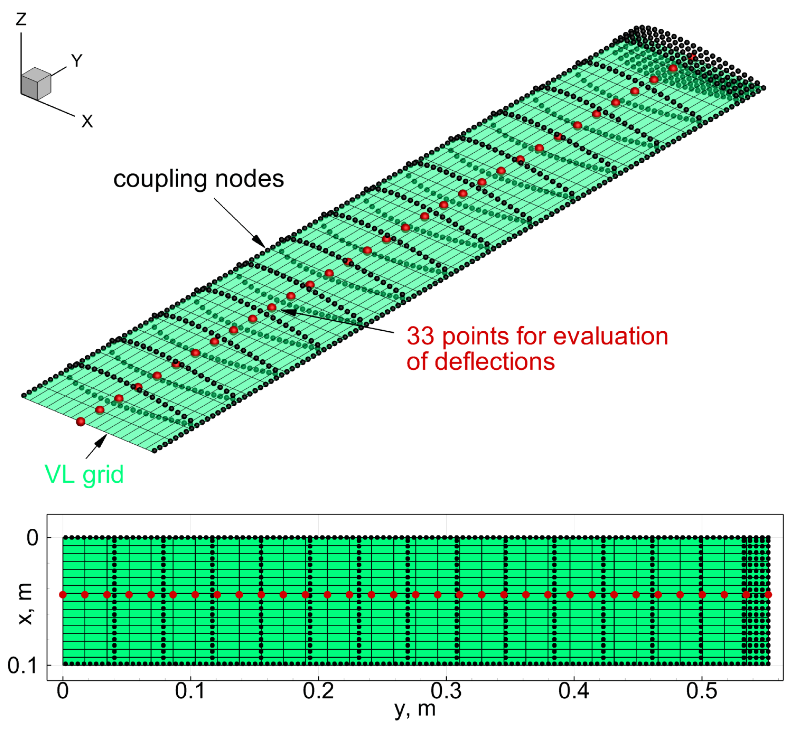
2.1. Implementation of the Steady and Unsteady Vortex Lattice Method

Although a variety of different aerodynamic methods exist, there are several reasons for the usage of a VLM in an aeroelastic toolbox as it is used for the simulations in this paper [21]:
  • It is computationally less expensive and faster than other solutions such as Euler or CFD codes, which typically require high mesh resolutions.
  • The method represents a medium-fidelity tool that incorporates 3D effects and interferences between wakes and lifting surfaces, which are neglected in 2D strip theory.
  • The results are insensitive to large deformations in contrast to the doublet lattice method (DLM), which is a linear method restricted to small out-of-plane displacements.
A detailed description of the underlying principles can be found in the comprehensive work of Katz and Plotkin [22]. The fundamentals, however, are included in the following for the sake of completeness.
Considering the flow conditions of the Pazy wing, low air speeds with Mach numbers below 0.3 and high Reynolds numbers between 105 and 3.5 × 10⁵ are expected. Thus, the flow field can be regarded as incompressible, while viscosity has only a minor influence and can therefore be neglected. Assuming an irrotational and inviscid flow, the velocity at each point of the flow field is obtained by the gradient of the so-called velocity potential ϕ . In combination with the continuity equation, the velocity potential is found by the elliptic differential equation
2 ϕ = 0 ,
which is also known as Laplace’s equation. The solution of this equation leads to a boundary-value problem, whereas for aerodynamic problems, the boundary conditions have to be defined on all solid surfaces and at infinity. For solid walls, the boundary condition is specified so that there is no normal flow through the solid surface on the boundary. The second boundary condition states that the disturbances due to a body moving through a fluid at rest vanish at infinity. By applying one of Green’s identities, a general solution of Laplace’s Equation is possible by using a distribution of elementary solutions, e.g., sources or doublets, on the boundaries of the problem. In the particular implementation used for this work, these so-called singularity elements are vortex rings with constant circulation (VLM of zero order). For the problem solution, it is then only necessary to find a distribution of the singularity elements, which fulfils the (zero) normal flow condition. With the flow field being discretised by singularity elements influencing each other, the problem finally reduces to a set of algebraic equations [9]:
AIC · Γ = RHS .
The normal component of the velocity induced by each element at certain control points, called collocation points, is expressed by the aerodynamic influence coefficients matrix AIC . In general, the calculation of these influence coefficients is based on the Biot-Savart law for the velocity induced at a point P by a straight (uniform strength) vortex segment. On the other hand, the boundary conditions, namely the zero normal flow condition and the Kutta condition, are enforced in the right hand side RHS, which contains all kinematic velocity components of the wing. This includes the rigid body motion of the wing and the velocities induced by the wake vortices, as well as any velocity due to an elastic deformation of the wing or encountered gusts. It is calculated for each panel i as
R H S i = V r b , i + V w a k e , i + V g u s t , i + V e l a s t i c , i · n i ,
with n i being the panel normal vector at the collocation point. Equation (2) is then solved for the unknown circulation Γ i of each panel, which in turn can be used to determine the local pressure distribution and loads.
For the VLM in general, a thin wing planform with infinitesimal thickness and a free wake is assumed. The flow domain is divided into N quadrilateral surface panels and Nw additional wake panels containing rectilinear vortex rings. Each vortex ring consists of a closed vortex line, with the leading segment located on the panel’s quarter chord line and the collocation point at the centre of the three-quarter chord line. The vortex rings are placed on the wing’s camber line of each lifting surface, i.e., no thickness effects are modelled. In case of a steady flow field being examined, the strength of all wake vortex panels is equal to the shedding trailing edge panel. The wake vortices can therefore be seen as horseshoe-like vortices with side vortex lines parallel to the free-stream. In order to describe an unsteady flow field, the solution process presented has to be embedded into a time stepping loop with time step size Δ t . For each time step, a wake panel with a vortex strength equal to its circulation in the previous time step is shed by the trailing edge vortex panel, generating a new row of wake vortex rings. The strength of the wake vortex rings remains unchanged once they have been shed, which inherently fulfils the Kelvin theorem. As the wake shedding procedure becomes computationally demanding with increasing number of time steps and wake length while the influence of the wake rows far behind the wing is negligible, the wake is truncated at a predefined length to save computational costs.
The calculation of the aerodynamic forces F i A in this particular implementation is based on the method by Mauermann [23] and yields [6]
F i A = F S , i A + F U , i A .
The steady forces F S , i A can be calculated by
F S , i A = ρ Γ e f f , i V R B , i + V g u s t , i + V e l a s t i c , i × r i ,
where ρ is the fluid density and r i is a vector of length b equal to the quarter chord line of the corresponding aerodynamic panel i. Furthermore, Γ e f f , i denotes the effective circulation, which is either the difference of the circulation of the corresponding aerodynamic panel and the adjacent panel in chordwise downstream direction, or the circulation of the corresponding panel itself, if the panel is located at the leading edge. The unsteady aerodynamic forces F U , i A are found as
F U , i A = ρ A i Γ i t n i ,
with A i being the area of the i-th panel, Γ i the bound circulation and n i the normal vector. The time derivative of the circulation is discretised by a backward-differential scheme of first order. From Equations (5) and (6), it can be observed that the steady forces act perpendicular to the quarter chord line and the direction of the total velocity vector, while the unsteady forces act along the normal vector of the panel. However, both steady and unsteady forces act at the centre of the panel’s quarter chord line or the centre of each bound vortex ring, respectively.
As the steady aerodynamic forces act perpendicular to the sum of all velocity contributions, no drag components are included in these forces. Instead, the induced drag F D , i A can be calculated separately using the relation [6]
F D , i A = ρ Γ e f f , i V b o d y s t r e a m w i s e , i + V w a k e , i × r i ,
where V b o d y s t r e a m w i s e , i and V w a k e , i denote the velocities induced by the streamwise segments of the bound vortex rings and all segments of the wake vortex rings, respectively. Nevertheless, the VLM does not account for viscous drag forces. This problem can be circumvented, e.g., by approximating the viscous drag forces using the drag polars of the wing’s airfoil [6].
As already mentioned before, the aeroelastic solver used for this work couples the VLM with the commercial FE solver MSC Nastran. Thus, a coupling interface is required to exchange data between both solvers. In addition, the application of two different solvers also leads to the problem of two different and independent models, which means that the aerodynamic forces cannot be applied directly to the structural nodes. This typical problem of fluid–structure interaction (FSI) can be solved using the following relations [6]:
u A = H u S and
F S = H T F A .
The former describes a linear mapping of the displacements of the structural nodes u S to obtain the displacements of the aerodynamic grid points u A using the coupling matrix H . The latter equation is used to transform the aerodynamic forces F A into equivalent forces F S applied to the structural model. For both operations, the same coupling matrix can be used either in normal or in transposed form, taking into account both the global conservation of work as well as the correct description of the structural deformations. Therefore, the coupling matrix of the aeroelastic solver used is based on two- and three-dimensional radial basis functions, which only evaluate the positions of the structural nodes and the aerodynamic grid points. Radial basis functions have become a common tool for multivariate interpolation in fluid–structure interaction, with various functions being available for different applications [24]. In this particular solver, the thin-plate-spline basis function for three-dimensional structural models was implemented [6].

2.2. Linearisation of the Aeroelastic Model

In order to determine the dynamic stability of the Pazy wing, a method for aeroelastic stability analysis of highly flexible wings will be derived in this section. To this end, the whole aeroelastic system is linearised at static equilibrium points with large deformations. At first, the goal is to create a linear state-space model for the aerodynamic model, where equations will be derived from the unsteady VL implementation. Afterwards, the linearisation of the structural response using a modal approach in generalised coordinates is straightforward. Once both aerodynamics and structural dynamics are represented by linear state-space models, these can be combined and integrated into a monolithic linear state-space model to describe the system’s aeroelastic behaviour. However, this paper focuses on the main parts of the linearisation. A detailed description of the derivation can be found in [25].

2.2.1. Derivation of the Linearised Aerodynamic Model

Building a state-space system usually begins with the identification of the state variables of the system. These should allow a complete description of the system’s motion. Considering the aerodynamic model of an aeroelastic system, the relevant variables might be the aerodynamic forces interacting with the structure. In the case of the vortex lattice method, however, it can be seen that the aerodynamic forces are functions of the circulation Γ . The basic formulation of the vortex lattice method in Equation (2) in combination with the RHS vector in Equation (3) yields
AIC · Γ b = RHS = V r b + V w a k e + V g u s t + V e l · n .
Here, Γ b denotes the circulation of bound panels, V r b the rigid body velocity (onflow velocity in a windtunnel test case), while V w a k e and V e l are the velocities induced by the wake and an elastic deformation of the wing. The wake-induced velocities can be calculated as
V w a k e = WIC · Γ w ,
where WIC is called the wake influence coefficients matrix, which is determined in a similar way to the AIC matrix but includes the influence coefficients of the wake vortices with circulation Γ w on the collocation points of the bound vortices. The introduction of Equation (10) into Equation (9) and solving for Γ b leads to
Γ b = AIC 1 · WIC · Γ w + V r b + V e l · n .
Using this equation, the circulation of the bound panels can be expressed by the circulation of the wake panels. Thus, the steady aerodynamic forces A F s , as well as the unsteady aerodynamic forces A F u , can be described as a function of the wake circulation, as will be shown later on. The wake circulations can therefore be regarded as the states that describe the motion of the system. The state vector at the current time step n is accordingly designated Γ w n in the following. At this point, it has to be decided whether the system should be formulated as a discrete-time or continuous-time state-space model. Since the unsteady VLM already uses a time-stepping procedure with discrete time steps, it seems reasonable to use a discrete-time state-space model for the further derivation. In this case, the system is specified to find the solution of the next time step. The evolution of the wake circulation is defined by the wake-shedding process that is described in Section 2.1 and consists of two different operations. In the first step, the wake vortex rings are shifted by one panel in the downstream direction and a new row of wake vortex rings is created at the trailing edge of the wing. Afterwards, the circulation from the wing trailing edge row is transferred to this new wake row. This routine can be written as
Γ w n + 1 = M b · Γ b n + M w · Γ w n ,
where M b is the matrix for transferring the bound circulation from the trailing edge row and M w is the matrix for shifting the wake rows. The result of this equation is the wake circulation at the next time step Γ w n + 1 . Substitution of Γ b using Equation (11) results in
Γ w n + 1 = M b · AIC 1 · WIC · Γ w n + V r b + V e l · n + M w · Γ w n ,
with M b , M w , AIC 1 and WIC being constant matrices. Hence, the wake circulation Γ w n + 1 during the next time step is only a function of the current wake circulation Γ w n , the velocities V r b and V e l , as well as the panel normal vectors n . Referring to the basic formulation of discrete-time state-space models, which is
x n + 1 = Ax n + Bu n ,
only the variables of the input vector u n have to be defined, since the state vector x n has already been designated as Γ w n . Accordingly, only the velocities V r b , V e l and the panel normal vectors n are available as input variables. As the model will be used to describe the dynamic behaviour at a static aeroelastic equilibrium, the rigid body velocity V r b can be assumed constant. For this reason, the velocity V e l and the panel normal vectors n are chosen to be part of the input vector due to the elastic motion of the wing, while V r b will be included in the control matrix B . Equation (13) can then be rewritten in matrix notation:
Γ w n + 1 = M w M b · AIC 1 · WIC · n A A · Γ w n A x + M b · AIC 1 · c V r b M b · AIC 1 · n A B · n c V e l n A u .
This equation describes a state-space system in discrete-time formulation, as shown in Equation (14). The index c indicates that the velocities are related to the collocation points of the aerodynamic panels. It can be seen that n appears both in the A A and in the A B matrix, although it is defined as an input of the system. Due to the linear character of the system, the amplitudes of the described motion and thus the changes in the normal vectors are assumed to be small. In this case, the assumption of constant normal vectors in matrices A A and A B seems appropriate. Furthermore, the effect of a change in the normal vectors is also taken into account, since n is a part of the input vector. The behaviour of the system’s states over time can now be determined completely using the equation
Γ w n + 1 = A A · Γ w n + A B 1 A , c B 2 · n c V e l n ,
where A A R n w × n w and A B R n w × 6 n b are referred to as aerodynamic dynamics and input matrix, while A x R n w and A u R 6 n b are the aerodynamic state and input vector, respectively. Furthermore, n b denotes the number of bound panels and n w the number of wake panels.
It is now possible to describe the resulting aerodynamic forces as outputs of the state-space system, according to the relation
y n = Cx n + Du n .
In the unsteady vortex lattice solver that was used, the total forces are the sum of the steady and unsteady aerodynamic forces. The steady aerodynamic forces A F s are given by
A F s , i = ρ · Γ e f f , i · V r b , i + V e l , i + V g u s t , i × r i .
The index i, representing the number of the (bound) aerodynamic panel considered, is disregarded in the following for the sake of simplification. The effective circulation Γ e f f is defined as the difference of the circulation of the corresponding aerodynamic panel and the adjacent panel in chordwise downstream direction, except for the panels at the leading edge. It is calculated from the bound circulation using
Γ e f f = M e f f · Γ b ,
where M e f f R n b × n b . Introducing Equation (19) together with Equation (11) into Equation (18) and rearranging the equations results in
A F s n = A C s · Γ w n + A D s , 1 A , q D s , 2 + A , c D s , 2 A D s , 3 · n q | c V e l r n .
As can be seen, the steady forces depend on the state variables Γ w and the input variables V e l and n . In addition, the vector r , pointing in the direction of the quarter chord line of the aerodynamic panels, is now also part of the input vector. The index q is introduced as the velocities for calculating the aerodynamic forces are evaluated at the quarter points of the panels. The steady aerodynamic sensor matrix A C s and the sub-matrices of the steady aerodynamic direct term A D s are defined by
A C s = ρ · r ˜ s k e w · q V ˜ r b · M e f f · AIC 1 · WIC * R 3 n b × n w ,
A D s , 1 = ρ · r ˜ s k e w · q V ˜ r b · M e f f · AIC 1 · c V ˜ r b T R 3 n b × 3 n b ,
A , q D s , 2 = ρ · M e f f · AIC 1 · c V ˜ r b T · n ˜ · r ˜ s k e w R 3 n b × 3 n b ,
A , c D s , 2 = ρ · r ˜ s k e w · q V ˜ r b · M e f f · AIC 1 · n ˜ T R 3 n b × 3 n b ,
A D s , 3 = [ ρ · M e f f · AIC 1 · ( WIC * · Γ ˜ w 0 · V ˜ r b , s k e w + V ˜ r b T · n ˜ · V ˜ r b , s k e w ) ] R 3 n b × 3 n b ,
with WIC * = WIC · n .
Here, the vectors q | c V r b , n and r are transformed into the equivalent matrices q | c V ˜ r b , n ˜ and r ˜ containing the entries for each panel blockwise in diagonal form. In order to evaluate the cross-product between the velocities and the vector r (cf. Equation (18)), these appear as skew-symmetric matrices in some places. At this point, it has to be mentioned that the steady wake circulation Γ ˜ w 0 obtained from the steady-state solution at static aeroelastic equilibrium is included in the direct term A D s , 3 . This is the case since aerodynamic forces are always follower forces, and thus, any deformation of the wing will generate additional loads as the direction of forces changes with the lifting surface (in this case expressed by the vector r ). The impact of steady aerodynamic loads on the aeroelastic stability is particularly important in the context of T-tail flutter [26] but can also influence the stability of flexible wings with large deformations, as will be shown later.
While the steady forces depend on the bound circulation in the original vortex lattice implementation, the unsteady aerodynamic forces A F u depend on the time derivative of the bound circulation rather than on the bound circulation itself. These can be determined using the relation
A F u = ρ · A p · Γ b t · n ,
where A p denotes the panel areas of the corresponding bound panels. Again, Equation (11) can be introduced into this equation, resulting in the unsteady forces being described as a function of the state and input vectors as well as their first time derivatives. While the latter are regarded as additional inputs to the system, the time derivative of the wake circulation is calculated using the first-order forward scheme
Γ w t Γ w n + 1 Γ w n Δ t ,
with Δ t being the time step size. In order to use this scheme in a discrete-time state-space formulation, the time derivative is now calculated by the difference between the next time step n + 1 and the current time step n. By substituting Γ w n + 1 using Equation (16) and further arrangements, the unsteady forces can be expressed as
A F u n = A C u · Γ w n + A D u , 1 A , c D u , 2 0 A D u , 4 A , c D u , 5 · n c V e l r n ˙ c V ˙ e l n .
Five instead of three different input variables are included in this equation. However, the state vector only contains the wake circulation Γ w , and the corresponding unsteady aerodynamic sensor matrix A C u is
A C u = ρ · 1 Δ t · n ˜ · A ˜ p · AIC 1 · WIC * · A A I R 3 n b × n w ,
where I denotes an identity matrix. The sub-matrices of the unsteady aerodynamic direct term A D u can be determined by
A D u , 1 a = ρ · 1 Δ t · n ˜ · A ˜ p · AIC 1 · WIC * · A B 1 R 3 n b × 3 n b ,
A D u , 1 b = ρ · 1 Δ t · A ˜ p · AIC 1 · WIC * · A B 1 · n ˜ R 3 n b × 3 n b ,
A D u , 1 c = ρ · 1 Δ t · A ˜ p · AIC 1 · WIC * · A A I · Γ w 0 R 3 n b × 3 n b ,
A , c D u , 2 = ρ · 1 Δ t · n ˜ · A ˜ p · AIC 1 · WIC * · A B 2 R 3 n b × 3 n b ,
A D u , 4 a = ρ · n ˜ · A ˜ p · AIC 1 · c V ˜ r b T R 3 n b × 3 n b ,
A D u , 4 b = ρ · n ˜ · A ˜ p · AIC 1 · WIC · Γ w 0 R 3 n b × 3 n b ,
A , c D u , 5 = ρ · n ˜ · A ˜ p · AIC 1 · n ˜ T R 3 n b × 3 n b .
Again, the effect of the steady loads is taken into account by including the steady wake circulation in matrices A D u , 1 c and A D u , 4 b . Finally, the total aerodynamic force vector A F is obtained from the sum of steady and unsteady forces:
A F n = A C s + A C u · Γ w n + A D s , 1 + A D u , 1 A , q | c D s , 2 + A , c D u , 2 A D s , 3 A D u , 4 A , c D u , 5 · n q | c V e l r n ˙ c V ˙ e l n .
As can be seen, the calculation of drag forces has not yet been considered in the linearisation of the aerodynamic forces. The reason for this is that the induced drag—according to its definition in Equation (7) and with the current formulation of the state-space model—would depend quadratically on the state and input variables. A similar problem was encountered for several higher-order terms in the steady and unsteady forces, which could not be modelled by a linear system and therefore had to be neglected in the linearisation. The steady-state induced drag included in the steady loads at static aeroelastic equilibrium, however, will be integrated into the monolithic aeroelastic state-space model presented in the following section.

2.2.2. Derivation of the Linearised Aeroelastic Model

In contrast to the derivation of the aerodynamic model, the derivation of the linear structural model is straightforward and is widely presented in the literature. A detailed description of the linearisation process is therefore omitted at this point but can be found, e.g., in [27]. Considering the second-order structural equation of motion in generalised coordinates with inertia, stiffness and (rayleigh) damping terms, this equation can be expressed by
q ˙ 1 , i q ˙ 2 , i = 0 1 Ω i D i S A · q 1 , i q 2 , i S x + 0 Φ i T S B · S F S u ,
i = 1 , 2 , , n m ,
which is a linear continuous-time state-space system of the form x ˙ = A x + B u . Here, Ω i are the squares of the natural frequencies ω i and Φ i are the mass-normalised eigenvectors of each mode i. In order to account for the effect of geometric nonlinearities, the eigenfrequencies and eigenvectors are obtained from an eigenvalue analysis of the preloaded structure. The number of modes considered is designated n m , S A R 2 n m × 2 n m denotes the structural dynamics matrix and S B R 2 n m × 3 n f e the structural control matrix, where n f e is the number of FE nodes. The state vector S x R 2 n m contains the generalised coordinates q 1 for the considered modes and the first time derivatives of the generalised coordinates q 2 which can be seen as the generalised velocities. The structural input vector S F R 3 n f e includes the structural force components acting on all nodes of the finite element model.
In order to merge both linearised models, the structural model needs to be transformed from continuous into discrete-time formulation. The conversion is done by means of the so-called matrix exponential, and the equivalent discrete-time system of the structural model yields
q 1 q 2 n + 1 = e Δ t · S A S A ¯ · q 1 q 2 n + S A 1 · e Δ t · S A I · S B S B ¯ · S F n ,
with Δ t representing the desired time step size. The integration of both the structural and the aerodynamic model into a monolithic aeroelastic state-space system is performed by expressing the inputs of one system with the states of the other system. Recalling Equations (16) and (37) of the aerodynamic model, the inputs are the quarter-chord line vectors r , the panel normal vectors n , the elastic velocity V e l and their time derivatives n ˙ and V ˙ e l , respectively. It is obvious that the normal vectors change depending on the deformation of the wing, where the deformation can be directly expressed using the modal approach. The normal vectors, however, are determined using the relation
n = i = 1 n m n Φ i · q 1 , i ,
where n Φ i is the partial derivative of the panel normal vectors with respect to the eigenvectors of the i-th mode. This expression describes the change in n due to a small excitation of each mode around the static aeroelastic equilibrium. Since no analytical approach for the calculation of the partial derivative was found, the derivative is determined by a finite-difference approach during preprocessing. The quarter-chord line vectors r are also only dependent on the grid deformation and are thus defined in a similar manner as the normal vectors in Equation (40).
The elastic velocity V e l is obtained using the modal approach, but with the generalised velocity q 2 instead of the generalised deflection q 1 . In this context, two problems are encountered due to the different models of the solution methods. The resulting physical coordinates are still related to the structural grid describing the motion of the FE nodes, while the inputs V e l need to be defined at the collocation points of the aerodynamic grid. Therefore, the velocities have to be interpolated onto the aerodynamic grid points using the coupling interface introduced in Section 2.1. Afterwards, the elastic velocities must be interpolated from the aerodynamic grid points to the collocation points. Thus, the velocities due to the elastic deformation of the wing can be expressed by
c V e l = M c p · H d · Φ · q 2 ,
where H d denotes the coupling matrix for mapping displacements between structural and aerodynamic grid, and M c p is a matrix for interpolation from the aerodynamic grid points to the collocation points. Using these new relations for n and V e l , the evolution of the aerodynamic state vector can finally be written as
Γ w n + 1 = A A A 11 A B 1 · n Φ A 12 A , c B 2 · M c p · H d · Φ A 13 · Γ w q 1 q 2 n .
Thus, the aerodynamic states at the next time step now only depend on the extended dynamics matrix, including the additional sub-matrices A 12 and A 13 of dimension n w × n m . Furthermore, the state vector has been expanded by the two generalised coordinates of the structural state vector.
The integration of the structural model is performed similarly to the aerodynamic model. In this case, the structural forces S F are derived from the resulting total aerodynamic forces A F by
S F = H f T · A F ,
where H f is the coupling matrix for transferring the forces from the aerodynamic grid to the structural grid. In contrast to the integration of the aerodynamic model, two additional input variables must be handled for the integration of the total aerodynamic forces into the structural model. The time derivative n ˙ of the panel normal vectors is obtained similar to Equation (40) using the modal approach with the generalised velocity q 2 . Accordingly, the elastic acceleration V ˙ e l can be expressed in a similar way as the elastic velocity V e l by the generalised acceleration q 3 . By means of these relations, the aerodynamic forces are defined as functions of the aerodynamic and structural states and are introduced into the structural state-space system. As both aerodynamic and structural model are now related to the same state vector, they can be finally merged to build a linear, discrete-time state-space model for the entire aeroelastic system:
Γ w q 1 q 2 q 3 f d n + 1 = A 11 A 12 A 13 0 0 A 21 A 22 A 23 A 24 A 25 A 31 A 32 A 33 A 34 A 35 A 41 A 42 A 43 0 0 0 0 0 0 I · Γ w q 1 q 2 q 3 f d n .
Using this equation, it is possible to describe the aeroelastic behaviour of a highly flexible wing at any deformed state of steady aeroelastic equilibrium. In general, the state vector of this system is of dimension R n w + 4 n m , i.e., the number of wake panels plus four times the number of modes considered in the modal approach. Here, the discrete-time formulation is favourable in terms of verification as it allows for time-marching and straightforward comparison with reference results from solvers in the time domain. Besides these advantages, the unsteady VLM used for the derivation of the linear aerodynamic model is already formulated in discrete time. As the linear structural model is originally formulated in continuous time, one of both models has to be converted for the integration of both models into a monolithic state-space model. The transformation of a continuous into a discrete time model using the matrix exponential, however, is much easier than vice versa. Since the generalised acceleration q 3 is not provided by the linearised structural model in discrete-time formulation (cf. Equation (39)), it is approximated from the generalised velocity q 2 by
q 3 n + 1 q 2 n + 1 q 2 n Δ t ,
which represents a first-order backward scheme to account for the state-space formulation of q 3 at the next time step. Both components of this equation are included in the aeroelastic state-space model and can be easily expressed by the third line of Equation (44). The integration of this additional state is important for modelling the elastic acceleration V ˙ e l , which is mandatory since it accounts for almost half of the unsteady forces (depending on the reduced frequency) [25]. Besides, the steady induced drag is also taken into account by means of the generalised (structural) drag forces f d , which are obtained from the induced (aerodynamic) drag forces A F d at static aeroelastic equilibrium using
f d = Φ T · H f · A F d .
However, as can be seen from Equation (44), these forces do not change dynamically but are added as a static component to the system to prevent possible instabilities of modes involving in-plane motions. The consideration of viscous forces has not yet been integrated, but could be realised in a similar way as the induced drag, i.e., using a static state that only accounts for the viscous drag at steady aeroelastic equilibrium. In the existing VL implementation, the viscous forces can be approximated using drag polars of the wing’s airfoil, where the results showed good agreement with CFD results for steady simulations [1].
For the verification of both the aerodynamic and the aeroelastic state-space model, the results of time-domain simulations for generic test cases are compared to results from an existing unsteady VL solver and a nonlinear aeroelastic modal solver. A detailed description of the verification process can be found in [25]. The results of the verification test case for the undeformed (0° AoA) Pazy wing structural model are presented in Figure 1, which depicts the evolution of the unsteady forces and the generalised coordinates over time for a free vibration of the wing due to small disturbances. These disturbances are realised by a small deformation of the wing, which can be achieved by setting an initial value for the generalised coordinate q 1 . For simplification, only the lowest four natural modes are taken into account, which are the first ( q 1 , 1 ), second ( q 1 , 2 ) and third ( q 1 , 4 ) out-of-plane bending modes as well as the first torsion mode ( q 1 , 3 ). For this case, the results agree very well for the three bending modes. Considerable differences appear in the evolution of the first out-of-plane bending DOF ( q 1 , 1 ). However, since these differences occur mainly at the beginning of the simulation, they may be caused by an issue regarding the unsteady forces in the modal solver. These are determined using a first order backward scheme, which results in significantly larger forces for the first time step. Other reasons might be the force terms neglected during the linearisation and, of course, the fact of comparing the solution of a linear state-space model to a fully nonlinear modal solver also accounting for geometric nonlinearities.

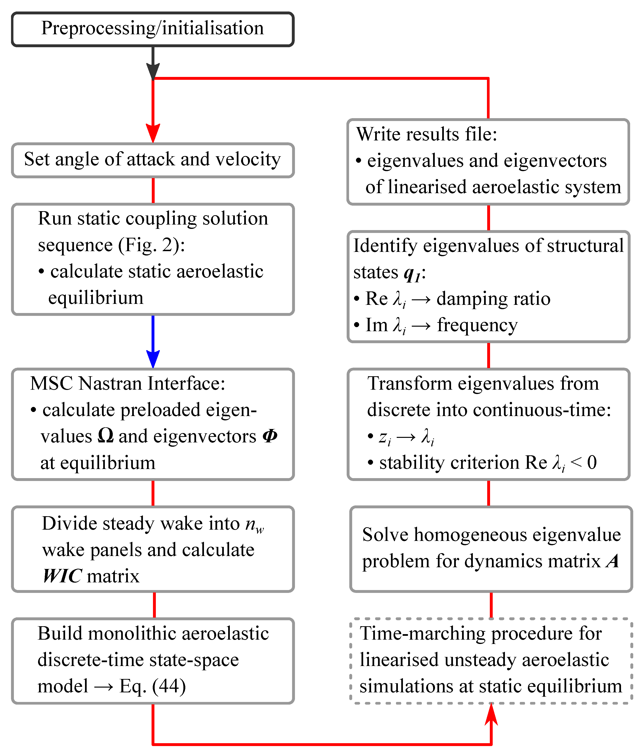
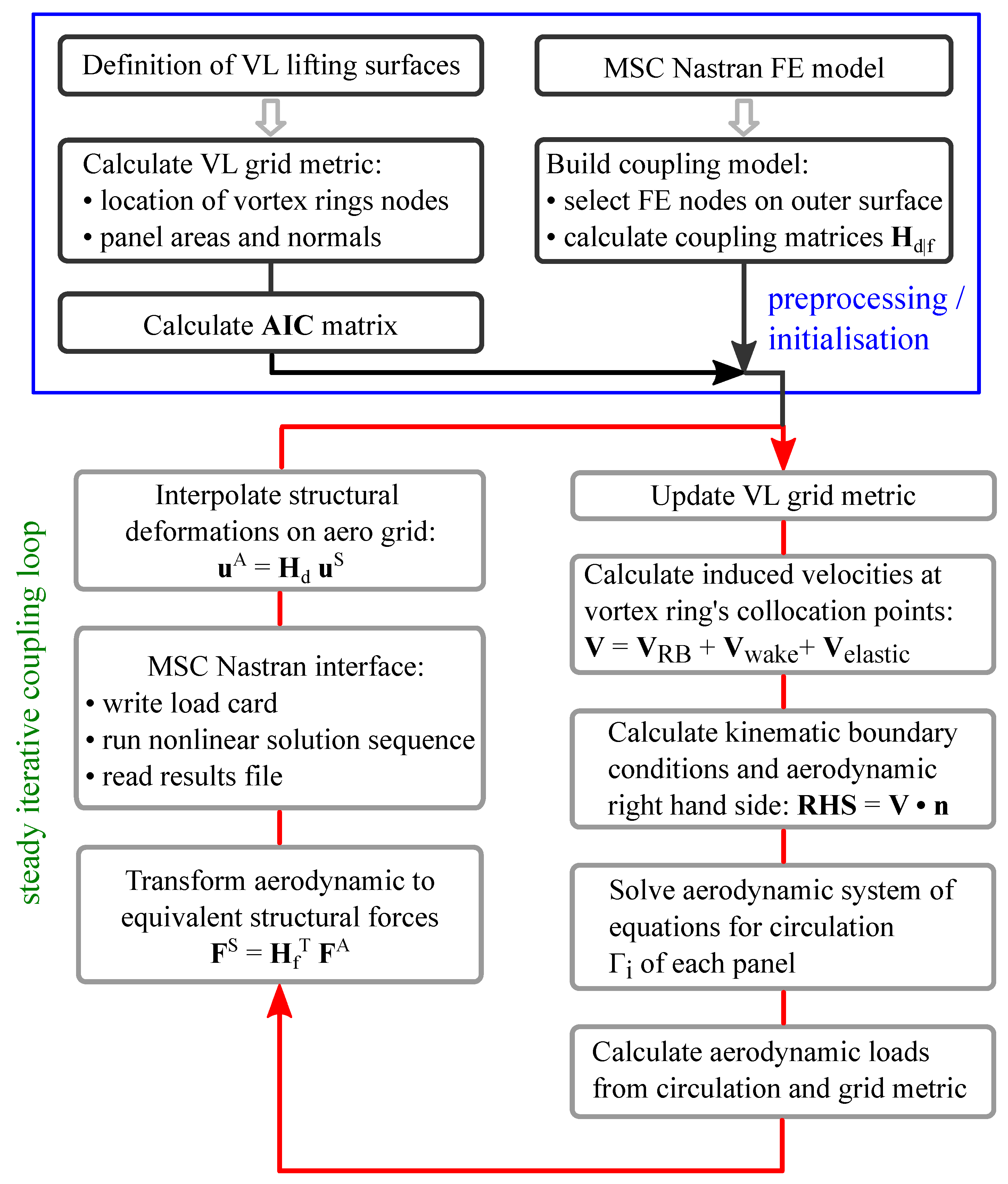
2.3. Aeroelastic Framework and Solution Sequence

The aeroelastic simulations used to determine the steady static equilibrium points are performed by applying a steady iterative coupling loop. Here, the aerodynamic solution is obtained by the steady vortex lattice implementation, whereas the structural solution is computed separately using the MSC Nastran FE solver. The general workflow of the static coupling solution sequence is illustrated in Figure 2. In addition to the setup of the aerodynamic model, the initialisation process also includes the setup of the FE model and the coupling model as a preprocessing step. The aerodynamic forces are calculated as a function of the circulation and transformed into equivalent structural forces. Since a partitioned approach is used for solving the FSI problem in this aeroelastic framework, interface functions are available to provide the Nastran loadcard and read the results file of the nonlinear SOL400 sequence. Convergence is checked in terms of structural displacements, and the iterative loop is stopped once a specified residuum is reached. Before each new iteration loop, the VL grid as well as the coupling matrix and the AIC matrix are updated with respect to the structural deformations.
The stability analysis of the aeroelastic system is preferably described using the flowchart of the linearised static coupling solution sequence in Figure 3. When convergence of the static coupling loop is reached, the structural solution using Nastran SOL400 is extended by a modal analysis on the preloaded structure following the nonlinear static analysis. Subsequently, the wake of the steady solution, which consists only of one row of long wake vortex rings, is divided into a number of equal-length wake rows to obtain a wake similar to that of an unsteady solution. The stability of the aeroelastic system is evaluated by solving the homogeneous eigenvalue problem for the dynamics matrix of the monolithic state-space model. In this particular case, the complex eigenvalues obtained appear in the discrete-time form z, and the system is only stable if the magnitudes of all eigenvalues are smaller than one (eigenvalues located inside the unit circle in the complex z-plane). As this representation is not suitable for common illustration methods, such as root-locus or V-g and V- ω plots, the eigenvalues are converted into continuous-time form by [21]
λ i = log z i Δ t .
Afterwards, the real parts of the eigenvalues represent the decay ratios and the imaginary parts represent the frequencies of the system’s modes. The system is then regarded as internally stable, if all eigenvalues λ i have a strictly negative real part [27]. In summary, the presented method for stability analysis accounts for all three nonlinear effects involved in highly flexible wings undergoing large deformations. This includes the change in structural eigenvalues and eigenvectors due to the deformation, the change in the AIC matrix due to varying wing geometry, as well as the effect of steady aerodynamic loads at aeroelastic equilibrium.

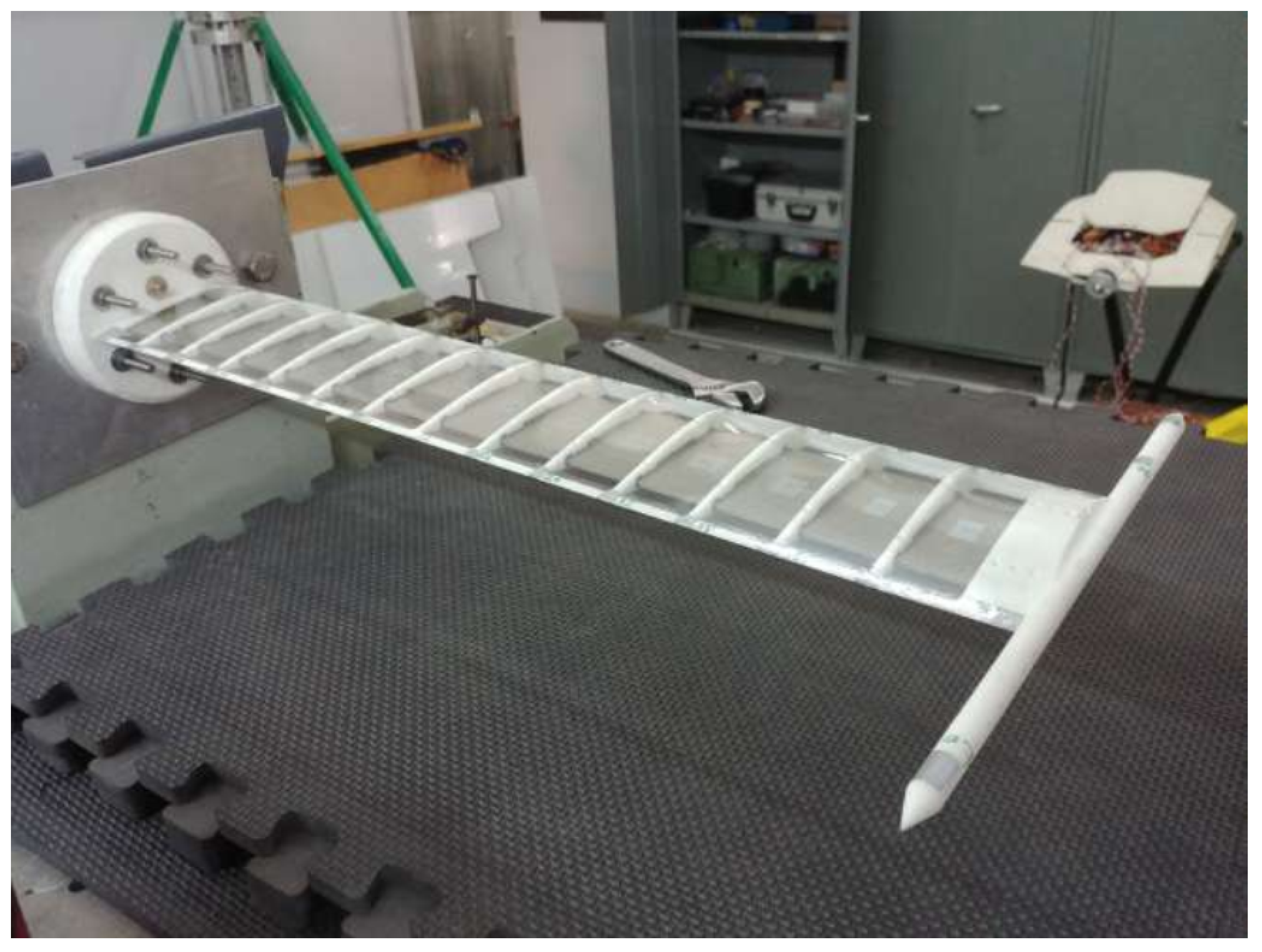
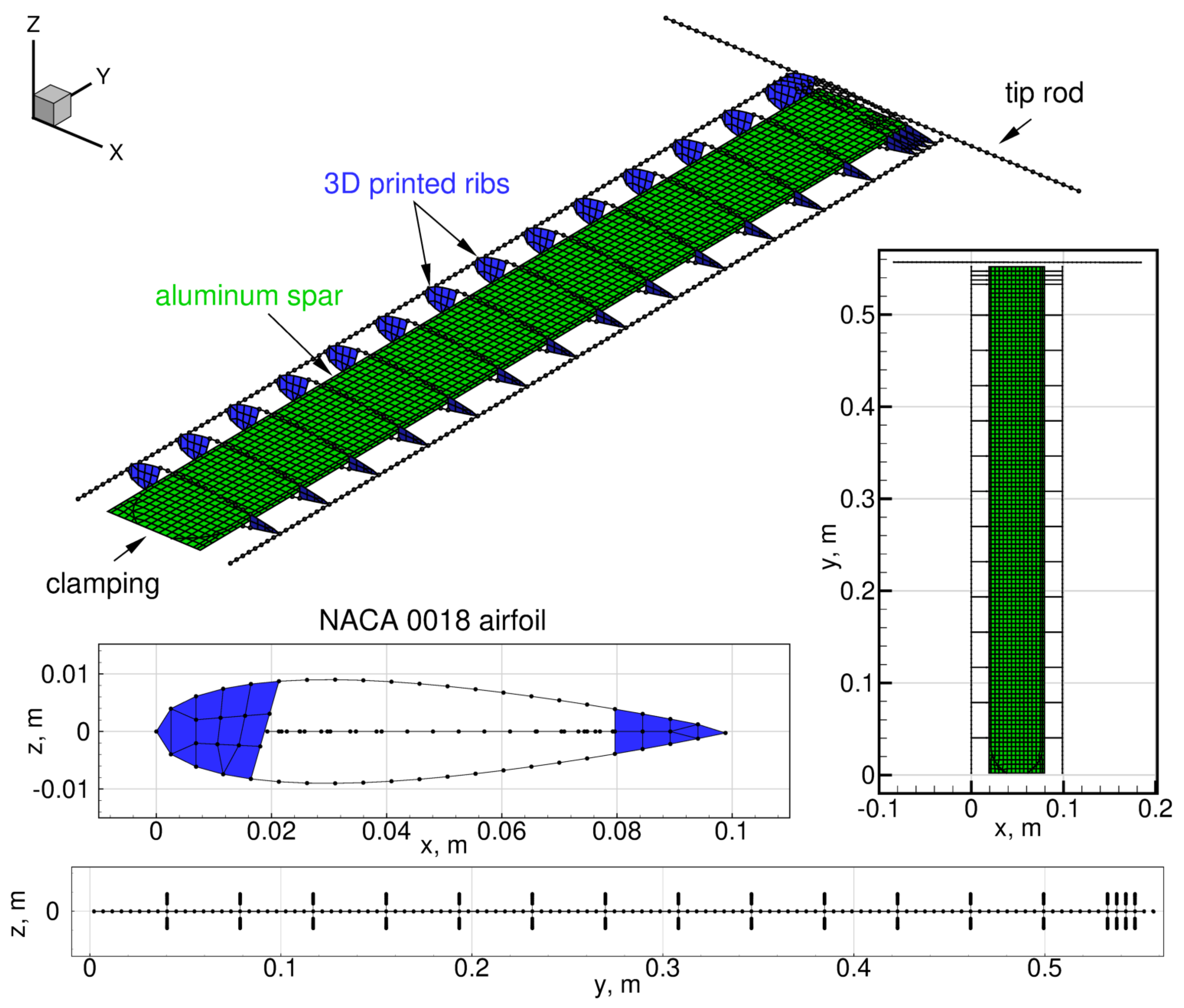
2.4. Structural and Aerodynamic Simulation Models

The Pazy wing aeroelastic benchmark was primarily designed to undergo very large deformations of up to 50% in wind-tunnel tests. Two different models were built, whereas two ribs were added at the wing root of the second model. While the design has not been changed for the most part, both models slightly differ in terms of their natural frequencies. Unfortunately, the first model, called Pre-Pazy wing, was destroyed early during a wind-tunnel test campaign, so experimental data are only available for the second model. The simulations in this work, however, are performed exclusively for the Pre-Pazy wing, as the FE model for the second wing was not yet available at the beginning of these studies.
The wing, shown in Figure 4, has a span of 550 mm and a chord length of 100 mm with a symmetric NACA 0018 airfoil. It is assembled from an Aluminum 7075 spar and a PA2200, 3D printed rib structure. This is covered by an Oralight polyester film, which is applied by ironing and shrinks once the heat source is removed, resulting in a prestressing of the foil. This approach is chosen to ensure a smooth surface of the closed profile around the wing and to prevent buckling even at states of large deformations. As can be seen, a wing-tip rod is part of the 3D printed chassis, which can be used for attaching weights to modify the structural characteristics and thus the dynamic behaviour and the flutter speed. Important aerodynamic and geometrical properties of the Pazy wing are listed in Table 1, while a detailed description of the wing can be found in references [2,28].
The Nastran FE model, as illustrated in Figure 5, is provided by Technion and is publicly available for participants of the AePW3. It is composed of beam elements (CBEAM) modelling the leading edge, trailing edge and the tip rod, as well as shell elements (CTRIA3, CQUAD4) used to model the main spar and the Oralight skin. The ribs consist of a combination of beam and shell elements. Unfortunately, the shell elements do not account for the prestressing of the skin, which causes buckling and convergence issues in nonlinear structural analyses even at very low loadings. Therefore, the simulations in this work are performed for a modified model, where the shell elements representing the skin have been removed. Regarding the coupling interface between the FE and the VL grid described in Section 2.1, a set of structural nodes must be defined for the transfer of forces and the interpolation of deformations. In this particular case, the 952 nodes selected include the nodes of the outer ribs, the leading and the trailing edge. These coupling nodes and the VL grid are depicted in Figure 6 and show a good match, which is important for a correct data exchange between both models.

3. Numerical Simulations and Results

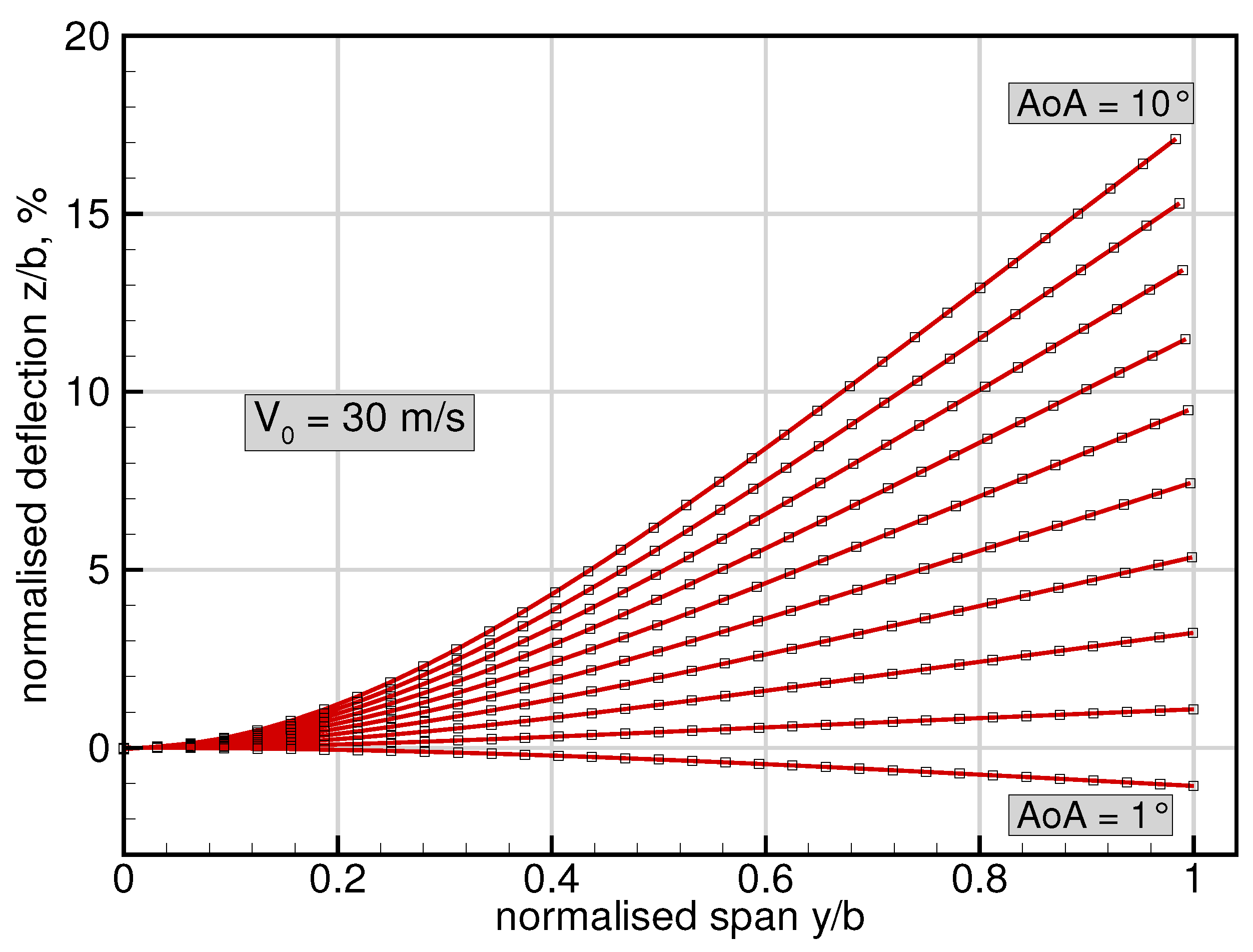
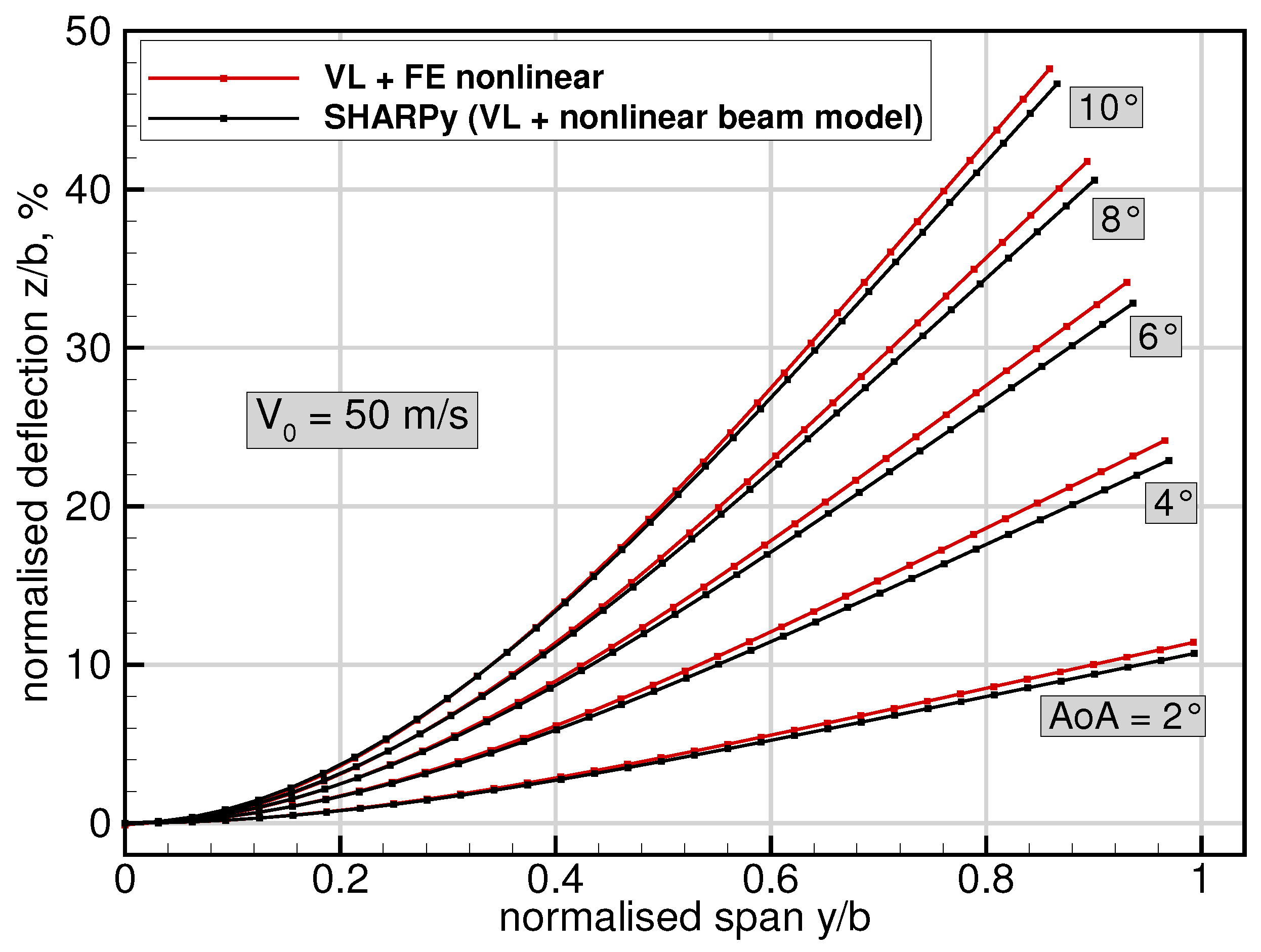
3.1. Static Coupling Simulations

Static coupling simulations are performed for velocities of 30, 40 and 50 m/s and angles of attack ranging from 1 to 10 degrees. Although the wind tunnel tests are also performed with lower flow velocities, these conditions have been chosen to consider the effects of geometric nonlinearities. The density is set to 1.225 kg/m3 at mean sea level. For the steady VL solution, the wing is discretised with 16 chordwise and 32 spanwise equidistant panels. Although the wing is fixed vertically in the wind tunnel test, the direction of gravity is assumed along the negative z direction. This is the case since the simulation setup is mainly based on the setup of the Imperial College group [29], another member of the LDWG, in order to achieve the best possible comparability. The most important parameters are shown in Table 2.
The results of the structural deformations at 30 m/s onflow velocity are shown in Figure 7, where the normalised out-of-plane deflection Δ z with respect to the wing span is plotted over the normalised spanwise coordinate y / b . For simplification of further comparisons, the deformations are evaluated at 33 equidistant points in the spanwise direction, which are located at 44.75% chord (see Figure 6). This location was chosen as the results from Imperial College were obtained from SHARPy (Simulation of High-Aspect Ratio aeroplanes in Python [30]), which uses a nonlinear, geometrically exact beam formulation, where the beams’ elastic axis in the Pazy wing structural model is placed at this exact position. For an angle of attack of 1 degree, the wing exhibits negative deformation due to the gravity forces outweighing the aerodynamic lifting loads. From 2 degrees of angle of attack on, the deformations become positive and—as expected—increase with each increment in angle of attack. The maximum wing tip displacement in the z direction of approximately 17% is obviously achieved at 10 degrees angle of attack. The influence of geometric nonlinearities can be roughly estimated from the tip displacement in the spanwise (y) direction. In this case, the influences seem to be rather small, as the maximum spanwise displacement is approximately 2% with respect to the span of the wing. It can also be seen that the curvature due to bending mainly occurs between the clamping and about 40% span, while the remaining part of the outer wing shows only minor local out-of-plane bending deformations.
The results for five angles of attack at the highest onflow velocity of 50 m/s are depicted in Figure 8. With a maximum tip displacement of approximately 47% in the z direction and 14% in the y direction, the deformations obviously are in a nonlinear regime, and it becomes apparent that the application of a geometrically nonlinear solution method is indispensable here. While a geometrically linear solution at velocities below 30 m/s might only lead to small deviations, in this case it would clearly lead to an arbitrary extension of the wing’s span and in turn to an increase of the wing area by more than 14%. This would finally result in a significantly different lift distribution and deformation of the wing. Furthermore, it can be seen that the deflections obtained from SHARPy provided by Imperial College appear to be smaller with an almost constant deviation of 1.2% normalised deflection in the z direction between 4 and 8 degrees angle of attack. One reason for these differences can be the different positions of the elastic axis in both models. While the axis of the beam model remains constant at 44.75% chord, the axis of the full 3D FE model changes slightly with respect to the spanwise coordinate, thus leading to a different distribution in the torsional moment. However, the main reason for the deviations is still found in the different structural solution methods, where, for example, a change of camber of the wing due to the natural coupling of out-of-plane and in-plane bending deformations is not accounted for in a beam model. Previous validations of the static coupling solver with results from a nonlinear, strain-based beam solver for a similar test case (up to 35% displacement with respect to semi-span) have shown comparable deviations in terms of out-of-plane displacements (see [6]).
In addition to the results from Imperial College, the static coupling simulation results are also compared to the few experimental data available from Technion for the Pre-Pazy wing, as shown in Table 3. In this case, the simulation setup (cf. Table 2) is modified in terms of the direction of gravity, since the wing is fixed vertically in the windtunnel (i.e., gravity in neg. y direction). It should also be noted that the simulations are carried out using the FE model without skin due to the convergence issues mentioned in Section 2.4. As can be seen, this circumstance leads to an overestimation of the tip displacement obtained from the simulation with deviations of approximately 15% between simulation and experiment for the 5 degree AoA cases. This can clearly be related to the stiffness of the skin, which is not accounted for in the FE model, resulting in a less rigid wing. Interestingly, the differences are reduced to 5% for the test case with large deformations.

3.2. Influence of Geometric Nonlinearities on Modal Properties

In the previous section, it has been shown that structural deformation is a key parameter for the Pazy wing test case. The consideration of large structural deformations also leads to a change in structural properties, i.e., the stiffness expressed by the updated (tangent) stiffness matrix. With regard to the large static deflections at high angles of attack and high onflow velocities, it can be expected that the modal properties (eigenvalues, eigenvectors) will change significantly. In order to evaluate these changes, the eigenvalues or eigenfrequencies, respectively, are analysed as a function of the deformation. For this purpose, the extended static coupling solver as implemented for the stability analysis is used, with data being obtained from a Nastran SOL400 modal analysis performed after convergence of the static coupling solution. Here and in the following, only modes in a meaningful frequency range of up to 150 Hz are taken into account. Thus, the first out-of-plane bending (1st OOP), the second out-of-plane bending (2nd OOP), the first torsion (1st Torsion), the third out-of-plane bending (3rd OOP), the first in-plane bending mode (1st IP) and two other modes are considered. The latter are the second torsion (2nd Torsion) with contributions from the 3rd OOP bending mode and vice versa.
The development of the eigenfrequencies as a function of the normalised tip displacement is plotted in Figure 9 for two different angles of attack and velocities ranging from 10 to 90 m/s. Here, the frequencies of the 1st OOP and the 2nd OOP bending mode remain almost constant, indicating that these modes are comparatively insensitive to the elastic structural deflection. On the other hand, significant changes are observed in the frequency of the 1st Torsion, which begins to decrease considerably at 10% tip displacement and reaches the same value as the 2nd OOP bending mode at approximately 31% tip displacement and 50 m/s onflow velocity. At higher velocities, the frequency keeps decreasing and approaches the frequency of the 1st OOP bending mode. A similar behaviour is shown for the 1st IP bending mode, where a major frequency drop is already observed at small tip displacements but stabilises above 30% deformation. The frequencies of the two highest modes are increasing at small deformations, while they seem to be minorly affected at larger displacements. Concerning the mode shapes, it has to be noted that the 1st IP bending mode shows contributions of the 1st Torsion and vice versa as soon as small elastic deformations occur. This might be a reason for the frequency drop of the 1st IP mode even at small displacements. However, the behaviour of the 1st Torsion frequency seems to be primarily affected by geometric nonlinearities, since changes occur mainly in a nonlinear regime above 10% tip displacement. Although no unsteady aerodynamic forces have been considered yet, it can be assumed that coupling of the 1st Torsion and the 2nd OOP bending mode will lead to aeroelastic instabilities. As no differences are observed between 3- and 5-degree angle of attack, it can be concluded that the eigenvalues are not affected by different lift distributions (for same total lift), but only depend on the tip displacement.

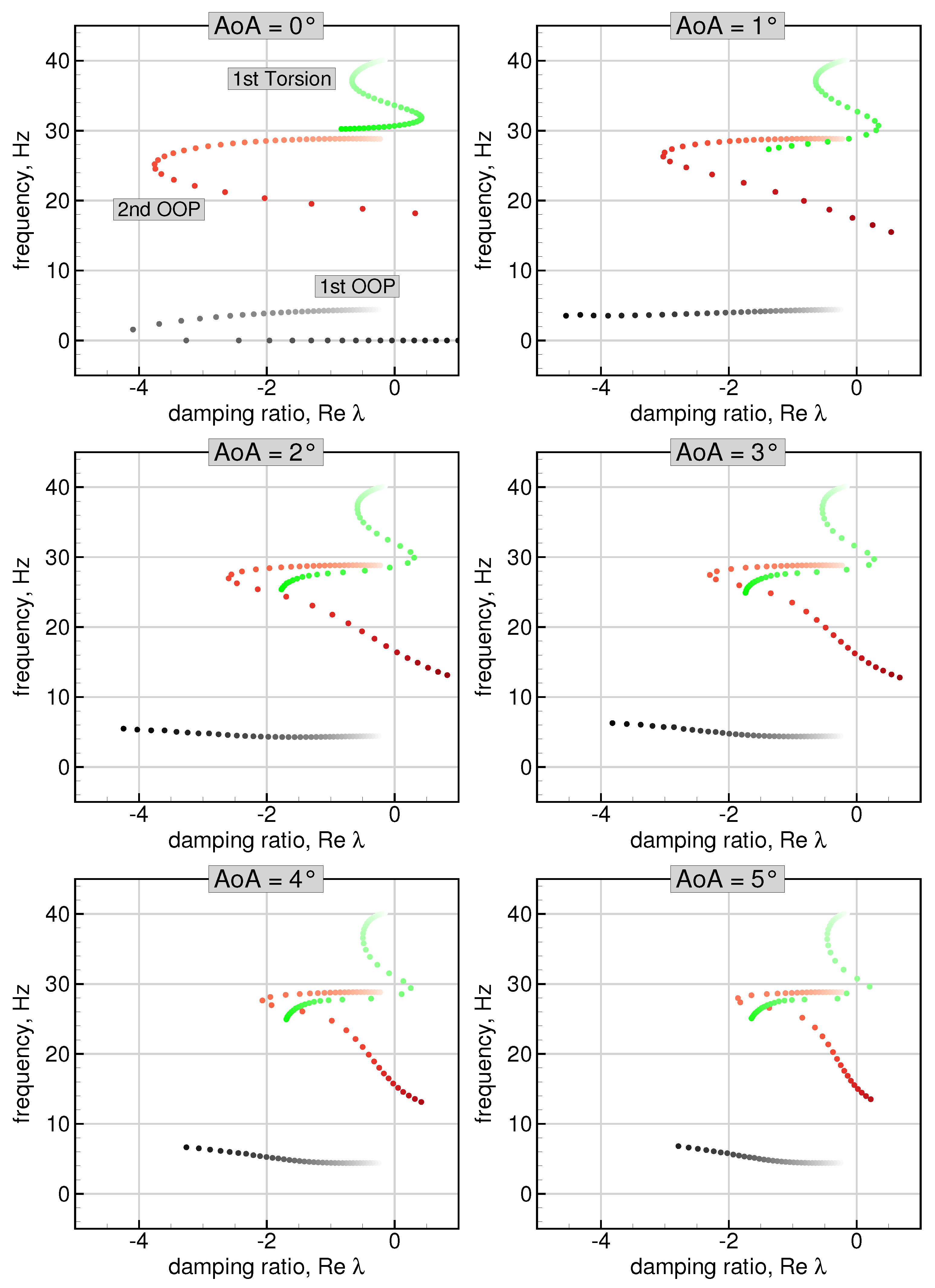
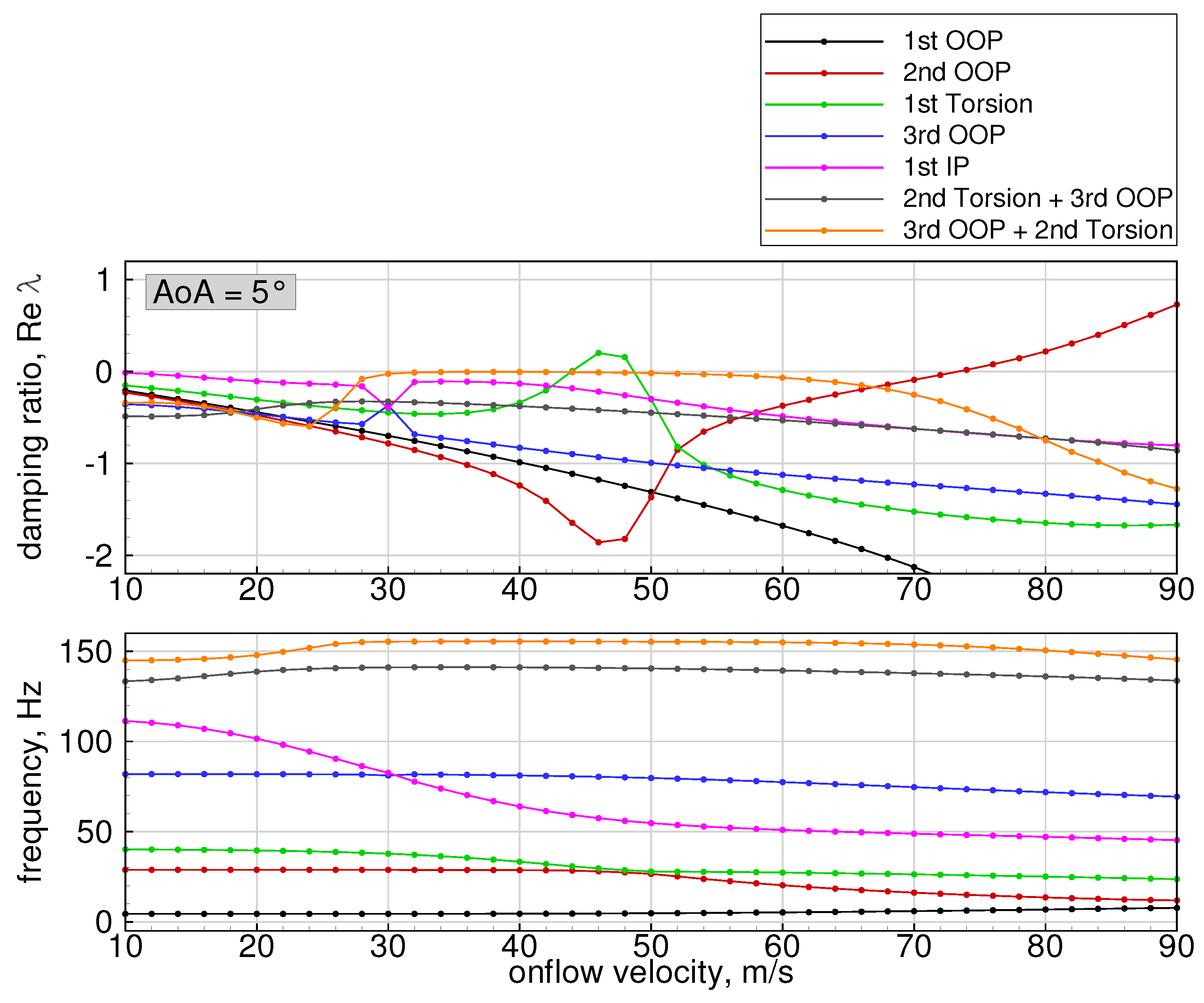
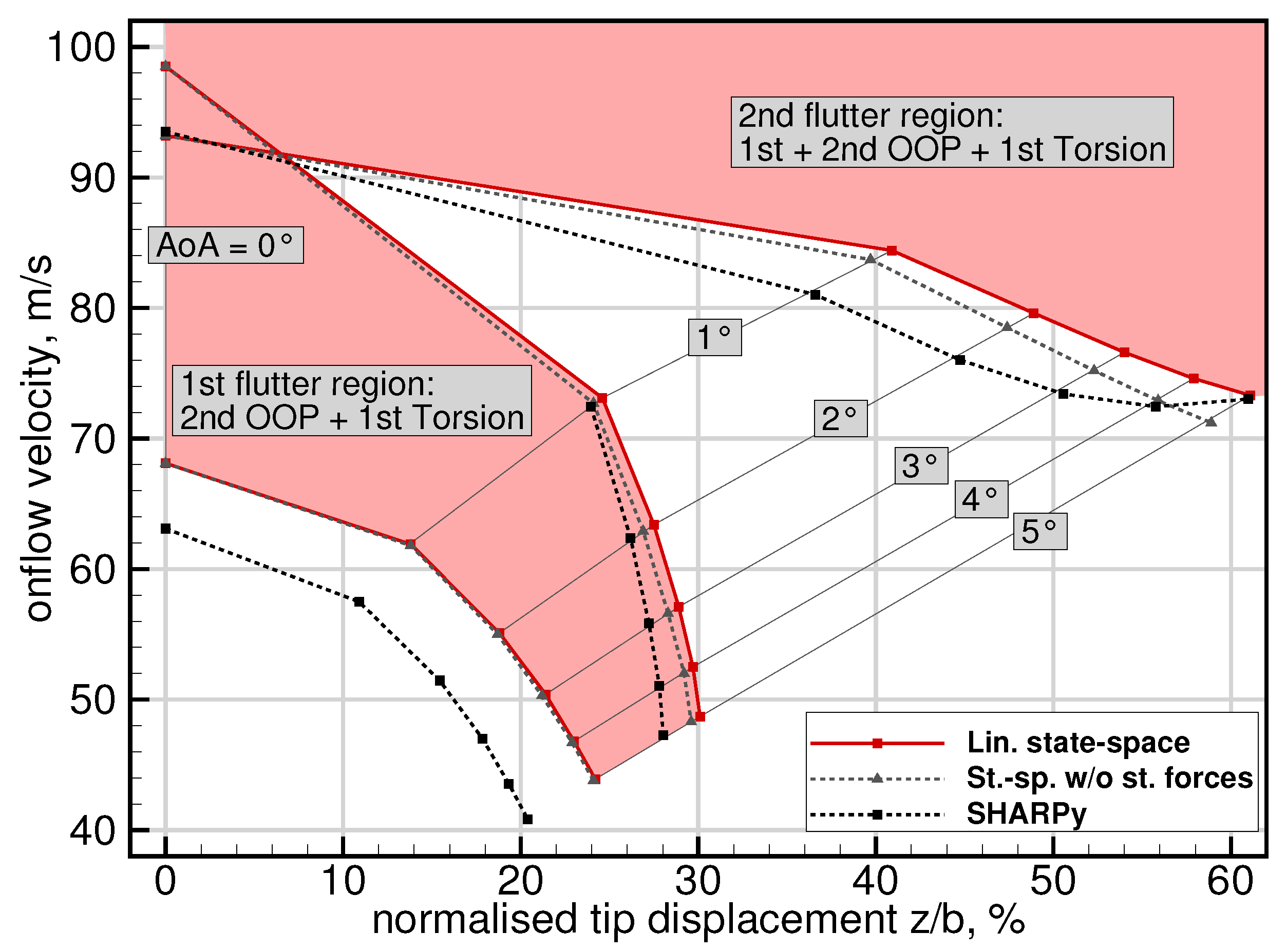
3.3. Stability Analysis Results

Following the investigation of the modal properties as a function of the elastic deformation, the aeroelastic stability of the Pazy wing is analysed by means of the method presented in Section 2.3. The resulting complex eigenvalues are filtered to extract the relevant eigenvalues of the structural states, i.e., the generalised coordinates q 1 , i . In general, the entire solution sequence, including the static coupling solution, is performed for increasing velocities at constant angles of attack. For the stability analysis results presented in this paper, the wake length was set to four times the wing half span and discretised so that the chord of the bound panels equals the chord of the wake panels. With seven modes considered and a discretisation of 16 chordwise and 32 spanwise bound panels for the wing, the system comprises 11,292 states. Once the simulations for the velocity sweep of a specific angle of attack have been completed, there are various ways to illustrate the eigenvalues and the aeroelastic stability of the wing. In the following, both root locus and V-g and V- ω plots are used to depict the behaviour of the wing as a function of the onflow velocity.
The root loci of the Pazy wing for angles of attack ranging from 0 to 5 degrees are depicted in Figure 10. In this case, the evolution of the 1st OOP and 2nd OOP bending mode and the 1st Torsion mode are presented, as only these modes show changes relevant to the stability. The velocity was varied from 10 to 120 m/s for the 0-degree AoA case and from 10 to 90 m/s for all other cases, due to partial convergence issues of the static coupling solver at very large deflections of the wing. An increasing flow velocity corresponds to a higher contrast of the dots, where the step size is set to 2 m/s. It can be seen that the frequency and damping of all three modes considered change significantly when the velocity is increased. Positive real parts, which indicate an instability of the aeroelastic system, are observed in the 1st Torsion and the 2nd OOP bending mode for all AoAs. Comparing the root loci for increasing angles of attack, significant changes in the evolution of the eigenvalues are observed. The instabilities in the 1st Torsion and the 2nd OOP bending mode seem to occur at lower velocities. In contrast, no instabilities are detected in the 1st OOP bending mode, which is mainly due to the smaller velocity range considered.
A more detailed insight into the flutter mechanisms involved is provided by the V-g and V- ω plots. Here, the damping ratio and the frequency of each mode considered are presented with respect to the onflow velocity. For simplification, in the following, the trends of the different modes are identified by the dominant structural mode at low velocities. The plots for the undeformed wing at 0-degree angle of attack and 10 to 120 m/s onflow velocity are shown in Figure 11. In this case, the critical flutter mode is obviously the 1st Torsion mode, which becomes unstable at approximately 68 m/s due to coupling of the 1st Torsion and the 2nd OOP bending mode. As the 1st Torsion mode becomes stable again at 98 m/s, it is referred to as a so-called hump mode [31]. Due to the soft flutter of the 1st Torsion mode with comparatively small positive damping values, this instability might result in a limit cycle oscillation (LCO). An investigation of LCOs by extension of the developed state-space model should therefore be considered for future research. The 2nd OOP bending mode shows instability already at 94 m/s, although its frequency diverges from the frequency of the 1st Torsion mode. This is followed by the flutter onset of the 1st OOP bending mode at 98 m/s. Interestingly, the frequency of this mode reaches a value of 0 Hz at 78 m/s and remains constant, representing a non-oscillatory eigenvalue and thus a steady divergent mode. Since the linearised model only considers the steady induced drag forces at static aeroelastic equilibrium, the 1st IP bending mode exhibits damping values close to zero for the undeformed case.
In contrast, the frequency and damping trends change significantly when the stability analysis is performed for increasing AoAs, e.g., for 5 degrees angle of attack depicted in Figure 12. The flutter onset of the 1st Torsion mode is reduced to approximately 44 m/s, and the mode turns stable again at 48.7 m/s. In comparison to the undeformed case, the velocity range for the instability of this hump mode is also reduced from 30 m/s (0 AoA) to 4.7 m/s. A decrease in flutter velocity is also observed for the 2nd OOP bending mode, which shows instability above 74 m/s. An interesting behaviour is shown by the seventh mode, that incorporates 3rd OOP bending and 2nd Torsion. This mode is only minimally damped at velocities above 30 m/s, which might be caused by the torsional motion included in the pure structural mode shape. Besides the flutter velocities, the complex flutter mode shapes also change as the structure deforms. This can be seen in Figure 13, where the contributions of the pure structural modes to the complex aeroelastic modes—obtained from the eigenvectors of the corresponding eigenvalues and normalised to unit value—are plotted for the undeformed (AoA = 0 ) and the deformed case (AoA = 5 ). For both unstable modes, the contribution of the 1st Torsion at flutter onset increases between 0 and 5 degrees angle of attack. Instead, the magnitude of 1st OOP bending (first flutter onset) and 2nd OOP bending (second flutter onset), respectively, is decreasing.
In general, the decrease in the flutter velocities can be clearly related to the change of the structural eigenvalues due to the deflection of the wing (cf. Section 3.2). The effect of these structural nonlinearities becomes more apparent in Figure 14, in which the flutter velocity is plotted as a function of the normalised tip displacement for six different angles of attack. As already expected and observed in the damping trends, an increase in angle of attack results in a significant reduction in the flutter velocity of both critical flutter modes. The diagram also illustrates that the region of instability of the hump mode becomes smaller with increasing angle of attack. In addition, the velocity range between the first and the second flutter mode is considerably increasing. The phenomenon of a restricting maximum tip deflection at high angles of attack appears in the ’stabilisation’ velocity of the hump mode, which is limited to approximately 30%. This is clearly a consequence of the change of modal properties (only due to the deflection of the wing) discussed in the previous section as the frequency of the structural 1st Torsion mode approaches the frequency of the 2nd OOP bending mode at approximately 31% (see Figure 9).
Similar to the results of the static coupling simulations, the results of the stability analysis are also compared to numerical data obtained from SHARPy at Imperial College. Considering the undeformed case, high deviations in the velocity of the first flutter onset are observed, while the velocity of the second flutter onset shows a good match. As the results of the stability analysis for the undeformed wing were validated with results obtained by Nastran SOL145 (see [25]) using the same full FE model, a possible explanation for the deviations could be the different solution approaches (beam vs. full FE model). With increasing angle of attack, the results become additionally influenced by the differences in the static coupling results, as indicated by the deviations of the flutter points in the x axis (normalised tip displacement). Overall, the development of the flutter velocities as a function of the tip displacement shows qualitatively similar behaviour for both solutions. Interestingly, the effect of the steady aerodynamic loads seems to affect the stability of the system only at higher velocities. While only small differences are observed for the first flutter onset and offset, the velocity for the second flutter mode is slightly underestimated when the steady forces at aeroelastic equilibrium are not considered in the stability analysis ( Γ w 0 = 0 ).

4. Conclusions

This paper presented static coupling and stability analysis results for the Pazy wing aeroelastic benchmark investigated by the Large Deflection Working Group within the Third Aeroelastic Prediction Workshop. An aeroelastic solver developed at DLR was used for the numerical simulations, coupling a geometrically nonlinear vortex lattice method with the finite element solver Nastran. Follower forces as well as geometric nonlinearities were considered by a fully nonlinear formulation of the aerodynamic solution (deformed aerodynamic grid, update of panel normals, etc.) and by using the nonlinear solution sequence SOL400 in Nastran for the structural solution. For the stability analysis, the aeroelastic system was linearised at static equilibrium points with large deformations. A linear aerodynamic model was derived analytically at first by transforming the existing unsteady vortex lattice implementation into a linear discrete-time state-space system, using the circulation of the wake panels as system states. From a structural point of view, a modal approach in generalised coordinates was used and likewise converted into a linear discrete-time state-space model. Both models were integrated into a monolithic aeroelastic state-space model, which accounts for the deformed aerodynamic grid, the steady aerodynamic loads at aeroelastic equilibrium and the changed natural modes (pre-loaded structural eigenvalue analysis) due to the deflection of the structure. The aeroelastic stability is determined by solving the homogeneous eigenvalue problem for the dynamics matrix of the system.
The results of static coupling simulations were presented for a range of different AoAs and velocities, reaching a maximum of 47% tip displacement for the highest AoA and onflow velocity. Comparatively small deviations were observed when the results were compared to data obtained by another member of the LDWG. Regarding the influence of the geometric nonlinearities on the structural properties, significant changes appeared mainly in the frequencies and the eigenvectors of two structural modes. These changes of the modal properties were found to have a major influence on the aeroelastic stability, as the flutter onset velocities of the first two instabilities are clearly reduced with increasing angle of attack. Comparison of the stability analysis results with data obtained from a similar solution method using an equivalent beam model revealed larger differences, especially for the velocity of the first flutter onset.
The goal of validating the simulation results with experimental data has not yet been achieved but will therefore have high priority in the future. In addition, it seems reasonable to investigate how the skin and its prestressing could actually be included in the structural model, since all simulations presented in this work were performed using the model without skin. Another aspect for future research should be an extension of the proposed state-space formulation in order to investigate limit cycle oscillations which occurred at large deformations during the wind tunnel tests. As the solution of the eigenvalue problem becomes computationally demanding due to the large number of aerodynamic states, the application of model order reduction methods (e.g., balanced truncation) to the linearised aerodynamic model seems favourable in order to save computational costs and to speed up the stability analysis.

Author Contributions

Conceptualisation, M.R.R.; methodology, M.R.R. and J.H.; software, M.R.R. and J.H.; validation, J.H.; formal analysis, J.H.; investigation, M.R.R. and J.H.; resources, M.R.R.; data curation, J.H.; writing—original draft preparation, J.H.; writing—review and editing, M.R.R.; visualisation, J.H.; supervision, M.R.R. All authors have read and agreed to the published version of the manuscript.

Funding

This research received no external funding.

Institutional Review Board Statement

Not applicable.

Informed Consent Statement

Not applicable.

Data Availability Statement

The data presented in this study as well as the CAD and FE models of the Pazy wing are so far available on request from the corresponding author (see the AePW3 website [12]). The results from the Imperial College Group and others are publicly available in Zenodo at https://doi.org/10.5281/zenodo.4311606 (accessed on 28 August 2021).

Acknowledgments

The authors would like to thank the Imperial College group for sharing computational results. In addition, the authors would like to acknowledge the colleagues from Technion for providing simulation models and experimental data. The support of the DLR Institute of Aeroelasticity is also acknowledged.

Conflicts of Interest

The authors declare no conflict of interest.

Abbreviations

The following abbreviations are used in this manuscript:
Acronyms
AePW3Third Aeroelastic Prediction Workshop
CFDComputational Fluid Dynamics
DLRGerman Aerospace Center
DOFDegree of Freedom
FEFinite Element
FSIFluid Structure Interaction
IPIn-plane
LCOLimit Cycle Oscillation
LDWGLarge Deflection Working Group
OOPOut-of-plane
SHARPySimulation of High-Aspect Ratio aeroplanes in Python
VLMVortex Lattice Method
Nomenclature
A p Area of aerodynamic panel
bWing span
zEigenvalue of discrete-time state-space system
Δ t Time step size
λ Eigenvalue of continuous-time state-space system
ρ Fluid density
ω Natural frequency
ϕ Velocity potential
A Dynamics matrix
AIC Aerodynamic influence coefficients matrix
B Control/Input matrix
C Sensor/Output matrix
D Direct term/Feed-through matrix
F Force vector of aerodynamic panel
f Generalised forces vector
H Coupling matrix
I Identity matrix
M Shifting matrix for wake-shedding process; Interpolation matrix
n Normal vector of aerodynamic panel
q Vector of generalised coordinates
r Quarter chord line vector of aerodynamic panel
RHS Vector of kinematic boundary conditions at collocation points of aerodynamic panels
u Input vector
V Velocity vector of aerodynamic panel
WIC Wake influence coefficients matrix
x State vector
y Output vector
Γ Vector of circulations of aerodynamic panels
Φ Eigenvectors of structural modes
Indices
Aaerodynamic
bbound
cw.r.t. collocation point
ddisplacement transfer; induced drag component
e f f effective
e l elastic
fforce transfer
ndiscrete time step
qw.r.t. quarter point
r b rigid body
ssteady component
Sstructural
uunsteady component
wwake
0conditions at static aeroelastic equilibrium
˜ equivalent matrix of a vector in blockwise diagonal form
˙ first time derivative

References

  1. Ritter, M.; Dillinger, J.; Meddaikar, Y.M. Static and dynamic aeroelastic validation of a flexible forward swept composite wing. In Proceedings of the 58th AIAA/ASCE/AHS/ASC Structures, Structural Dynamics, and Materials Conference, Grapevine, TX, USA, 9–13 January 2017. [Google Scholar]
  2. Avin, O.; Drachinsky, A.; Ben-Shmuel, Y.; Raveh, D. Design of an experimental benchmark of a highly flexible wing. In Proceedings of the 60th Israel Annual Conference on Aerospace Sciences, Tel Aviv/Haifa, Israel, 4–5 March 2020. [Google Scholar]
  3. Zimmer, M. Integral design and optimisation process for a highly flexible generic long range jet transport with flight mechanic derivative constraints. In Proceedings of the AIAA Scitech 2021 Forum, Reston, VA, USA, 11–21 January 2021. [Google Scholar]
  4. Ritter, M.; Hilger, J.; Zimmer, M. Static and dynamic simulations of the Pazy wing aeroelastic benchmark by nonlinear potential aerodynamics and detailed FE model. In Proceedings of the AIAA Scitech 2021 Forum, Reston, VA, USA, 11–21 January 2021. [Google Scholar]
  5. Cesnik, C.E.; Senatore, P.J.; Su, W.; Atkins, E.M.; Shearer, C.M. X-HALE: A Very Flexible Unmanned Aerial Vehicle for Nonlinear Aeroelastic Tests. AIAA J. 2012, 50, 2820–2833. [Google Scholar] [CrossRef] [Green Version]
  6. Ritter, M. An Extended Modal Approach for Nonlinear Aeroelastic Simulations of Highly Flexible Aircraft Structures. Ph.D. Thesis, TU Berlin, Berlin, Germany, 2018. [Google Scholar]
  7. Noll, T.E.; Brown, J.M.; Perez-Davis, M.E.; Ishmael, S.D.; Tiffany, G.C.; Gaier, M. Investigation of the Helios Prototype Aircraft Mishap: Volume I Mishap Report; NASA Langley Research Center: Hampton, VA, USA, 2001. [Google Scholar]
  8. Cea, A.; Palacios, R. Nonlinear modal aeroelastic analysis from large industrial-scale models. In Proceedings of the AIAA Scitech 2019 Forum, San Diego, CA, USA, 7–11 January 2019. [Google Scholar]
  9. Ritter, M.; Cesnik, C.E.; Krüger, W.R. An enhanced modal approach for large deformation modeling of wing-like structures. In Proceedings of the 56th AIAA/ASCE/AHS/ASC Structures, Structural Dynamics, and Materials Conference, Kissimmee, FL, USA, 5–9 January 2015. [Google Scholar]
  10. Tang, D.; Dowell, E.H. Experimental and Theoretical Study on Aeroelastic Response of High-Aspect-Ratio Wings. AIAA J. 2001, 39, 1430–1441. [Google Scholar] [CrossRef]
  11. Xie, C.; Liu, Y.; Yang, C.; Cooper, J.E. Geometrically Nonlinear Aeroelastic Stability Analysis and Wind Tunnel Test Validation of a Very Flexible Wing. Shock Vib. 2016, 2016, 5090719. [Google Scholar] [CrossRef]
  12. AePW-3 Overview. Available online: https://nescacademy.nasa.gov/workshops/AePW3/public/ (accessed on 20 July 2021).
  13. Ritter, M.; Neumann, J.; Krüger, W.R. Aeroelastic Simulations of High Reynolds Number Aero Structural Dynamics Wind Tunnel Model. AIAA J. 2016, 54, 1962–1973. [Google Scholar] [CrossRef]
  14. Ritter, M.; Jones, J.; Cesnik, C.E. Free-flight Nonlinear Aeroelastic Simulations of the X-HALE UAV by an Extended Modal Approach. In Proceedings of the International Forum on Aeroelasticity and Structural Dynamics, Como, Italy, 25–28 June 2017. [Google Scholar]
  15. Palacios, R.; Murua, J.; Cook, R. Structural and Aerodynamic Models in Nonlinear Flight Dynamics of Very Flexible Aircraft. AIAA J. 2010, 48, 2648–2659. [Google Scholar] [CrossRef] [Green Version]
  16. Palacios, R. Nonlinear normal modes in an intrinsic theory of anisotropic beams. J. Sound Vib. 2011, 8, 1772–1792. [Google Scholar] [CrossRef] [Green Version]
  17. Shearer, C.M.; Cesnik, C.E. Nonlinear Flight Dynamics of Very Flexible Aircraft. J. Aircr. 2007, 44, 1528–1545. [Google Scholar] [CrossRef] [Green Version]
  18. Jones, J.; Cesnik, C.E. Nonlinear Aeroelastic Analysis of the X-56 Multi-Utility Aeroelastic Demonstrator. In Proceedings of the AIAA Scitech Forum, 15th Dynamics Specialists Conference, San Diego, CA, USA, 4–8 January 2016. [Google Scholar]
  19. Bathe, K.J. Finite Element Procedures, 2nd ed.; Klaus-Jürgen Bathe: Watertown, MA, USA, 2008. [Google Scholar]
  20. MSC Software. MSC Nastran 2017: Nonlinear User’s Guide SOL 400; MacNeal-Schwendler Corporation: Newport Beach, CA, USA, 2016. [Google Scholar]
  21. Murua, J.; Palacios, R.; Graham, J.M.R. Applications of the unsteady vortex-lattice method in aircraft aeroelasticity and flight dynamics. Prog. Aerosp. Sci. 2012, 55, 46–72. [Google Scholar] [CrossRef] [Green Version]
  22. Katz, J.; Plotkin, A. Low Speed Aerodynamics, 2nd ed.; Cambridge Aerospace Series; Cambridge University Press: Cambridge, UK, 2001; Volume 13. [Google Scholar]
  23. Mauermann, T. Flexible Aircraft Modelling for Flight Loads Analysis of Wake Vortex Encounters. Ph.D. Thesis, TU Braunschweig, Braunschweig, Germany, 2010. [Google Scholar]
  24. Beckert, A.; Wendland, H. Multivariate interpolation for fluid-structure-interaction problems using radial basis functions. Aerosp. Sci. Technol. 2001, 5, 125–134. [Google Scholar] [CrossRef]
  25. Hilger, J. Nonlinear Aeroelastic Simulations and Stability Analysis of a Highly Flexible Wing. Master’s Thesis, Hamburg University of Applied Sciences, Hamburg, Germany, 2021. [Google Scholar]
  26. Murua, J.; Martínez, P.; Climent, H.; van Zyl, L.; Palacios, R. T-tail flutter: Potential-flow modelling, experimental validation and flight tests. Prog. Aerosp. Sci. 2014, 71, 54–184. [Google Scholar] [CrossRef]
  27. Åström, K.J.; Murray, R.M. Feedback Systems: An Introduction for Scientists and Engineers; Princeton University Press: Princeton, NJ, USA, 2008. [Google Scholar]
  28. Avin, O.; Raveh, D.E.; Drachinsky, A.; Ben-Shmuel, Y. An experimental benchmark of a very flexible wing. In Proceedings of the AIAA Scitech 2021 Forum, Reston, VA, USA, 11–21 January 2021. [Google Scholar]
  29. Goizueta, N.; Drachinsky, A.; Wynn, A.; Raveh, D.E.; Palacios, R. Flutter predictions for very flexible wing wind tunnel test. In Proceedings of the AIAA Scitech 2021 Forum, Reston, VA, USA, 11–21 January 2021. [Google Scholar]
  30. del Carre, A.; Muñoz-Simón, A.; Goizueta, N.; Palacios, R. SHARPy: A dynamic aeroelastic simulation toolbox for very flexible aircraft and wind turbines. J. Open Source Softw. 2019, 4, 1885. [Google Scholar] [CrossRef] [Green Version]
  31. Norton, W.J. Structures Flight Test Handbook; Air Force Flight Test Center: Edwards Air Force Base, CA, USA, 1990. [Google Scholar]
Figure 1. Comparison of results obtained by nonlinear modal solver and linear aeroelastic state-space model for Pazy wing structural model with V = 50 m/s, q 1 , i 0 = 0.001.
Aerospace 08 00308 g001aAerospace 08 00308 g001b
Figure 2. Steady iterative coupling solution sequence including Nastran nonlinear static solution.
Aerospace 08 00308 g002
Figure 3. Linearised static coupling solution sequence including a time-marching procedure (optional) and the stability analysis.
Aerospace 08 00308 g003
Figure 4. The (Pre)-Pazy wing wind tunnel model (Reproduced with permission from Drachinsky [2]; published by IACAS, 2020).
Aerospace 08 00308 g004
Figure 5. Nastran FE model of the Pazy wing composed by beam and shell elements representing the main aluminum spar and the 3D printed chassis; model without Oralight skin.
Aerospace 08 00308 g005
Figure 6. VL grid, coupling nodes of the FE model selected for the transfer of forces/displacements and 33 equidistant points used for the evaluation of deflections.
Aerospace 08 00308 g006
Figure 7. Results of static coupling simulations for 30 m/s onflow velocity evaluated at 44.75% chord.
Aerospace 08 00308 g007
Figure 8. Comparison of static coupling results with data provided by Imperial College (SHARPy) for 50 m/s onflow velocity evaluated at 44.75% chord.
Aerospace 08 00308 g008
Figure 9. Evolution of the eigenfrequencies of the Pazy wing as function of the deformation for two different angles of attack.
Aerospace 08 00308 g009
Figure 10. Root loci of the Pazy wing for AoAs ranging from 0 to 5 degrees and velocities from 10 to 120/90 m/s; increased contrast corresponds to higher flow velocity.
Aerospace 08 00308 g010
Figure 11. Damping and frequency trends of the Pazy wing for 0 degrees angle of attack and velocities ranging from 10 to 120 m/s.
Aerospace 08 00308 g011
Figure 12. Damping and frequency trends of the Pazy wing for 5 degrees angle of attack and velocities ranging from 10 to 90 m/s.
Aerospace 08 00308 g012
Figure 13. Contributions of the structural DOFs to the unstable complex mode shapes of the Pazy wing for 0 and 5 degrees angle of attack and velocities ranging from 10 to 120/90 m/s; vertical line marks flutter onset.
Aerospace 08 00308 g013
Figure 14. Regions and boundaries of flutter instabilities of the Pazy wing for AoAs ranging from 0 to 5 degrees.
Aerospace 08 00308 g014
Table 1. Properties of the Pazy wing (data from [2]).
PropertyMeasurement
Span550 mm
Chord100 mm
Area0.055 m2
Main spar550 × 60 × 2.5 mm
Aspect ratio5.5
AirfoilNACA 0018
Mass0.321 kg
Table 2. Parameters of the static coupling simulation setup.
Angle of attack1–10°
Free stream velocity30, 40, 50 m/s
Density1.225 kg/m3
Chordwise panels16
Spanwise panels32
Wake length2000 m
Gravityon (z direction)
Table 3. Comparison of computational and experimental results for wing tip deformation at static aeroelastic equilibrium (data from [28]).
AoAVelocityTip Displacement Experiment (Skin)Tip Displacement Simulation (No Skin) Δ
30 m/s52 mm60 mm15.3%
50 m/s157 mm182 mm15.9%
55 m/s255 mm267 mm4.7%
Publisher’s Note: MDPI stays neutral with regard to jurisdictional claims in published maps and institutional affiliations.

