Article

Model Updating and Aeroelastic Correlation of a Scaled Wind Tunnel Model for Active Flutter Suppression Test

Department of Aerospace Science and Technology, Politecnico di Milano, Via La Masa 34, 20156 Milano, Italy
*
Author to whom correspondence should be addressed.
Aerospace 2021, 8(11), 334; https://doi.org/10.3390/aerospace8110334
Submission received: 5 July 2021 / Revised: 30 October 2021 / Accepted: 1 November 2021 / Published: 7 November 2021
(This article belongs to the Special Issue Aeroelasticity, Volume III)

Abstract

:
This article presents a modal correlation and update carried out on an aeroelastic wind tunnel demonstrator representing a conventional passenger transport aircraft. The aim of this work is the setup of a corresponding numerical model that is able to capture the flutter characteristics of a scaled aeroelastic model designed to investigate and experimentally validate active flutter suppression technologies. The work described in this paper includes different finite element modeling strategies, the results of the ground vibration test, and finally the strategies adopted for modal updating. The result of the activities is a three-dimensional hybrid finite element model that is well representative of the actual aeroelastic behavior identified during the wind tunnel test campaign and that is capable of predicting the flutter boundary with an error of 1.2%. This model will be used to develop active flutter suppression controllers, as well as to perform the sensitivity analyses necessary to investigate their robustness.

1. Introduction

The use of scaled wind tunnel models to validate simulation results is well known in the field of aeroelastic predictions for both military and civil transport aircraft. The activity is not limited to the research investigations phase but can also support and mitigate the risk of the certification phase based on full-scale flight tests. This is particularly true in the case of unconventional configurations whose aeroelastic behavior is more difficult to predict. The scaling process, as well as the adopted strategies to realize aeroelastically scaled wind tunnel models, has been completely described by Bisplinghoff in [1]. The traditional approach is typically based on a condensation of the mass and stiffness distributions of the considered aircraft to those of beams representing the elements of the model with attached masses and separated aerodynamic sectors that do not appreciably contribute to the overall bending or torsional stiffness. Thus, the entire process is mainly reduced to the definition of the properties of the scaled beam-like structures to match the actual (scaled) stiffness distribution of the reference aircraft well. It is clear that, with this approach, the actual structural topology of the aircraft is not reproduced, and the final configuration of the scaled model is mainly driven by the manufacturing technologies, by the material properties, and by the need to install the sensors and actuators necessary to investigate the relevant aeroelastic phenomena.
The current tendency for modern aircraft to show enhanced flexibility, as well as to enable aeroelastic deflections to be used in a beneficial manner [2], makes the use of scaled aeroelastic wind tunnel models more important. On the other side, the adoption of more and more complex Active Control (AC) systems for aeroelastic control, together with the need to validate their performances during the wind tunnel test campaign, opens the door to new manufacturing technologies, such as 3D printing and alternative materials [3], but at the same time makes the level of aeroelastic correlation between the scaled model and the reference aircraft even more important. This is the case for the example of flutter [1], which is a dynamic instability that results from the coupling of aerodynamics and structural dynamics. It represents a complex phenomenon and, at the same time, a design constraint that is complicated due to its dependence on the coupling of close structural modes, and thus the mass and stiffness distributions within the structure. The level of representativity of the scaled model becomes a key factor, especially in the case where not only the phenomenon but also its active control is under investigation. The current advanced state of the art of AC sees Active Flutter Suppression systems as the main solution to this kind of instability [4]. Since flutter is an aggressive and abrupt kind of instability, it is urgent to figure out how precise and robust the AC law has to be. Its design and implementation rely strongly on the accuracy of the model representing the real behavior of the aircraft.
In this broad context, the activities described herein fit the development of a well-correlated mathematical model that is able to fully characterize the phenomenon and that can be used as the basis for the design of control laws. As noted in [4], the move from theoretical–numerical studies or studies based on highly simplified wind tunnels or flight models to the full implementation of the technology requires more experimental work. The investigation should comprehensively consider wind tunnels and in-flight tests, using scaled models that represent real full-size aircraft in terms of their configuration and complexity, as this would help identify technological deficiencies and development needs, especially from the perspective of safety and the associated uncertainty–reliability simulation and the test capabilities required. Many works can be found in the literature on the numerical/experimental correlation of wing structures and updates to airplane models. An interesting work on the aeroelastic scaling and optimization of a joined-wing aircraft is described in [5,6]. Some relevant work with a scope similar to that of this manuscript was carried out during the US-based Performance Adaptive Aeroelastic Wing (PAAW) project [7] and the European Flutter Free Flight Envelope Expansion for Economical Performance improvement (FlexOP) project [8,9,10], while a summary of both projects can be found in [11].
The Department of Aerospace Science and Technology (DAER) at Politecnico di Milano (PoliMi), in collaboration with the University of Washington, contributed to the so-called Active Flutter Suppression (AFS) project that aimed to validate active flutter suppression technologies. On the basis of its large amount of experience during the last 30 years in the design, manufacturing, and testing of wind tunnel aeroelastic models [12,13,14], DAER developed a dedicated wind tunnel model, called X–Dia, to be used for the AFS project and focused on these technologies, including uncertainties and robustness issues [15]. This paper reports the activity required to set up the numerical aeroelastic model and in particular the numerical vs. experimental aeroelastic correlation and updating phase. Traditionally, this activity is formulated as an optimization problem [16]. The state of the art of optimization software is extraordinarily advanced; many commercial optimizers allow very complex problems to be considered, finding the best minimum solution in the infinite set with a user-friendly and automated process. In this case, the design sensitivity and optimization of MSC/NASTRAN has been adopted [17].
The work is set out as follows: Section 2 presents the X–Dia model, in terms of its conceptual design, realization, and testing procedures to characterize its dynamic and aeroelastic behavior. The large experimental campaign has made measures available with which researchers can study the flutter mechanism and tune the mathematical model. Section 3 summarizes the results of the experimental modal analysis activities representing the targets for the updating process. Section 5 describes the process adopted to gain the final FEM model that optimally describes the real structure and its flutter onset, based on experimental data, proper modeling considerations, and the optimization algorithm. This last aspect is deeply considered in Section 6, outlining the general rules, the modeling constraints, and the critical points found in the process of the updating phase. Section 7 contains the comparison results of the modal and flutter analyses between the experimental data and the mathematical model predictions and, in light of the correlation evaluation methods, the necessary steps to achieve the optimum. In particular, through different sub-sections, we provide the evolution of the updating process of the FEM model based on an optimization algorithm to achieve an optimum correlation level and accurately determine the flutter boundary. The procedure stands out in the multi-stage development of the model due to the ever-increasing level of detail and structural interventions according to the aeroelastic response requirements. Finally, Section 8 presents the conclusions on the work that has been carried out and a brief reminder of the obtained results in terms of a comparison between the numerical and experimental flutter velocity.

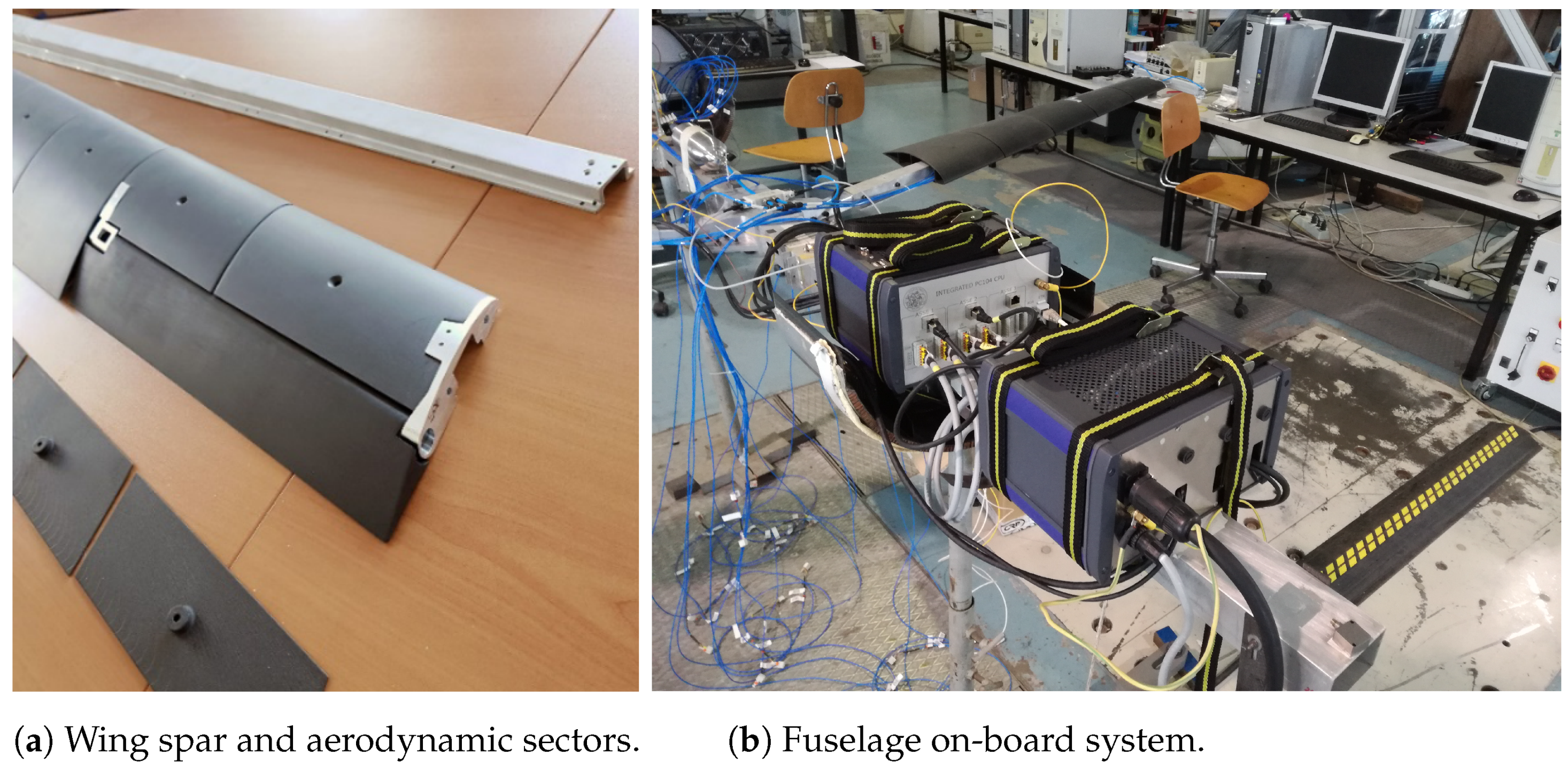
2. The X–Dia Wind Tunnel Model

The X–DIA model was initially conceived by PoliMi to study different topics concerning flight mechanics, aeroelasticity, and active controls. Its configuration was subject to variations according to the intended purpose. The final model shows a more conventional layout, with a low positive swept wing and a T-tail without the presence of the canard, (the original configuration is reported in [12,13], while the final model is shown in Figure 1) to meet the aeroelastic demands of the activities. The model is representative of a generic aircraft, but it is not a scaled version of a specific aircraft. The design specifications were related to a generic configuration and wind tunnel test requirements.
The skeleton of the X–Dia model is composed of aluminum beams connected to each other. The fuselage beam part is in a tubular structure with a rectangular aluminum section. The wing spar is a beam with an omega section shape, while the vertical and horizontal ones are cross-shaped. Connections of structural elements are designed and milled from aluminum blocks. The wing spar is covered with discrete aerodynamic sectors, made by 3D printing technology using Windform composite SLS (Selective Laser Sintering) materials (developed and patented by CRP Technology) to guarantee high stiffness, so to avoid local modes. Both the wing spar and aerodynamic sectors are shown in Figure 2a. They are designed to allow internal space for the installation of the instrumentation. Two milled ribs support the aileron hinges and the servo-actuators, which are based on the Harmonic Drive electric motors (RSF-5B) coupled with an in-house developed servo-control law [18].
X–Dia is equipped with an on-board computer to manage the active control systems and data acquisitions. The embedded computer is equipped with an in-house developed Real Time Application Interface (RTAI), a real-time operating system based on Linux. The embedded computers, as well all the necessary acquisition cards, are based on the PC-104 form factor allowing for a small final size and weight of the complete embedded system, which is shown in Figure 2b. The main sensors are MEMS accelerometers by PCB, which were selected for their high accuracy at low frequencies and mainly because of being already pre-amplified. The corresponding channels could be read by a standard data acquisition system without the need of expensive and heavy IEPE modules, usually adopted in case of piezo-electric accelerometers. This choice allowed for a small embedded computer to be installed inside the model that is capable of managing the test in terms of acquisition and active control duties. By having the complete instrumentation on-board, the model is almost in a free–free condition inside of the wind tunnel, which is a beneficial circumstance for this kind of test since a wind tunnel is by definition a noisy environment.
Among the latest changes made to the new X–Dia model is that a safety device was installed at the tips of the wing, as shown in Figure 3, in view of the flutter wind tunnel tests. This system allows us to change the mass configuration so to eliminate the flutter instability. The device contains a small mass of 200 gr able to slide inside a pod from two on–off positions (respectively forward and backward) thanks to a linear pneumatic actuator. The slider length is about 15 cm. According to the position of the sliding mass, the aircraft is prone to flutter or not. The forward mass position has been designed to increase the flutter velocity above the maximum velocity obtainable in the wind tunnel. During the flutter wind tunnel tests, the mass is positioned in the backward position. Then, the maximum vertical acceleration of the tip is monitored. When a threshold value is exceeded the system is automatically switched on to move the mass in the forward position in both pods to immediately stop the flutter and to avoid damaging the model. The threshold value has been setup during the preliminary tests to 4g, a value found to be the best compromise to see a complete flutter development without reaching dangerous vibration levels.
The tip sensors data are processed separately, so that the left and right safety pods can work independently as they are activated only by local acceleration, practically developing two independent co-located anti-flutter devices. This strategy offers the possibility to face the onset of several kinds of flutter (symmetric, non-symmetric, body-freedom flutter, etc.).
During the wind tunnel test, carried out at PoliMi’s Large Wind Tunnel, the aircraft is free–free suspended in the wind tunnel by means of an elastic connection made by cables so that the structure can experience the rigid body modes with a frequency less than 1 Hz.

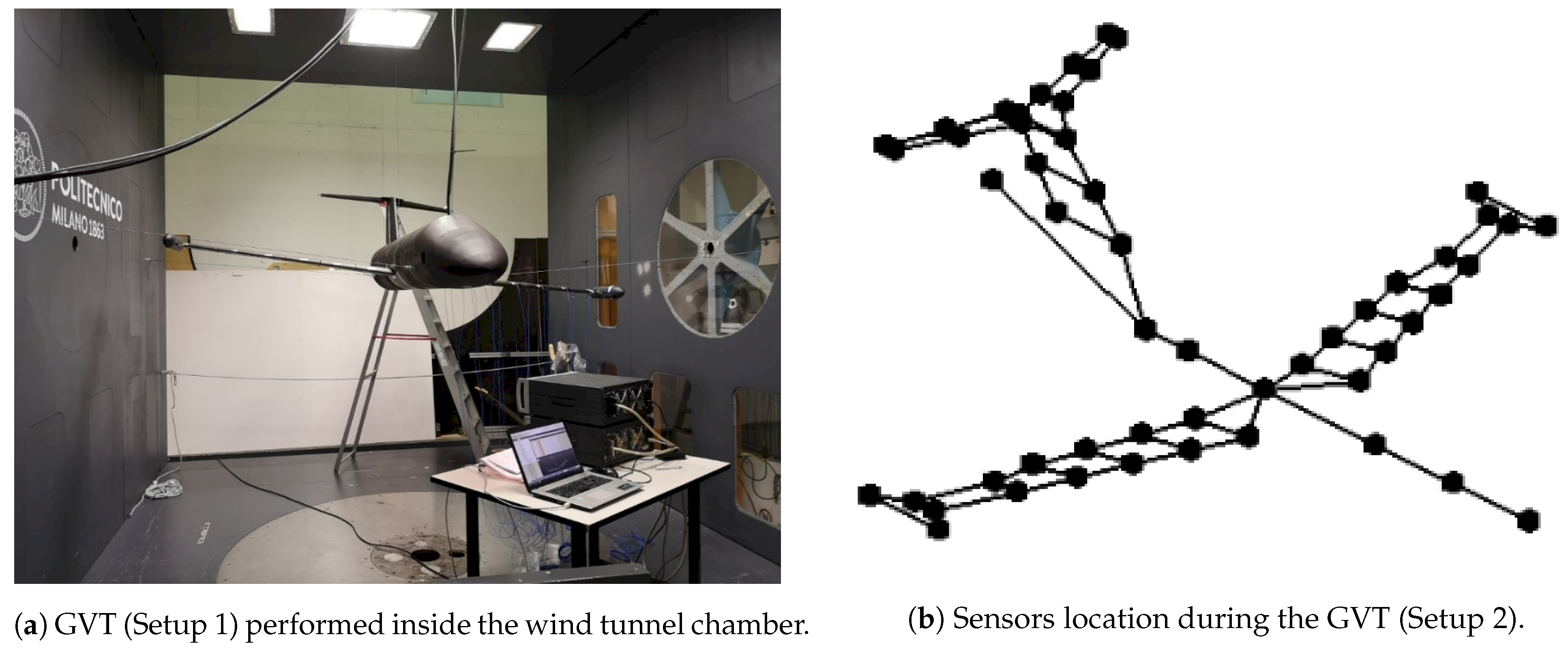
3. Ground Vibration Test (GVT)

The experimental campaign had a double purpose: identify the actual dynamic properties of the model as well identify the flutter mechanism. The first target has been achieved by a dedicated Ground Vibration Test (GVT) session [19,20,21]. With the evolution of the project, the mass and in some cases the stiffness distribution of the model changed due to the installation of different components. In particular, the following items have impacted the dynamic properties of the model: the installation of reinforcing rods to increase the stiffness out of plane of the original horizontal tail; the on-board data acquisition system, which heavily influences the model mass and CG position;and the flutter stopper safety devices that were installed on both the wing tips. Different GVT sessions have been carried out for tracking the linear dynamic properties and for periodically updating the intermediate numerical models adopted [19,20,21]. The two most relevant configurations in view of numerical vs. experimental correlation and model updating were selected, with the anti-flutter safety device installed on both the wing tips and the moving mass in rear position or in forward position. For these configurations, two different sensors setup have been adopted:
Setup 1:
all the lifting surfaces—i.e., wings, horizontal planes, and vertical tail—have been measured in the out-of-plane direction. A roving hammer impact test has been carried out, limiting the mass loading effect due to the mass of the accelerometers. Five fixed accelerometers have been installed upon the structure and used as references, while the other points have been used for excitation and computed with 10 averages, for a total of 46 measurements.
Setup 2:
the left wing has been instrumented with 28 fixed accelerometers that are equally distributed to measure in both in and out-of-plane direction. The excitation has been introduced by the hammer impact. This setup has been realized mainly to investigate deeply specific aspects, such as the dynamic behavior of the pod.
Two mass configurations have been considered, depending on the anti-flutter safety device:
1.
Safety On: the aircraft with the mass of both anti-flutter devices fully forward.
2.
Safety Off: the aircraft with the mass of both anti-flutter devices fully backward.
The aeroelastic demonstrator inside the wind tunnel chamber during the GVT is shown in Figure 4a, while the detailed experimental mesh adopted for the Setup 1 is shown in Figure 4b. A database of Frequency Response Functions (FRFs) has been acquired considering a sampling frequency of 512 Hz and a frequency resolution of 0.0625 Hz, while the anti-aliasing filters cut frequency is 80% of the Nyquist frequency, which is set to 200 Hz. The FRFs have been computed using the H v method to eliminate the influence of uncorrelated noise in the input and the output signals [22]. The wind tunnel configuration adopted during the GVTs is the same one used during the flutter tests, to reduce as much as possible the differences in the dynamic behavior of the model due to the suspension system.
Once the measurements were collected, a preliminary validation phase was planned to substantiate the quality of the measurements. Although many verification criteria are available in the literature [23], the Modal Assurance Criterion (MAC) was chosen [24]. The experimental validation was completed using Modal Phase Collinearity (MPC), Mean Phase Deviation (MPD), and Mode Overcomplexity Value (MOV) indexes.
Table 1 and Table 2 show the comparison among frequencies and damping measured with the tip masses in forward and rear positions, respectively. Figure 5 shows the comparison between measured mode shapes with tip masses in forward and rear positions represented in the form of a Cross Mac matrix. From the results it is possible to draw the following conclusions:
  • As expected, the different position of the tip masses has a limited impact on the frequencies and damping.
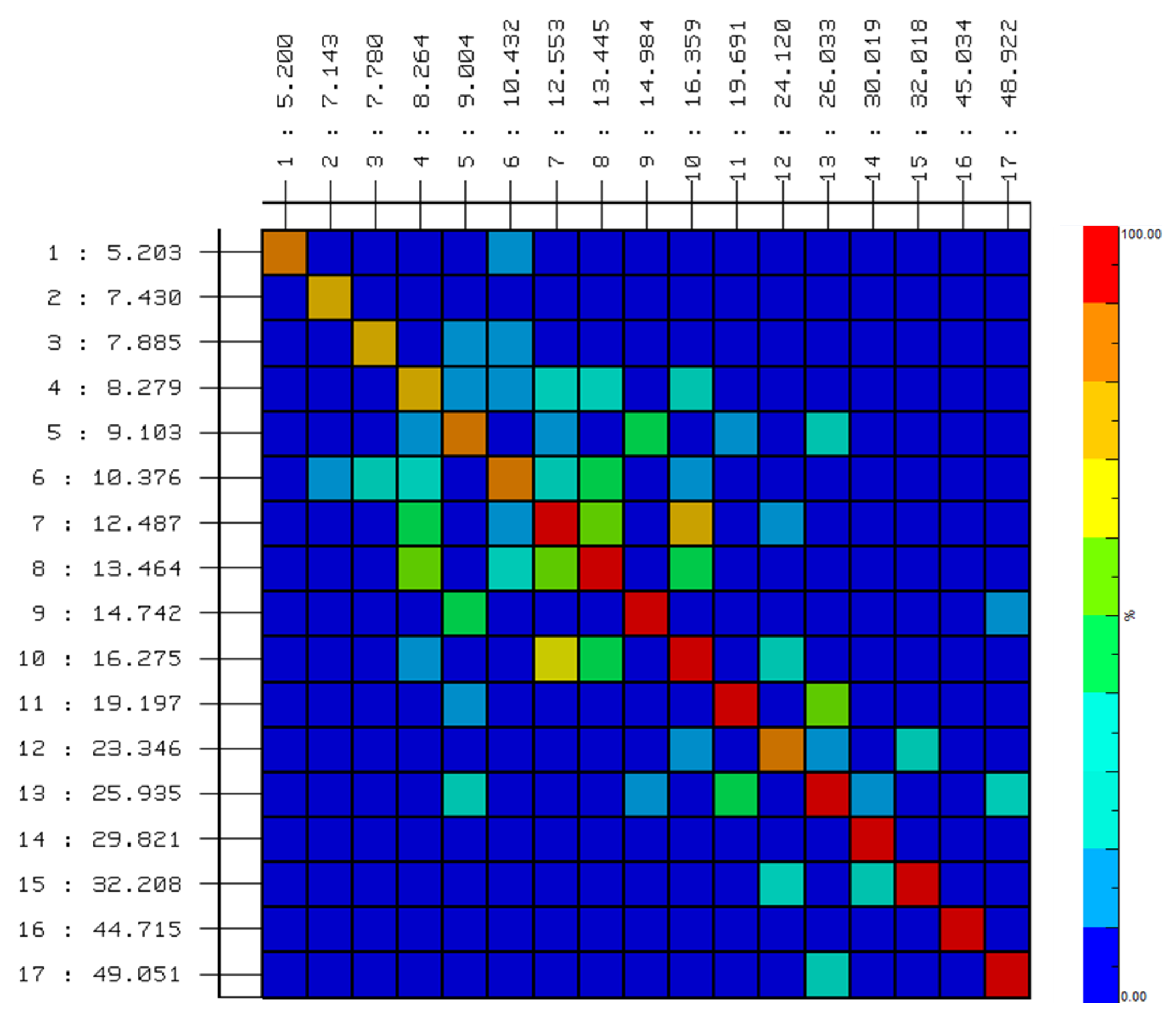
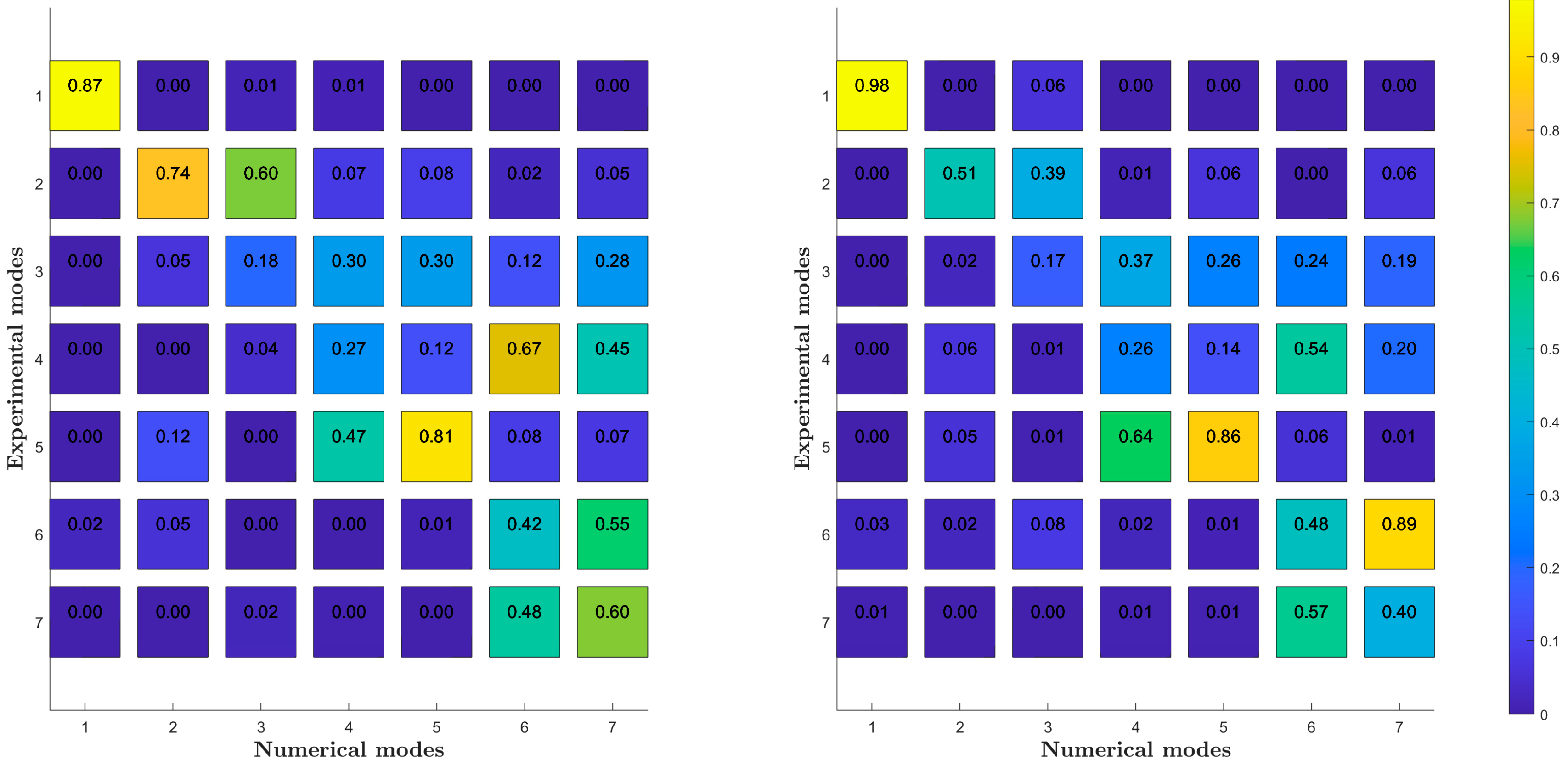
  • Looking at the Cross MAC matrix it is possible to see that the differences in the mode shapes are limited to the low frequencies mode shapes and mainly the wing torsional modes, due to the position of the moving masses positioned on the wing tip.
  • Based on the GVT data, it appears that the presence of a light non-symmetry in the real model makes it difficult to measure separate global symmetric and anti-symmetric torsional modes. They appear as two different modes at about the same frequency, involving each wing half separately. This generated a poor correlation in the Cross-MAC matrices, as reported in Figure 6b,c.
This unusual behavior is the main source of difficulty in producing a final well-correlated model. However, it has been decided not to try to completely recover the symmetry of the model, nor to try emulating the same behavior in the numerical model, but rather to leave a non-perfectly matched torsional behavior to test the robustness of the active control laws for flutter suppression.
After the GVT, a preliminary wind tunnel test session was scheduled, which aimed at the identification of the flutter behavior, before proceeding with the detailed modal updating phase that is based on both GVT and experimental flutter results.

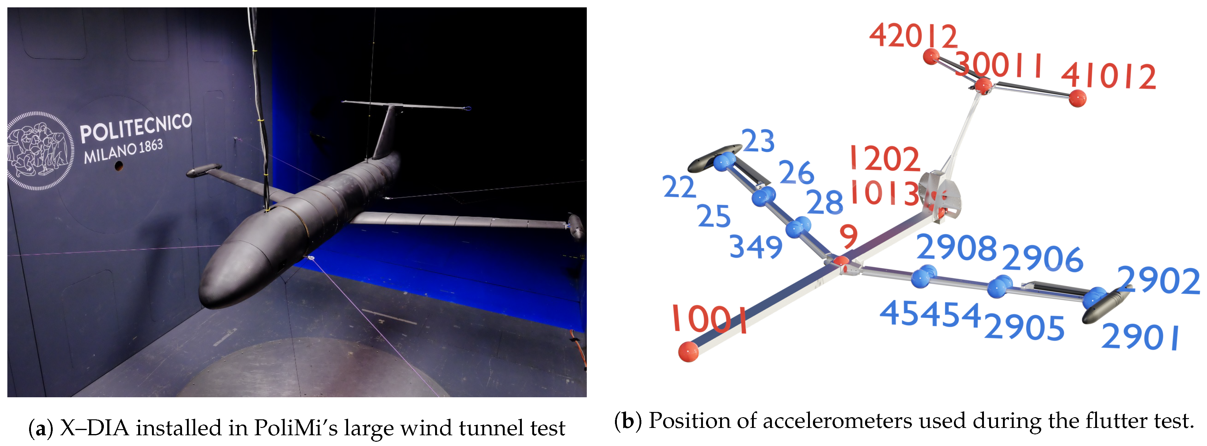
4. Preliminary Experimental Flutter Test

The wind tunnel flutter test campaign has been carried out in the PoliMi’s large Wind Tunnel, suspending the X–Dia model in a free–free configuration by means of elastic cables. The scope of this test campaign is to identify the flutter boundary keeping the overall aeroelastic trend under control, while the velocity increases.
The sensor layout is shown in Figure 7b and includes 20 embedded MEMS monoaxial accelerometers in addition to one capacitive triaxial accelerometer located in the CG of the complete model. The test session was remotely managed from the wind tunnel control room by an internet cable connected to the on-board system and laid along the front suspension cable. Additionally, two cables for the computer and the servo-actuators power supply were used. Figure 7a shows the X–Dia model installed inside the wind tunnel chamber.
For the assigned wind-tunnel velocities reported in Table 3, both anti-flutter mass configurations have been considered, and the complete model has been self-excited by different kinds of input excitation produced by oscillating the ailerons: sine sweep, impulse, band-limited white noise, and square wave. The constant band-limited white noise allowed us to perform a preliminary real-time flutter identification to demonstrate that the model is flutter-free until the maximum planned velocity when the anti-flutter device is turned on.
The next wind tunnel test session was aimed at the fully experimental flutter identification, considering when the anti-flutter device was turned off. Two different methodologies were adopted. The first one is based on the use of PolyMAX method, implemented in the LMS Test-lab [20,25], which is the same approach adopted during the GVT. The results, in terms of frequency and damping values, were also computed using an in-house code, based on the ARX approach [26].
Once the maximum speed was reached, the aeroelastic system appeared to be close to a zero-damping condition, so the velocity incremental step was reduced to 0.5 m/s. The wind tunnel test continued looking for the flutter point that was achieved at 41.5 m/s.

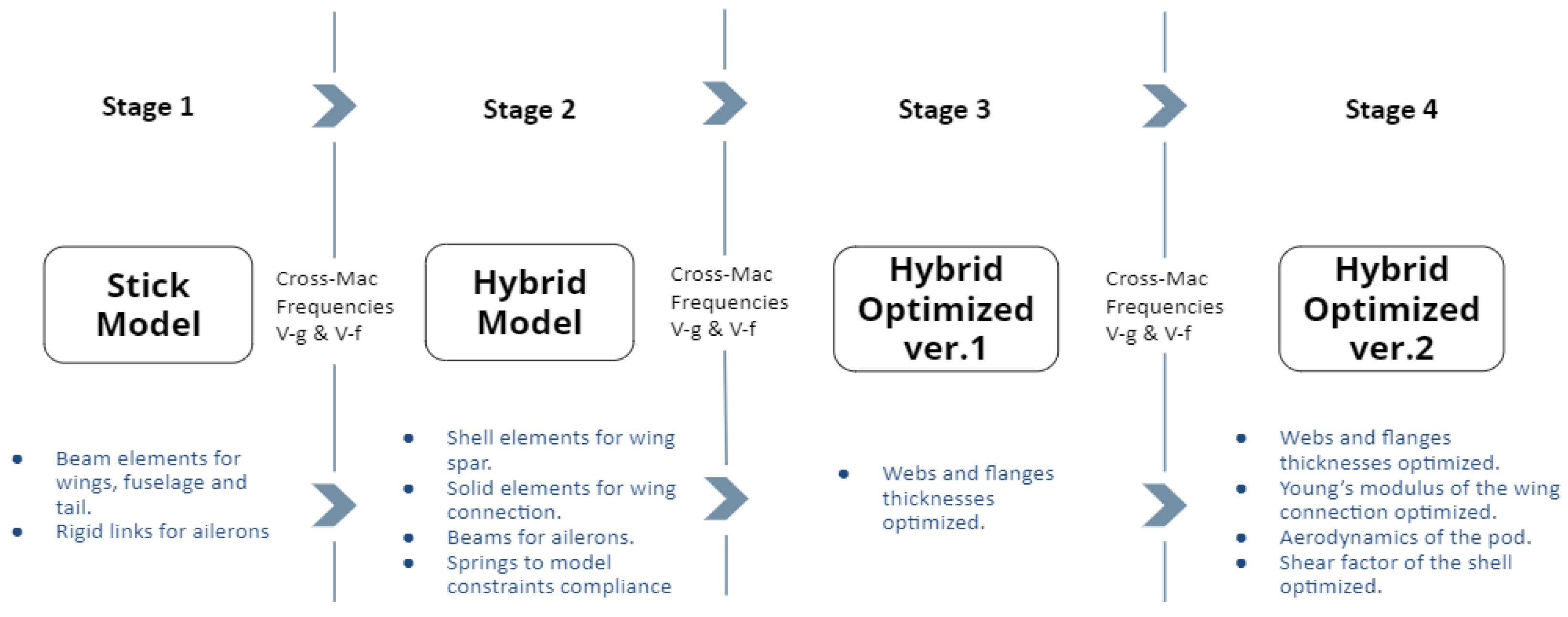
5. Structural Models

The need to have numerical models that correctly reproduce the features of interest can be traced back to the possibility of simulating the real structure, predicting the results of the analyses, as well as developing, designing, and tuning its response. Even if a large and complete set of tools is available, creating a well correlated mathematical model is not a linear and straightforward process but an iterative operation and the result of a compromise. This is especially true for wind tunnel aeroelastic models that are typically realized by single beams to which many and different elements are connected, such as the aerodynamic sectors, the local stiff elements like ribs to support the electric motors driving the control surfaces, local masses represented by sensors, as well as the cables. The goal of the correlations is based on a comparison among measured and predicted quantities, able to fully capture the aeroelastic behavior, such as the modal frequencies and mode shapes, as well the classical V g plots, while the natural choice to numerically model this kind of aeroelastic wind tunnel models, especially where the load carrying member is a beam, by classical stick model, sometimes it happens that they are not able to fully capture the actual aeroelastic behavior. This is what happened in the case of the X–Dia model that was forced to adopt a hybrid model in place of a simple stick model.
Some hypotheses have been introduced in the construction of the model to simplify the subsequent analyses without excessively compromising the final results. At the beginning, a classical stick model based on beam elements (Timoshenko formulation, including warping DoF, for the wing spar modeling; Euler–Bernoulli for the fuselage), concentrated masses, rigid elements, and aerodynamic behavior of a lifting surface, described with the Doublet Lattice Method (DLM), has been built. These hypotheses are justified in the perspective of achieving a correlated model. The efforts have been headed to catch a sufficient detail level to allow the FEM model to describe the global trend. The properties of beam elements have been extracted from analytical section calculations, combined with experimental and CAD measures. In addition, only certain structural modes are involved in the flutter mechanism and for this reason, they are ones that are worth focusing on during the correlation and the updating process.
During the correlation phase, involving frequencies, mode shapes, and V g plots comparisons, it appeared that the need to increase the fidelity of the model to capture the effect of local structural variations cannot be captured by the simple stick model, as will be further described in Section 7. Therefore, a new model, called hybrid, was implemented.
One of the difficulties in modeling the actual aeroelastic behavior by means of a simple stick model is due to the use of an open, omega section for the wing spar. Both the poor torsional stiffness typical of the open sections and the location of elastic axis outside the wing plane, due to the omega-shape, generating a strong coupling between the in-plane motion and the torsional one, confer to the X-DIA wing dynamic a significant complexity. Despite the possibility in MSC/NASTRAN to use beam elements controlling the position of the elastic center of the spar section, an adequate tuning phase has been requested to identify the correct value for the shear stiffness factor so as to correctly model the bending-torsion coupling.
Furthermore, structural elements with marked 3D characteristics, such as the connection between the wing and the fuselage, have shown a dynamics that may not be grasped with the stick model. The previous considerations, based on the preliminary experimental correlation phase, have highlighted the need to modify the initial stick model by modeling the wing spar by plate elements and the wing–fuselage connection by solid elements. The result is a hybrid model, as represented in Figure 8, with different level of detail depending on the actual impact of these zones on the overall dynamic behavior.
Another local modification has been necessary to correctly model the details of the connection between the wing and the anti-flutter pods. It consists of a concentrated mass linked with fairly flexible connections to a rigid section. The difference in stiffness of the components, together with its large distance from the axis of the aircraft, makes the impact of this model on the modal properties significant. To manage this issue, a dedicated elastic element has been introduced to model the connection between the wing tip and the attachment of the pod. Tuning the stiffness value of the spring allows to take into account possible compliance effects.
It has to be noted that, despite all the modifications made to the model refer to structural properties, the resulting effect is also to improve the aeroelastic correlation, due to their impact on the mode shapes and as consequence on the unsteady aerodynamic forces. Interesting and beneficial studies could embrace the aerodynamic formulation of the anti-flutter device, modeled using MSC/NASTRAN slender body formulation, but it does not fall within the goals of this work [27].

6. Model Updating Strategy

The wide and complete database, represented by the GVT results as well as by the preliminary wind tunnel flutter tests, described in Section 3 and Section 4, is the basis for the correlation process and later the updating phase. It must be taken into account that, especially for complex aeroelastic wind tunnel models, there are many components or unknown parameter values that prevent the best correlation level from being obtained. Unmodeled dynamics could be the cause for not reaching an acceptable correlation level. A typical solution to cover these discrepancies is fitting the experimental data changing model parameters in a least-square sense. This is at the core of the updating method herein employed. The modeling errors causing low correlation can be filled by the implementation of an optimization problem aiming at finding the model parameters values to minimize the numerical vs. experimental errors [28,29,30].
The so-called model updating is not straightforward and in most cases requires significant user experience. Various successful model updating methods have been developed to work on the matrices representing the dynamics of the system [29,31]. In the case of the X–DIA model, the updating problem has been formulated like a classical structural optimization process and solved thanks to the design sensitivity and optimization capabilities of SOL200 of MSC/NASTRAN [17]. This choice is mainly due to the possibility to use the same code and the same FEM models for both the updating process and the aeroelastic assessment.

6.1. Optimization Problem Setup

The optimization problem setting is based on some hypotheses:
  • Many optimizers give the possibility to base the error to minimize many kinds of response variables and flutter velocity as well. Even if the scope of these activities is to capture the aeroelastic behavior with special attention on the flutter point, a purely structural-based formulation has been preferred. A restricted number of variables coming into play can guarantee a better convergence and stronger robustness of the results. The aeroelastic effects have been recovered in a second phase. Thus, the objective function is defined to minimize the differences in the natural frequencies and the differences in the mode shapes between the numerical model and the GVT results.
  • The model configuration subjected to optimization has been limited only to the anti-flutter mass in backward position, which is the one prone to flutter. It would have been possible to carry out a double optimization on both configurations, but the actual difference between the two is due to the position of a single mass. In this way, the second mass configuration could be used as a check for the correctness of the optimal solution.
The optimization problem requires us to define an error function to be minimized and consists of the differences between numerical model outputs and the desired values, namely the experimental data. The function passed to the optimizer, thanks to DEQATN and DRESP2 MSC/NASTRAN cards [17], has the form:
J f 1 , f 2 , f 3 = f G V T 1 f 1 f G V T 1 2 + f G V T 2 f 2 f G V T 2 2 + f G V T 3 f 3 f G V T 3 2
No weight-sum squared function has been used, since the actual cost function contains the dimensionless relative errors between f GVT i , the measured natural frequencies, and f i , the numerical frequencies, and it has been assumed that they all have the same impact on the flutter mechanism and the same accuracy. Equation (1) is composed of the first three structural modes frequencies since they are the ones taking part in the aeroelastic instability. Indeed, the X–DIA presents a typical coupled bending–torsional flutter instability: the 1st is a bending mode, the 2nd and 3rd are two coincident torsional modes, anti-symmetric and symmetric, respectively.
One of the key aspects during model updating is represented by the choice of the design variables, i.e., the properties of the structure that are subject to modifications during the process. They have to be representative of the uncertainties resulting from the modeling process, but at the same time, they have to guarantee an updated model representative of the physical one, while few design variables allow to recover systematic error in global stiffness and mass representation, a higher number of design variables allows us to correct local modeling errors.
The design variables considered here are the thickness of the plates of the wing spar, chosen for the possibility to recover all the unmodeled details that in some way can impact on the stiffness distribution. However, to avoid unreasonable thickness changes, it is necessary to impose some user-defined constraint. The mass of the model is experimentally known and fixed, so accordingly to the thickness the density must also vary in such a way that the total mass does not change. The DLINK card of MSC/NASTRAN has provided an optimization constraint to specify the density as a function of independent variables according to an adaptation law stated by (Equation (2)):
ρ ( t 1 , t 2 , t 3 ) = c 1 t 1 + c 2 t 2 + c 3 t 3
where t 1 , t 2 , and t 3 are thicknesses of spar parts (central and vertical webs and side flanges, see Figure 9) and c 1 , c 2 , and c 3 are constant coefficients, introduced by means of DTABLE MSC/NASTRAN card, linking the changes in thicknesses to the total mass of the structure, in order to have it constant. Each part of the spar can have an independent change (fixed spanwise), but the updated value of the density has to consider all of these, each with a different weight based on their portion of the overall volume.
c i = V n o m i V t o t t n o m i ρ n o m
where:
  • V n o m 1 
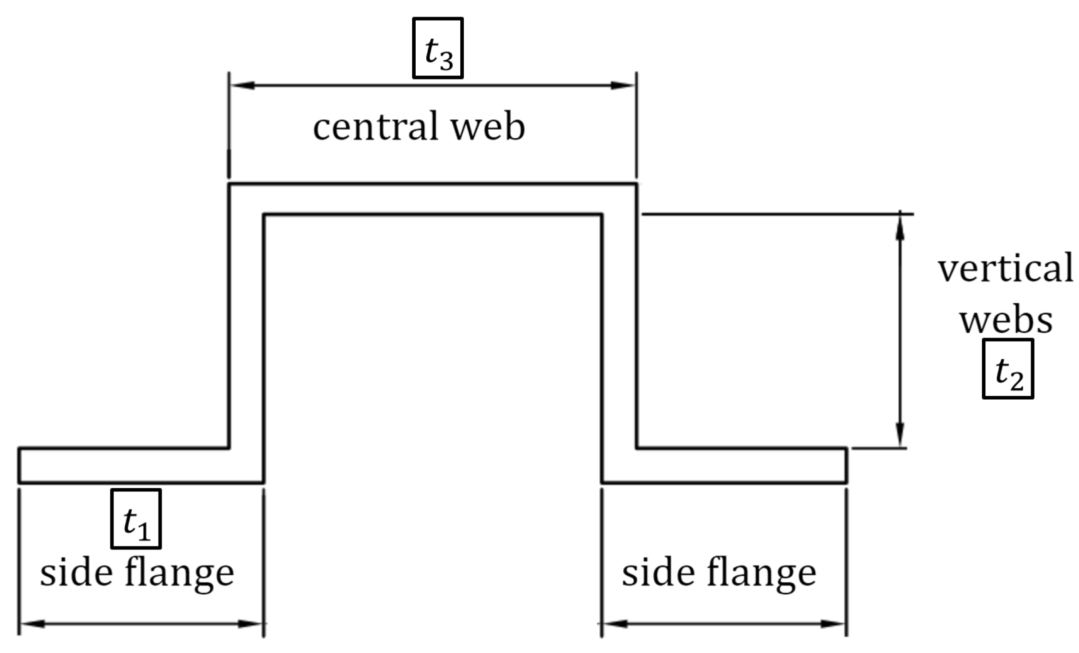
is the volume relating to part 1 of the omega-shaped spar with nominal values;
  • V t o t = V n o m 1 + V n o m 2 + V n o m 3 is the total volume in the nominal configuration;
  • t n o m 1 is the nominal thickness relating to part 1 of the omega-shaped spar;
  • ρ n o m is the density in nominal configuration of the spar material.
The scope of this optimization setting is to grasp the correct inertia allocation of the wing spar. The density constraint has been included to fix the total value of the mass and allow the algorithm to distribute the inertia independently (mass properties are shown in Table 4).
The differences in the mode shapes between the numerical model and the GVT data could be minimized and included in the optimization loop as well, using for example the related MAC values. The cost function weighted MAC term has the form of Equation (3).
J M A C = W s h a p e i ( 1 M A C r e d )
where the M A C r e d is an entry of the MAC red matrix corresponding to a reduced set of key nodes W s h a p e i is the weight matrix containing possibly different weights for the entries of the MAC red .
Despite modal shapes having a great impact upon the flutter mechanism, this last term has not been included in the overall cost function but just used as a check after every optimization loop to track the mode shapes correlation obtained. Indeed, including the mode shapes into the objective function significantly increases the computational cost of the optimization process due to the need to face the non-linearities introduced.

6.2. Updating Phase

As already mentioned, the goal is to correctly capture the flutter behavior, but the optimization carried out involves only modal parameters (Section 6.1), i.e., modes at zero speed. When the aerodynamic forces come into play, the matrices of the system change according to the Mach number and the reduced frequency. To also include the flutter contribution within the procedure, the optimization runs have been performed while constantly monitoring the aeroelastic response. Optimization runs have been alternated with flutter analyses to check the current state and to tune the process in order to fit the experimental data. This allowed us to gradually study the flutter prediction compared to the experimental one. Thus, the union of these two techniques leads to a complete updating analysis of the aeroelastic behavior of the wind tunnel model.
The results of an updating phase strictly depends on the choice of the design variables and their allowable variation. Thus, starting from the hybrid finite element model, different configurations of design variables have been explored.
In a first step, a limited number of design variables, i.e., the thickness of the horizontal and vertical walls of the omega, kept constant spanwise, was adopted. The algorithm converged in four iterations, with a reduction of the cost function of one order of magnitude from 4.37 × 10 2 to 6.48 × 10 3 . In a second step, a more aggressive optimization was applied: a larger number of design variables was introduced, which also impacted the stiffness of the wing–fuselage connection block, the shell’s transverse flexibility, and aerodynamic effect of the anti-flutter device. The algorithm required three iterations and reduced the cost function of another order of magnitude up to 2.06 × 10 4 . In particular, the algorithm showed that the shell transverse behavior is a key factor in representing the real model dynamics. Initially, the shell shear factor was listed as a design variable and was included in the optimization loop, but the algorithm tendency to increase it drastically suggested to the authors to not involve it in the optimization loop, but rather to consider infinite transverse rigidity shell elements as the starting point for the second optimization phase.
The model evolution is presented in Figure 10 with the variables trend in Table 5 and the obtained results are discussed in next Section 7.

7. Correlation and Updating Results

During the activities herein presented, four FEM models have been developed: a stick model (Section 5), a hybrid model (Section 5), and optimized models version 1 and version 2 (Section 6.2).
The correlation starts reporting the comparison of the low frequency modes in terms of frequencies and mode shapes. Table 6 compares the first seven GVT frequencies with the ones obtained using the stick and the hybrid models, respectively. It is possible to see that the hybrid model better captures the dynamic properties than the stick one, even if an updating phase is still necessary due to the large frequency error present.
Figure 11 shows the Cross MAC matrix comparing the mode correlation among the free-suspended GVT mode shapes and the free-suspended numerical ones based on the stick model and the hybrid model, respectively. The choice to build the MAC matrices with the free-suspended mode shapes can be traced back to their capability to mostly represent the wind tunnel model behavior since both experimental and numerical modal analyses have been conducted with the same model configuration for the aeroelastic tests.
Starting from this situation, the updating activities aim at the modification of the structural model to improve the correlation in the rear mass configuration since they are the most important factor from the flutter behavior point of view.

Modal Correlation

Starting from the stick model results, it can be seen that after the modifications are introduced into the model, the correlation with the bending modes is strongly improved, in particular with the first mode that is the one involved in flutter instability. The experimental–numerical correlation level has been measured and evaluated by means of model validation techniques (Section 3).

Natural Frequencies Correlation

Attention has been focused on the lower frequency modes because they are the most significant for the dynamic behavior of the structure, especially for the flutter phenomenon. The wind tunnel tests have shown that the main flutter instability involves the 1st and 3rd modes, respectively, out-of-plane symmetric bending and symmetric torsional of the wing. Table 7 compares the frequencies of the first three modes of the mass-backward configuration since they are the ones used for the optimization process. The flutter results have been checked using different sets of modes, reaching a total of 40 modes to compute the response and looking at the possible variations. The result remained unaffected.
Starting from the stick model results, a very limited error can be noted (wheb dealing with modal frequencies, a threshold error of 1–2% is usually considered). Nevertheless, its prediction for flutter behavior is very bad, as described below in this section, demonstrating that a good correlation level on modal frequencies is not sufficient to also have the same level for aeroelastic ones. The transition from the stick model to the hybrid one has not produced better results concerning the the frequency errors but has paved the way for a better description in terms of mode shapes. For this reason the updating process has been applied to the hybrid model, thus setting up an optimization problem aiming at the minimization of the frequency errors of the first three low frequency modes, i.e., the first bending and two torsional ones working mainly on the stiffness of the wing spar and the wing–fuselage connection.
During the first step, updating only three model parameters has updated, i.e., the three wing spar thicknesses describing the Omega section, keeping them fixed spanwise, so to correct the wing stiffness distribution in a global fashion. In the objective function the frequencies to be reached have been set equal to f G V T 1 = 5.2 Hz, f G V T 2 = 7.45 Hz, and f G V T 3 = 7.45 Hz.
As already anticipated, the reason why the frequencies f G V T 2 and f G V T 3 do not coincide with GVT’s results is due to the fact that the numerical model is perfectly symmetric showing two torsional modes (i.e., symmetric and anti-symmetric) with the same modal participation of left and right half wings. On the contrary, the actual physical model shows a slightly asymmetric behavior able to split any torsional mode into two separate modes with different participation on left and right side half wings (see Figure 12). This partially justifies the high error on the second torsional mode. In terms of the final design variables, the solution obtained shows a thickening of the vertical webs and side flanges of the spar, which intends to increase the torsional inertia and so the related frequencies, and a lightening of the central web that tries to decrease the bending frequency.
During the second step, a more extended model tuning was applied to improve the correlation level. The set of design variables were defined looking at the sensitivity of modal results showing that:
  • Decreasing the Young modulus of the wing root connection elements allows us to decrease the first bending frequency.
  • Decreasing the Young modulus or the thickness of the top flange of the spar mainly decreases the bending frequency.
  • Changing the webs and flanges thicknesses of the spar impact on the torsional frequencies.
At the same time, further modification to the finite element model was applied, such as:
  • Transverse shear flexibility set in order to have an infinitely rigid in transverse direction plate and trying to increase the torsional stiffness of the wing.
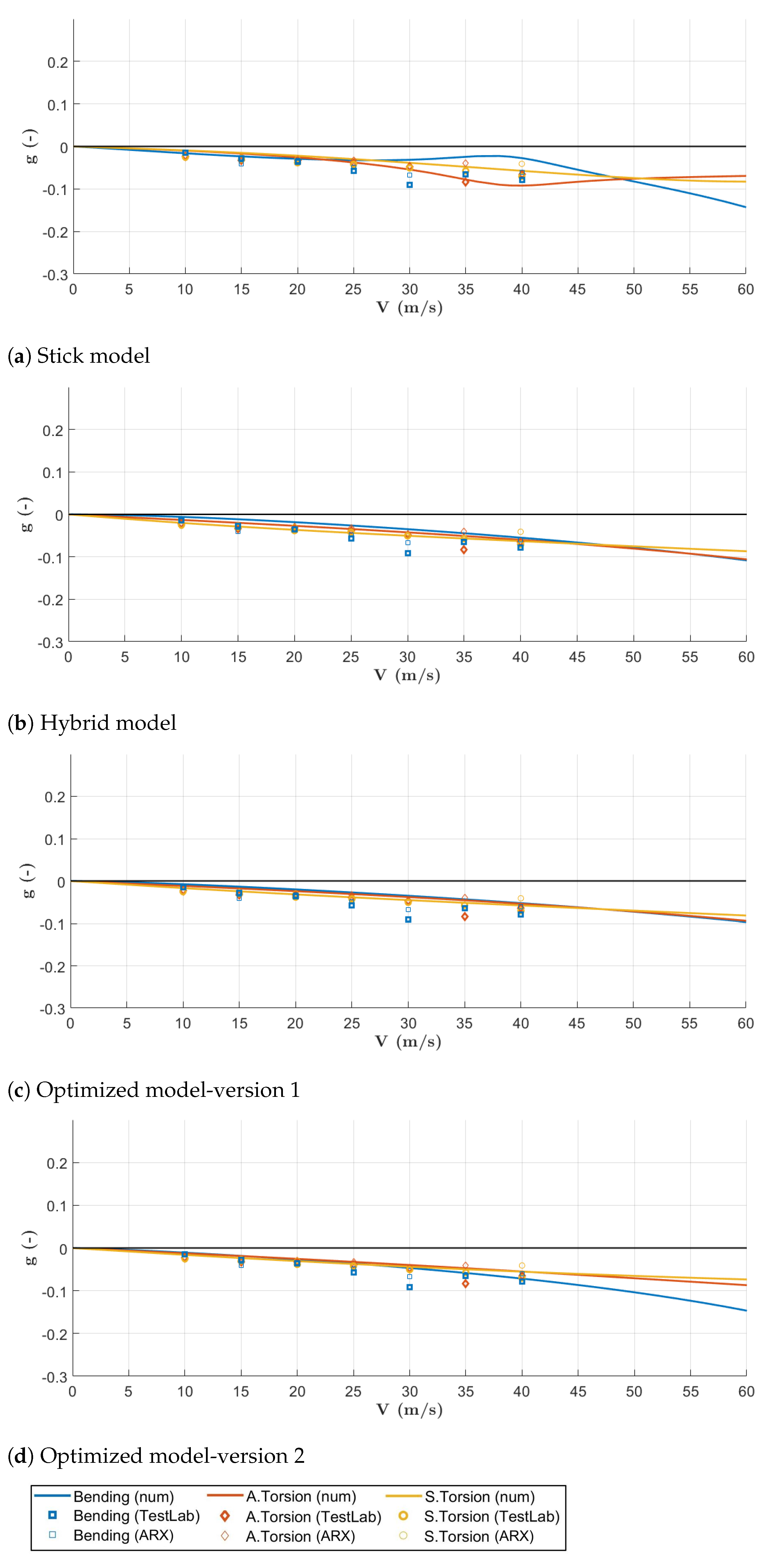
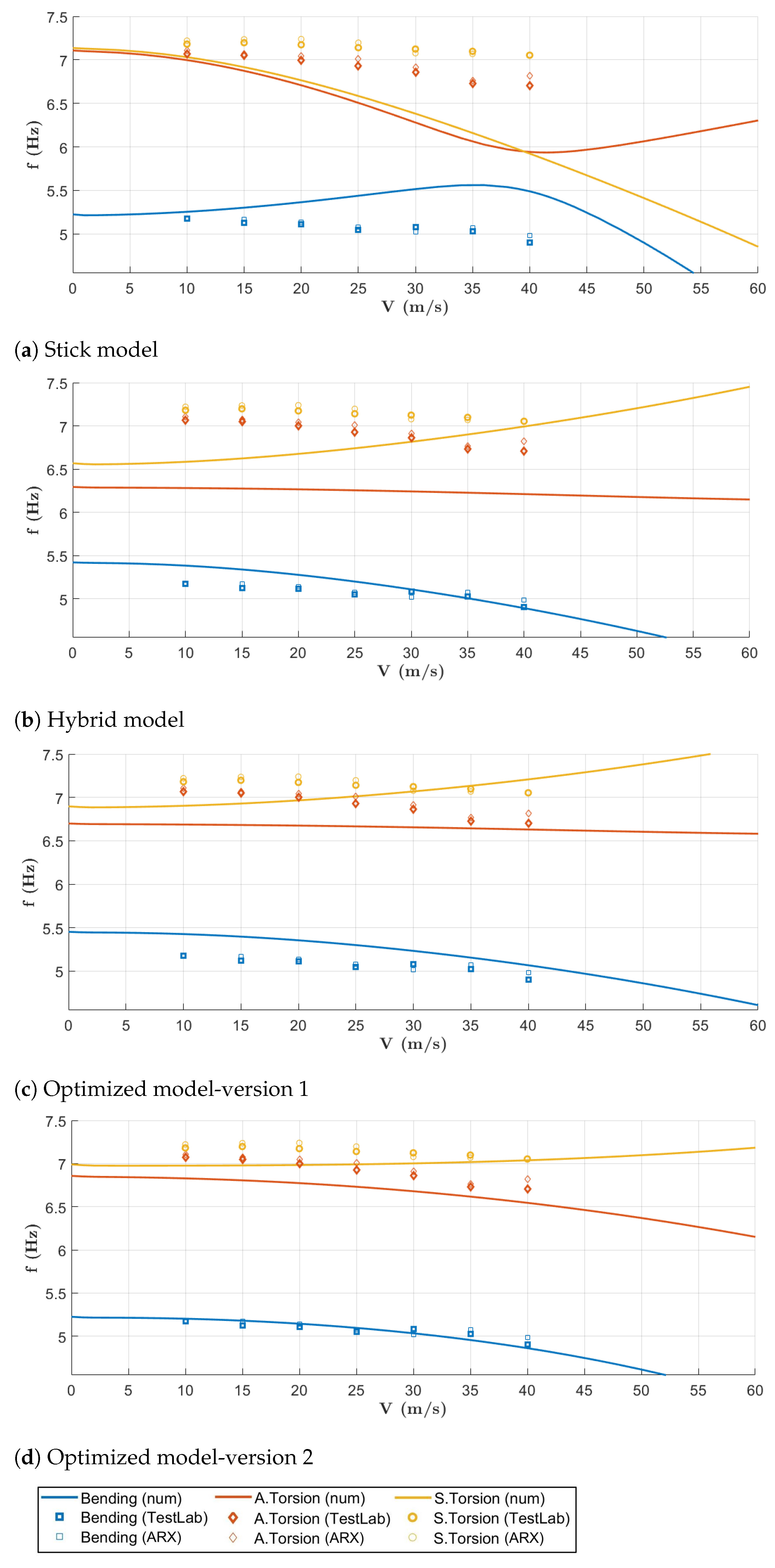
  • Classical and not burdensome slender body aerodynamics formulation of the pod was introduced during the flutter analysis, to better reproduce the flutter behavior of the updated model.
The second updating step allowed us to improve the correlation level that will be now discussed in detail. Looking at the modal frequencies reported in Table 7 and the Cross MAC matrices ([24]) of Figure 13, it is possible to draw the following remarks:
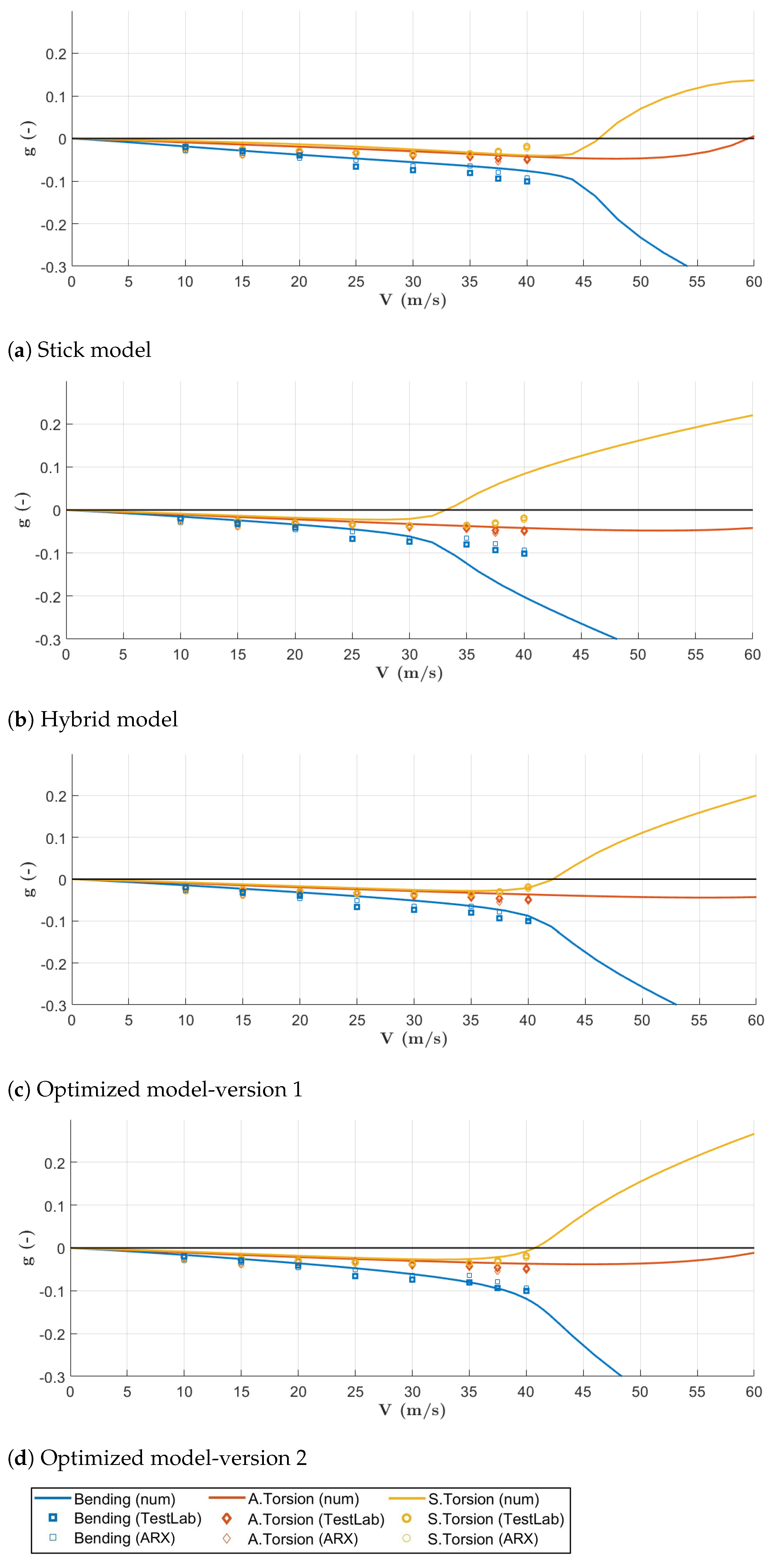
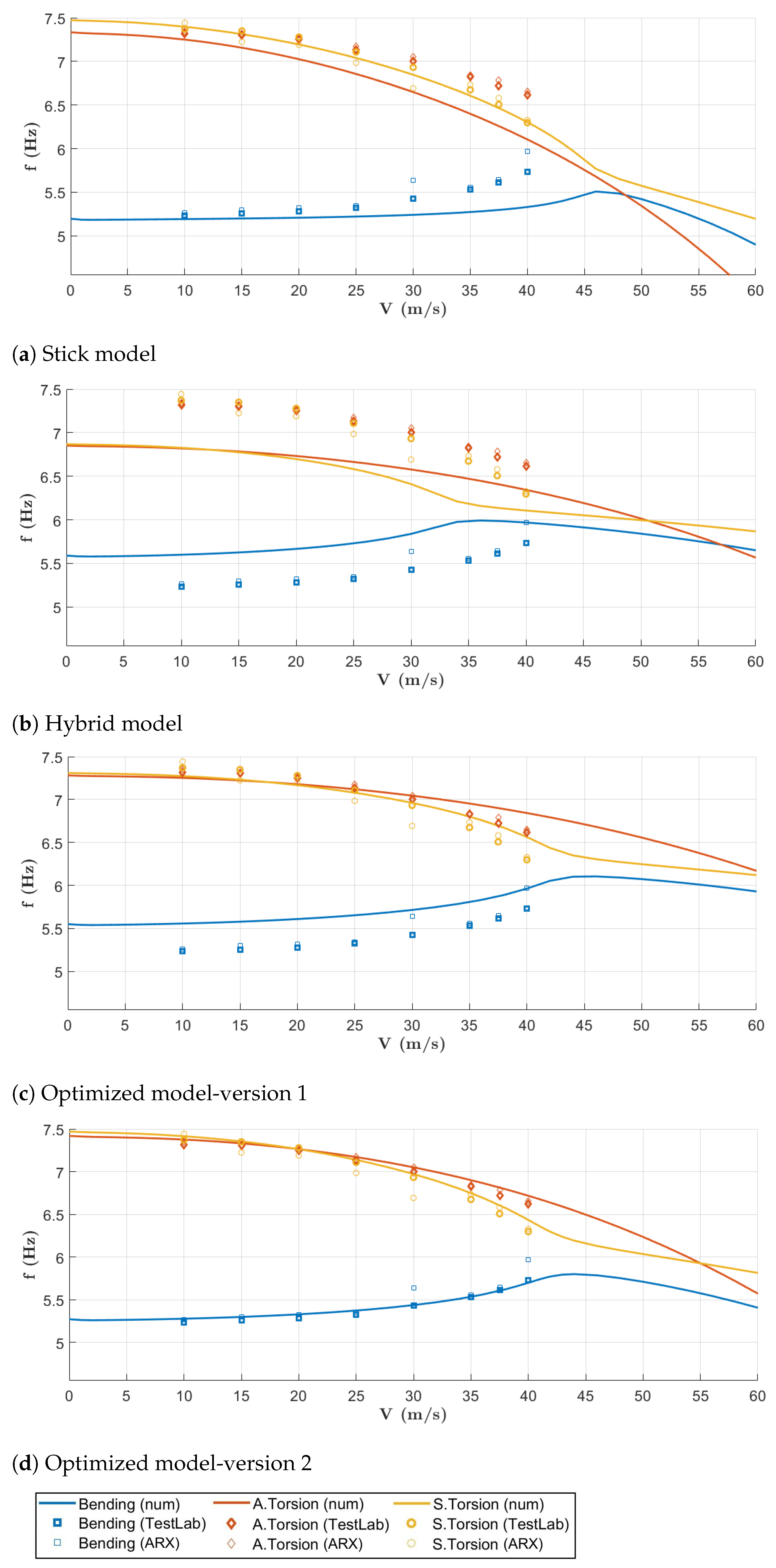
  • With the last optimization run, the error committed on the modal frequencies falls below an adequate threshold, thus achieving an excellent level.
  • Starting from Hybrid model, the updating process has managed to reduce the error at every step, as can be seen in Table 7. The algorithm has impacted the target frequencies of 0.72% for the 1st symmetric bending, 6.28% for the 1st anti-symmetric torsional, and 6.4% for the 1st symmetric torsional, during the first optimization loop; the values were 5.05%, 1.92%, and 2.19% during the second loop.
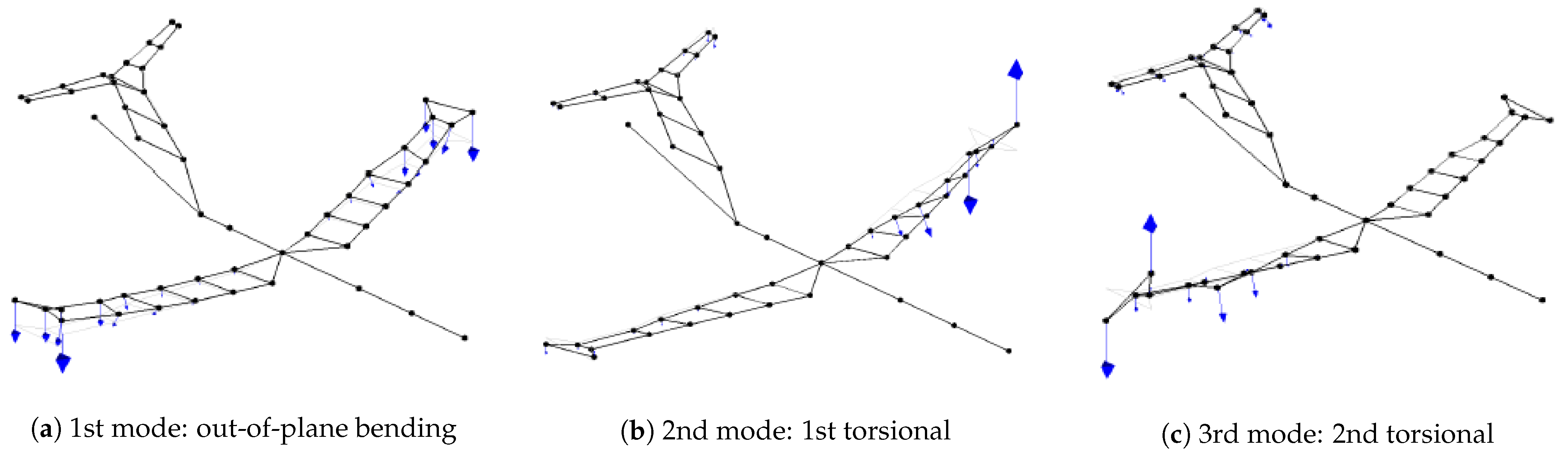
  • The 1st first bending mode has been captured very well, both in terms of frequency and shape. This is very important because the flutter mechanism involves the exactly 1st bending and the 2nd torsional (mode # 3).
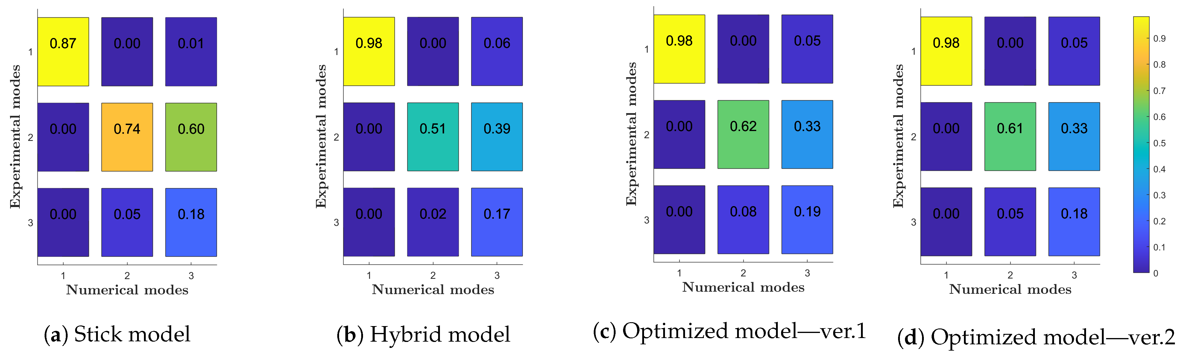
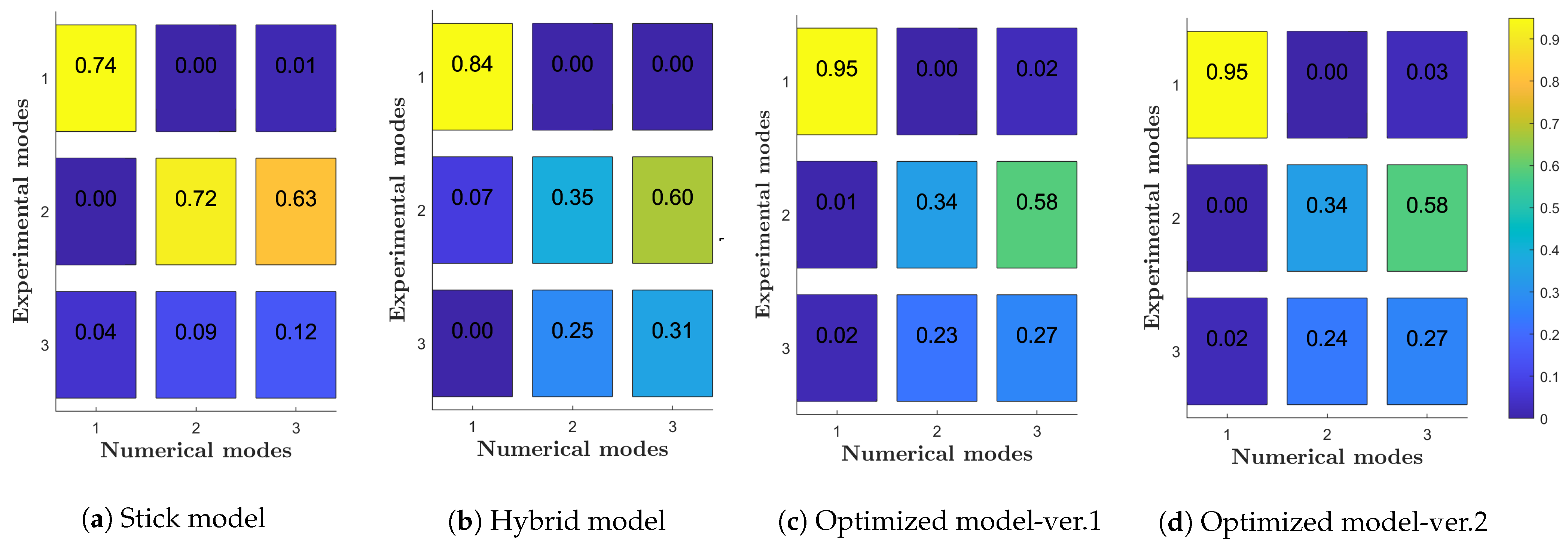
  • Due to the presence of two split torsional modes, as identified during the GVT campaign and reported Figure 12b,c, due to the fact that the actual wind tunnel model is not perfectly symmetric, the correlation results are still poor.
Despite this low correlation related to the torsion modes, the frequency error reduction as well the model improvement allowed us to capture the global aeroelastic behavior and it will be now discussed.
Concerning the flutter instability, commonly it is studied in terms of V g and V f plot typically obtained using the well known p-k method [32], where the aeroelastic damping g is the quantity tracked to identify flutter onset; the instability is associated with negative damping, reflected in a positive value of g.
In such a case, these values have been extracted through post-processing activities. No dedicated Operational Modal Analyses were carried out.
Figure 14 and Figure 15 depict the trend of the three modes involved in the flutter mechanism and compare the experimental results with the numerical ones. The preliminary wind tunnel tests had the scope to identify the flutter; no active flutter suppression controllers were available at that time. Thus, the experimental velocities were limited by the flutter point (Table 3). The error in predicting the flutter velocity is summarized in Table 8. During these tests, the presence of unsteady aerodynamic forces practically made the left/right torsion difference no more significant and almost disappeared during the identification.
Looking at Table 7 and Table 8 it is possible to say that both step 1 and step 2 updated models have produced significant results in terms of error reduction with respect to the experimental flutter test results. In the first instance, the hybrid model alone did not improve the error in flutter velocity prediction but did prepare the ground for the optimization process. In fact, after the second updating loop, the final model was the best compromise between the errors in the flutter velocity and frequency prediction and the aeroelastic behavior represented in the V g plot.
Of special interest to us is the correlation obtained after the updating process in the case of the model with the mass of the safety flutter device in the forward position, which has not been directly involved in the updating. Indeed, since in reality the only difference between the two configurations is represented by the position of two concentrated masses on the tips, it is reasonable to expect some progress in the correlation level, demonstrating the global meaning of the model changes made.
Concerning the modal parameters, the modes participating in flutter refined from time to time their correlation, in particular the 1st bending mode (Table 9 and Figure 16). For the two torsional modes, the improvements were limited by the non-symmetry of the real model, as explained previously.
Looking at the flutter behavior reported in Figure 17 and Figure 18, the V g and V f plots have confirmed what was expected: the updating process applied to the FEM model with the safety mass in the backward positions produced an updated model able to capture the global aeroelastic behavior also in the case of the safety masses in the forward position.

8. Conclusions

This paper summarized the activity carried out to finalize the aeroelastic model of the X–DIA wind tunnel model. It proposed an overview for model updating and its role in aircraft development.
The first part of the work focused on FEM model developments. Starting from a typical stick model usually adopted for aeroelastic models, the model was improved into a hybrid model based on a plate model of the main spar that is more suitable to capture the structural behavior of the wing. This choice was mainly due to the particular omega shape of the wing cross-section that naturally couples the in-plane bending to the torsion modes. Then, solid elements were adopted to model the blocks connecting the wing spar to the fuselage. Special attention was devoted to the modeling of the anti-flutter pods due to their strong impact on the wing dynamic response.
After the correlation process with the GVT results, the updating process was started, conceived, and implemented as a typical structural optimization problem. Two different updating loops were performed, with different numbers of design variables. The correlation and updating process was complicated by the slight non symmetry of the physical model, making it impossible to reach a perfect correlation among the numerical and experimental torsion modes. Despite these difficulties, the updating process was successfully completed, thus obtaining a numerical dynamic model able to perfectly reproduce the global aeroelastic behavior measured during the wind tunnel testing, with a final error on the flutter velocity around 1.2%. The updated dynamic model will be used as the starting point to generate the state-space aeroelastic model to be used for the development of dedicated flutter suppression control strategies.

Author Contributions

Data curation, F.L.B.; Funding acquisition, S.R.; Investigation, D.D.L., F.L.B., and A.D.G.; Methodology, A.D.G.; Software, D.D.L. and F.L.B.; Supervision, A.D.G. and S.R.; Validation, D.D.L.; Visualization, D.D.L. and F.L.B.; Writing—original draft, D.D.L., F.L.B., A.D.G. and S.R. All authors have read and agreed to the published version of the manuscript.

Funding

This research received no external funding.

Institutional Review Board Statement

Not applicable.

Informed Consent Statement

Not applicable.

Acknowledgments

Support by the Federal Aviation Administration as well as contributions by Wael Nour and Sohrob Mottaghi from the FAA are gratefully appreciated. A special thanks goes to Eli Livne of University of Washington.

Conflicts of Interest

The authors declare no conflict of interest.

Abbreviations

CGCenter of Gravity
DOFDegree of Freedom
DLMDoublet-Lattice Method
FEMFinite Element Method
FRFFrequency Response Function
MACModal Assurance Criterion
X-DIAeXperimental Dipartimento di Ingegneria Aerospaziale

References

  1. Bisplinghoff, R.; Ashley, H.; Halfman, R. Aeroelasticity; Dover Publications, Inc.: Mineola, NY, USA, 1955; Chapters 12–13. [Google Scholar]
  2. Miller, S.; Vio, G.A.; Cooper, J.E.; Vale, J.; da Luz, L.; Gomes, A.; Lau, F.; Suleman, A.; Cavagna, L.; De Gaspari, A.; et al. SMorph—Smart Aircraft Morphing Technologies Project. In Proceedings of the 51th AIAA/ASME/ASCE/AHS/ASC Structures, Structural Dynamics and Materials (SDM) Conference, Orlando, FL, USA, 12–15 April 2010. [Google Scholar] [CrossRef]
  3. Pankonien, A.M.; Durscher, R.; Bhagat, N. Parametric 3D-Printable Flutter Model for Constrained Aeroelastic Scaling. In Proceedings of the AIAA Scitech 2019 Forum, San Diego, CA, USA, 7–11 January 2019. [Google Scholar]
  4. Livne, E. Aircraft active flutter suppression: State of the art and technology maturation needs. J. Aircr. 2018, 55, 410–452. [Google Scholar] [CrossRef]
  5. Bond, V.L.; Canfield, R.A.; Suleman, A.; Blair, M. Aeroelastic Scaling of a Joined Wing for Nonlinear Geometric Stiffness. AIAA J. 2012, 50, 513–522. [Google Scholar] [CrossRef]
  6. Pereira, P.; Almeida, L.; Suleman, A.; Bond, V.; Canfield, R.; Blair, M. Aeroelastic Scaling and Optimization of a Joined-Wing Aircraft Concept. In Proceedings of the 48th AIAA/ASME/ASCE/AHS/ASC Structures, Structural Dynamics, and Materials Conference, Honolulu, HI, USA, 23–26 April 2007. [Google Scholar] [CrossRef]
  7. Moreno, C.P.; Gupta, A.; Pfifer, H.; Taylor, B.; Balas, G.J. Structural model identification of a small flexible aircraft. In Proceedings of the 2014 American Control Conference, Portland, OR, USA, 4–6 June 2014; pp. 4379–4384. [Google Scholar] [CrossRef]
  8. Meddaikar, Y.M.; Dillinger, J.; Klimmek, T.; Krueger, W.; Wüstenhagen, M.; Kier, T.M.; Hermanutz, A.; Hornung, M.; Rozov, V.; Breitsamter, C.; et al. Aircraft Aeroservoelastic Modelling of the FLEXOP Unmanned Flying Demonstrator. In Proceedings of the AIAA Scitech 2019 Forum, San Diego, CA, USA, 7–11 January 2019; American Institute of Aeronautics and Astronautics: San Diego, CA, USA, 2019. [Google Scholar] [CrossRef] [Green Version]
  9. Takarics, B.; Patartics, B.; Luspay, T.; Vanek, B.; Roessler, C.; Bartaševičius, J.; Koeberle, S.J.; Hornung, M.; Teubl, D.; Pusch, M.; et al. Active Flutter Mitigation Testing on the FLEXOP Demonstrator Aircraft. In Proceedings of the AIAA Scitech 2020 Forum, Orlando, FL, USA, 6–10 January 2020; American Institute of Aeronautics and Astronautics: Orlando, FL, USA, 2020. [Google Scholar] [CrossRef] [Green Version]
  10. Wüstenhagen, M.; Süelözgen, O.; Ackermann, L.; Bartaševičius, J. Validation and Update of an Aeroservoelastic Model based on Flight Test Data. In Proceedings of the 2021 IEEE Aerospace Conference, Big Sky, MT, USA, 6–13 March 2021; pp. 1–18. [Google Scholar] [CrossRef]
  11. Zhao, W.; Gupta, A.; Miglani, J.; Regan, C.D.; Kapania, R.K.; Seiler, P.J. Finite Element Model Updating of Composite Flying-wing Aircraft using Global/Local Optimization. In Proceedings of the AIAA Scitech 2019 Forum, San Diego, CA, USA, 7–11 January 2019; American Institute of Aeronautics and Astronautics: San Diego, CA, USA, 2019. [Google Scholar] [CrossRef]
  12. Ricci, S.; Scotti, A.; Cecrdle, J.; Malecek, J. Active control of three-surface aeroelastic model. J. Aircr. 2008, 45, 1002–1013. [Google Scholar] [CrossRef]
  13. De Gaspari, A.; Ricci, S.; Riccobene, L.; Scotti, A. Active aeroelastic control over a multisurface wing: Modeling and wind-tunnel testing. AIAA J. 2009, 47, 1995–2010. [Google Scholar] [CrossRef]
  14. Ghiringhelli, G.; Lanz, M.; Mantegazza, P. A comparison of methods used for the identification of flutter from experimental data. J. Sound Vib. 1987, 119, 39–51. [Google Scholar] [CrossRef]
  15. Marchetti, L.; De Gaspari, A.; Riccobene, L.; Toffol, F.; Fonte, F.; Ricci, S.; Mantegazza, P.; Livne, E.; Hinson, K.A. Active Flutter Suppression Analysis and Wind Tunnel Studies of a Commercial Transport Configuration. In Proceedings of the AIAA Scitech 2020 Forum, Orlando, FL, USA, 6–10 January 2020; p. 1677. [Google Scholar] [CrossRef]
  16. French, M.; Kolonay, R.M. Demonstration of structural optimization applied to wind-tunnel model design. J. Aircr. 1992, 29, 966–968. [Google Scholar] [CrossRef]
  17. MSC. Nastran Design Sensitivity and Optimization User’s Guide; MSC/Software Corporation: Santa Ana, CA, USA, 2005. [Google Scholar]
  18. DeGaspari, A.; Mannarino, A.; Mantegazza, P. A Dual Loop Strategy For The Design of a Control Surface Actuation System with Nonlinear Limitations. Mech. Syst. Signal Process. 2017, 90, 334–349. [Google Scholar] [CrossRef]
  19. Inman, D.J.; Singh, R.C. Engineering Vibration; Prentice Hall: Englewood Cliffs, NJ, USA, 1994; Volume 3. [Google Scholar]
  20. Peeters, B.; Guillaume, P.; Van der Auweraer, H.; Cauberghe, B.; Verboven, P.; Leuridan, J. Automotive and aerospace applications of the PolyMAX modal parameter estimation method. Proc. IMAC 2004, 22, 1. [Google Scholar]
  21. Schwarz, B.J.; Richardson, M.H. Experimental modal analysis. CSI Reliab. Week 1999, 35, 1–12. [Google Scholar]
  22. Rockling, G.Y. A comparison of H1, H2 and HV frequency response functions. In Proceedings of the 3rd International Modal Analysis Conference, Orlando, FL, USA, 28–31 January 1985; pp. 272–278. [Google Scholar]
  23. Larson, C.; Zimmerman, D.; Marek, E. A comparative study of metrics for modal pre-test sensor and actuator selection using the JPL/MPI testbed truss. In Proceedings of the Dynamics Specialists Conference, Hilton Head, SC, USA, 21–22 April 1994; p. 1689. [Google Scholar]
  24. Ewins, D. Model validation: Correlation for updating. Sadhana 2000, 25, 221–234. [Google Scholar] [CrossRef]
  25. Peeters, B.; Van der Auweraer, H.; Guillaume, P.; Leuridan, J. The PolyMAX frequency-domain method: A new standard for modal parameter estimation? Shock Vib. 2004, 11, 395–409. [Google Scholar] [CrossRef]
  26. Diversi, R.; Guidorzi, R.; Soverini, U. Identification of ARX and ARARX models in the presence of input and output noises. Eur. J. Control. 2010, 16, 242–255. [Google Scholar] [CrossRef]
  27. MSC. Nastran Aeroelastic Analysis User’s Guide; MSC/Software Corporation: Santa Ana, CA, USA, 2005. [Google Scholar]
  28. Prananta, B.; Kanakis, T.; Vankan, J.; van Houten, R. Model updating of finite element model using optimisation routine. Aircr. Eng. Aerosp. Technol. 2016, 88, 665–675. [Google Scholar] [CrossRef]
  29. Mottershead, J.; Friswell, M. Model Updating In Structural Dynamics: A Survey. J. Sound Vib. 1993, 167, 347–375. [Google Scholar] [CrossRef]
  30. Göge, D. Automatic updating of large aircraft models using experimental data from ground vibration testing. Aerosp. Sci. Technol. 2003, 7, 33–45. [Google Scholar] [CrossRef]
  31. Friswell, M.; Mottershead, J.E. Finite Element Model Updating in Structural Dynamics; Solid Mechanics and Its Applications; Springer: Dordrecht, The Netherlands, 1995. [Google Scholar] [CrossRef]
  32. Hassig, H.J. An approximate true damping solution of the flutter equation by determinant iteration. J. Aircr. 1971, 8, 885–889. [Google Scholar] [CrossRef]
Figure 1. X–Dia configuration used during the wind tunnel tests.
Aerospace 08 00334 g001
Figure 2. Detail of the X-DIA demonstrator.
Aerospace 08 00334 g002
Figure 3. Anti-flutter device (internal and external view).
Aerospace 08 00334 g003
Figure 4. GVTs settings.
Aerospace 08 00334 g004
Figure 5. CrossMAC between measured mode shapes with tip masses in forward and rear positions.
Aerospace 08 00334 g005
Figure 6. Comparison between modal shapes: forward masses (black) and rear masses (red).
Aerospace 08 00334 g006
Figure 7. Wind tunnel test settings.
Aerospace 08 00334 g007
Figure 8. Detail of the upgrading of the stick model.
Aerospace 08 00334 g008
Figure 9. Omega section walls, which have been selected as the main model parameter for the optimization technique.
Aerospace 08 00334 g009
Figure 10. Model evolution during optimization loops with the corresponding characterizing features.
Aerospace 08 00334 g010
Figure 11. CROSS-MAC matrices for the stick model (left) and the hybrid improved FE model (right) vs. the GVT results in the case of tip masses in the rear position.
Aerospace 08 00334 g011
Figure 12. Modal shapes results of the experimental modal analysis.
Aerospace 08 00334 g012
Figure 13. Cross-MAC matrices of the mass-backward configuration.
Aerospace 08 00334 g013
Figure 14. V g plots of the mass-backward configuration.
Aerospace 08 00334 g014
Figure 15. V f plots of the mass-backward configuration.
Aerospace 08 00334 g015
Figure 16. Cross-MAC matrices of the mass-forward configuration.
Aerospace 08 00334 g016
Figure 17. V g plots of the mass-forward configuration.
Aerospace 08 00334 g017
Figure 18. V f plots of the mass-forward configuration.
Aerospace 08 00334 g018
Table 1. Comparison among frequencies with tip masses in forward and rear positions (BEN = bending; TOR = torsion; S = symmetric; AS = asymmetric).
IDMass forward (Hz)Mass Rear (Hz)ΔFrequency (%)Shape
15.205.200.001st S-BEN
27.147.434.06Left wing 1st TOR
37.787.881.29Right wing 1st TOR
48.268.280.241st S-BEN htail + 1st S-BEN wing
59.009.101.111st AS-BEN htail + 1st S-BEN wing
610.4310.38−0.481st S-BEN htail + 1st S-BEN wing
712.5512.49−0.481st S-TOR htail torsion + 1st S-TOR wing
813.4513.460.071st S-BEN htail
914.9814.74−1.602nd AS-BEN wing and 2nd AS-BEN htail
1016.3616.28−0.492nd S-TOR wing + 2nd S-BEN htail
1119.6919.20−2.492nd AS-TOR wing + 2nd AS-BEN htail +
+ 1st AS-BEN vtail
1224.1223.35−3.192nd AS-TOR wing + 2nd S-BEN htail
Table 2. Comparison among damping with tip masses in forward and rear positions.
IDMass forward (Hz)Mass Rear (Hz)ΔDamping (%)
10.130.1730.77
21.221.14−6.56
31.080.75−30.56
41.031.3026.21
51.653.0786.06
60.480.39−18.75
71.000.90−10.00
82.652.733.02
91.601.23−23.13
100.830.852.41
110.540.575.56
120.650.650.00
Table 3. Wind tunnel test speeds for each configuration.
Speeds (m/s)
Backward mass010152025303537.540
Forward mass0101520253035 40
Table 4. Mass properties of the FEM models.
ModelMass (kg) x CG (m) y CG (m) z CG (m)
Stick59.42−0.78400.077
Hybrid59.49−0.77700.077
Opt ver.159.49−0.77700.077
Opt ver.259.46−0.77900.077
I xx ( kg · m 2 ) I yy ( kg · m 2 ) I zz ( kg · m 2 ) I xy ( kg · m 2 ) I xz ( kg · m 2 ) I yz ( kg · m 2 )
14.5225.6537.1702.94−0.05
14.5225.7337.2302.920
14.5525.7437.2802.920
14.5325.7437.2602.920
Table 5. Design variables trend during optimization.
Design VariablesInitial ValueFinal Value
1st Optimization loop
t 1 3.4 mm4 mm
t 2 3.4 mm4 mm
t 3 3 mm2.59 mm
2nd Optimization loop
t 1 4 mm4.06 mm
t 2 4 mm4.06 mm
t 3 2.59 mm2.61 mm
E of wing-fuselage connection block7 GPa4.5 GPa
E of the wingspar shell elements7.2 GPa7 GPa
Table 6. Frequencies comparison between the experimental modes and corresponding numerical ones of the models developed before the optimization process.
GVT #Freq (Hz)Stick #Freq (Hz)Error (%)Hybrid #Freq (Hz)Error (%)
15.2015.190.0615.597.49
27.4327.331.2926.857.78
37.8837.475.1736.8712.84
59.1068.948.2158.931.79
610.3858.793.37711.106.91
712.49912.251.94812.192.40
813.461014.437.231114.427.13
Table 7. Natural frequencies comparison. The presented modes involve mainly wing shapes, with anti-flutter mass in backward position.
Mode TypeGVT (Hz)Stick (Hz)Hybrid (Hz)Opt 1 (Hz)Opt 2 (Hz)
1st symm. bending5.205.195.595.555.27
1st anti-s torsional7.437.336.857.287.42
1st symm. torsional7.887.476.877.317.47
Error (%)
1st symm. bending-0.067.496.721.34
1st anti-s torsional-1.297.782.020.13
1st symm. torsional-5.1712.847.235.20
Table 8. Flutter velocity and flutter frequency committed error comparison.
GVTStickHybridOpt 1Opt 2
V f ( m / s ) 41.545.532.54240.5
ε ( % ) -9.621.71.22.4
f flutter ( Hz ) 6.25.736.476.416.41
ε ( % ) -7.584.353.383.38
Table 9. Natural frequencies comparison. The anti-flutter mass is in forward position.
Mode typeGVT (Hz)Stick (Hz)Hybrid (Hz)Opt 1 (Hz)Opt 2 (Hz)
1st symm. bending5.205.225.435.455.22
1st anti-s. torsional7.147.116.296.696.85
1st symm. torsional7.787.146.576.96.98
Error (%)
1st symm. bending-0.384.44.80.38
1st anti-s. torsional-0.4211.96.34.06
1st symm. torsional-8.2315.5511.3110.28
Publisher’s Note: MDPI stays neutral with regard to jurisdictional claims in published maps and institutional affiliations.

