Article

Mathematical Modelling of Gimballed Tilt-Rotors for Real-Time Flight Simulation

1
ZAV Centre for Aviation, ZHAW Zurich University of Applied Sciences, CH-8401 Winterthur, Switzerland
2
Department of Mechanical and Aerospace Engineering, Politecnico di Torino, 10129 Torino, Italy
*
Author to whom correspondence should be addressed.
Current address: Technikumstrasse 9, P.O. Box 8401 Winterthur, Switzerland.
Aerospace 2020, 7(9), 124; https://doi.org/10.3390/aerospace7090124
Submission received: 29 July 2020 / Revised: 24 August 2020 / Accepted: 26 August 2020 / Published: 28 August 2020
(This article belongs to the Special Issue Rotorcraft)

Abstract

:
This paper introduces a novel gimballed rotor mathematical model for real-time flight simulation of tilt-rotor aircraft and other vertical take-off and landing (VTOL) concepts, which improves the previous version of a multi-purpose rotor mathematical model developed by ZHAW and Politecnico di Torino as part of a comprehensive flight simulation model of a tilt-rotor aircraft currently implemented in the Research and Didactics Simulator of ZHAW and used for research activities such as handling qualities studies and flight control systems development. In the novel model, a new formulation of the flapping dynamics is indroduced to account for the gimballed rotor and better suit current tilt-rotor designs (XV-15, V-22, AW-609). This paper describes the mathematical model and provides a generic formulation as well as a specific one for 3-blades proprotors. The method expresses the gimbal attitude but also considers the variation of each blade’s flapping due to the elasticity of the blades, so that the rotor coning angle can be represented. A validation of the mathematical model is performed against the available literature on the XV-15 Tilt-rotor aircraft and a comparison between the previous model is provided to show the improvements achieved. The results show a good correlation between the model and the reference data and the registered performance allow real-time flight simulation with pilot and hardware in the loop.

1. Introduction

1.1. Motivation for Research

Current developments in vertical take-off and landing (VTOL) technology such as the advancement in structures, automation and control and energy generation-storage-utilization are driving aircraft designers towards a wide range of innovative architectures that may better suit the transport of people and goods in high population density scenarios. The technological challenges the designers have to face are several, involving propulsion efficiency, noise, performance, safety and airworthiness and so forth. The industry and research institutes have so far responded to these challenges with multiple VTOL architectures, partially driven by a rather wide background of experimental solutions which have already been investigated in the past decades, as duly documented in References [1,2], yet enforced by renewed enthusiasm and business interest as well as improved design tools. It is fair to recognize that, in spite the wave of enthusiasm and commitment that invested the VTOL world between the 1960s and the late 1990s, most of the VTOL concepts were proven quite unsuccessful or did not make it to production. Among the many, however, thanks to the XV-15 Research Aircraft [3], tilt-rotors did make it through the research phases and they found application in the military world with the Bell Boeing V-22 Osprey and will soon reach civil certification with the Leonardo AW-609 (formerly BA-609). A tilt-rotor is an aircraft that can convert its rotors within a range exceeding 90 degrees, from helicopter mode (which allows vertical take-off) to airplane mode and therefore providing enhanced vehicle performance in terms of speed, endurance and fuel consumption. The tilt-rotor concept offers high potential for commercial aircraft, military platforms as well as unmanned aerial vehicle (UAV)/drone applications. The research interest in tilt-rotors is renewed today with the uprising of air taxi concepts combined with the need for more efficient and cost effective VTOL platforms and the innovation effort in the more electric and green propulsion field.

1.2. Tilt-Rotor Real-Time Simulation

Reliable flight simulation models are not easy to obtain, they require a considerable effort in terms of aerodynamic data processing and mathematical modelling and both activities involve a great deal of time, expertise and economical resources. Nevertheless, flight simulation models play a crucial role in flight control law design as well as handling qualities prediction of highly complex systems such as convertiplanes. Although many publications have been produced so far about tilt-rotors, especially related to the XV-15 and the V-22 aircraft, sources describing mathematical models for specific real-time flight simulation applications are limited. First substantial attempts of developing a generic tilt-rotor model for real-time flight simulation can be traced back to the XV-15 Tilt-Rotor Research Aircraft, within which the Generic Tilt Rotor Simulator (GTRS) was developed. In spite of some additional information regarding a simulation model of the experimental Boeing Vertol Model reported in 1973 in Reference [4], the Bell XV-15 (early Model 301) mathematical model is generally used as the baseline of current research and development activities. Its first development was described also in 1973 in Reference [5], while in Reference [6] Ferguson reports the last issue of the GTRS model available on public domain. The GTRS, however, is believed to have been further modified and extensively improved and it is currently being employed for flight simulation of the V-22 Osprey aircraft of both US Army and US Navy. If References [5,6] are compared, an important modification of the aerodynamic mathematical model can be noticed, mainly implemented because, as Ferguson reports, some model predictions did not match successfully the validation data and were found to be overly optimistic, especially in hover condition.

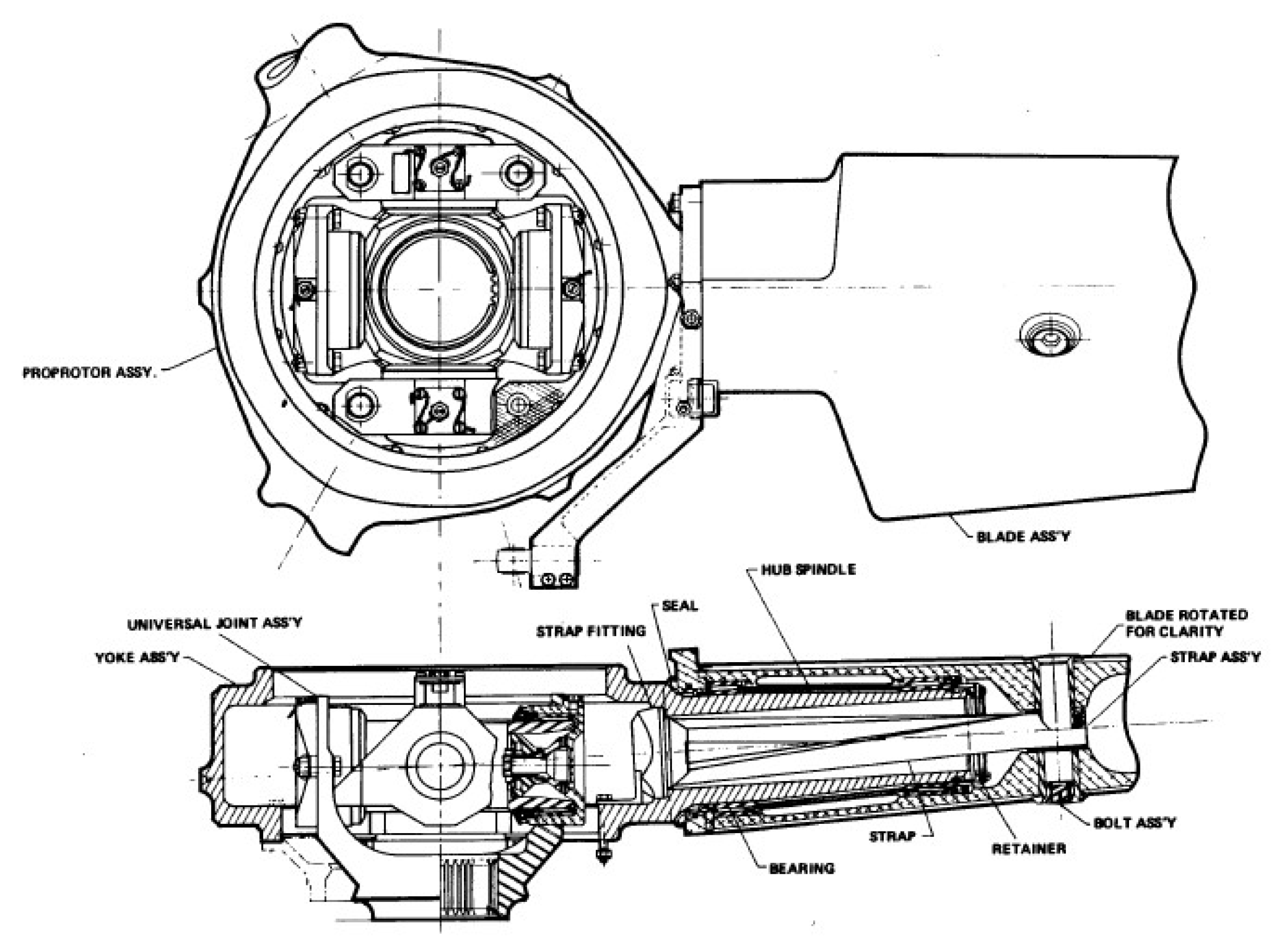
1.3. Gimballed Proprotors

Rotor Mathematical models of different levels of detail can be developed and the degree of complexity relates to the specific application. The specific case of tilt-rotor, however, requires some clarification: tilt-rotor aircraft generally makes use of gimballed proprotors (the name proprotor essentially comes from the combined propeller-rotor function this system provides in its operational range between helicopter and airplane mode). As reported in Reference [7], a gimballed rotor is basically a hingeless rotor attached to the rotor shaft through a gimbal, so the rotor head is able to tilt relative to the shaft with a mild elastic restraint and the hub tilt degree of freedom minimizes the blade flapping relative to the hub. As reported by Padfield in Reference [8] gimballed rotors generally use either a Universal joint or a constant velocity (homokinetic) joint. According to Reference [2], the XV-15 gimballed rotor exploits the Universal Joint principle (see Figure 1 and Figure 2).
In both cases, gimballed rotors present a substantial difference with respect to conventional articulated blade rotor systems, since if the elastic property of the blades is neglected, in gimballed rotors blade centrifugal forces are carried through the central hub structure and are balanced by the other blades, yielding to the suppression of the single blade flapping motion. However, the gimballed rotor does present a certain stiffness: the inner stiffness of the gimballed hub does provide a spring restraint and allows the torque transfer between the shaft and the blades but as reported by Carlson in Reference [7], the nature of the resulting fundamental stress and vibration is supposed to be reduced and advantageous with respect to conventional hinge-less or bearing-less rotors. Furthermore, the blades of a gimballed rotor are in truth not infinitely rigid, so the blades will also be able to slightly flap independently despite being constrained to the gimballed hub. Consequently, if the responses of an articulated and a gimballed 3 blades rotor to a cyclic swashplate input are compared, the reader shall expect the response of the gimballed rotor to show reduced yet not absolutely absent 1/rev blade flapping motion due to the structural flexibility of the blade constrained to the hub. Furthermore, the hub loads are expected to present a 3/rev oscillation, being each blade’s airloads a function of the azimuth position and being the overall hub loads the result of a summation of the loads of the 3 blades. Thus, in gimballed rotors oscillatory loads are not completely cancelled and several are the studies focusing on the development of control systems to mitigate the effect of those oscillation within the overall aeroelastic behaviour of the aircraft, among which are References [9,10]. The mathematical modelling of gimballed rotors has been addressed in the past and several fruitful models were produced to properly address the aeromechanic and aeroelastic design of such rotors, the author can refer to comprehensive mathematical models such as Johnson’s CAMRAD [11] as well as specific tilt-rotor studies such as References [7,12], yet the complexity of these models has always been limiting their performance and its applicability to real-time flight simulation. As Heffley duly discussed in 1988 in Reference [13] for the conventional helicopter case, if a minimum required level of complexity is to be defined, mathematical models for piloted flight simulation shall include an adequate representation of the main rotor dynamics to properly reproduce the hover as well as the forward flight characteristic modes of the rotorcraft. Among all the complex phenomena involved in the rotor dynamics, Heffley reckons that the coupling between the rigid-body modes and the rotor flapping does affect the handling qualities of the rotorcraft and that the flapping is most important to a pilot-in-the-loop simulation due to the characteristic control lag following cyclic input. Feathering and lead-lag dynamics are instead not mentioned in Reference [13] among the minimum set of dynamics to be included in a mathematical model for piloted simulations. However, while a Lead-Lag and Feathering dynamic formulations might be worth implementing in mathematical models for piloted simulations of conventional articulated rotors (an extensive model was developed by Takahashi in Reference [14] and could be revised for real-time applications), these additional dynamics are usually neglected for the tilt-rotor case, being proprotors generally considered stiff-in plane. As reported in the previous section of this paper, the baseline reference for tilt-rotor mathematical modelling for flight simulation used a simplified and static model of the proprotors flapping dynamics that made it suitable for piloted simulations with the software and hardware available at that time: while Reference [5] implemented a linearised static model of the proprotor disk flapping attitudes (lateral and longitudinal cyclic attitudes and conicity), Reference [6] introduces a first order dynamic model of the overall proprotors Tip Path Plane (TPP) flapping motion:
C 11 C 12 C 21 C 22 a ¯ ˙ 1 b ¯ ˙ 1 + A 11 A 12 A 21 A 22 a ¯ 1 b ¯ 1 = B 1 B 2 ,
where a ¯ 1 and b ¯ 1 are the longitudinal and lateral attitudes of the TPP, and decouples the coning dynamics reducing it to a static relation:
a 0 = 0.75 · T / n b + K β · a ¯ 0 I b · Ω ¯ 2 + K β ,
where T is the rotor thrust perpendicular to the disk plane, I b is the blade inertia, n b the number of blades, a ¯ 0 , the precone angle and Ω ¯ the non-dimensional rotor angular velocity. In Equation (1), the direct terms A 11 and A 22 of the stiffness matrix are influenced by the blades collective pitch, the rotor advance ratio and spring constant k G , which has a different value compared to k β in Equation (2), to account for the different spring characteristic of the gimbal and that of blade structure. The numerical values of k G and k β are reported in Table 1.
However, according to what reported by Ferguson in Reference [6], since the required solution time would have exceeded that allowable for the real-time simulation using the Sigma 8 computer located at NASA ARC, the dynamic flapping model was not implemented in the simulation and the blade flapping due to cyclic inputs is assumed to occur instantaneously considering the rotor in an equilibrium condition, yielding to Equation (3). As reported by Ferguson in Reference [6], the requirement for that model was to “keep the computational loop time to less 70 ms in order to maintain real-time” (p. 7), and the “differential equations for blade flapping that would properly account for the rotor following time were determined to require a solution time in excess of that allowable” (p. 12). The authors of the present paper assume that the limits of the model in Reference [6] were related to the hardware and software set up available back then in 1980, the use of the same model with updated hardware would in principle allow the use of the dynamic flapping model shown in Equation (1). However, the authors of the present paper were not able to fully reproduce Ferguson’s model only based on Reference [6], due to the lack of a complete description of the mathematical derivation and the unclear definition of some variables, as reported in Reference [15].
A 11 A 12 A 21 A 22 a ¯ 1 b ¯ 1 = B 1 B 2 .
Relatively more recent works generally reduce the flapping dynamics to that of the TPP as already introduced in Reference [6], modelled as a first-order system, or, like McVicair in Reference [16], implement a detailed modelling of the blades’ flapping motion which allows to include the 3/rev oscillations of the hub loads but treats the proprotor as articulated rather than gimballed. On the other hand, Padfield suggests in Reference [8] the FLIGHTLAB gimbal formulation, which neglects the first harmonic flapping and the coning due to the blades’ flexibility and only accounts for the overall gimbal motion.
In previous developments of their tilt-rotor model for real-time simulation, the authors of the present paper used the GTRS described in Reference [6] as baseline for the overall aerodynamic modelling of the generic tilt-rotor but replaced the reference rotor model with a novel one which uses a multi-blade formulation of the rotor’s airloads and flapping motion and tested it successfully in the Research and Didactics Simulator (ReDSim) of ZHAW, a reconfigurable flight simulation platform for both helicopters and airplanes. This rotor model exploits a second order semi-analytical formulation of the flapping motion of each blade of the rotor and it is reported here in Equation (4) in short form for the j-th blade, being m the inertial term, c the damping, k the stiffness of the flapping hinge and F β the external forcing input.
m β j ¨ + c β j ˙ + k β j = F β , j .
The terms in Equation (4) can be expressed as
m = I β c = M 1 k = M 2 + m b r cg a z 2 + K β F β = M 3 m b r cg ( a z 3 g z ) ,
where M 1 , M 2 , M 3 represent the aerodynamic moment resulting from the integration along the blade span, I β is the blade moment of inertia, m b is the blade mass, r cg is the distance of the centre of gravity of the blade from the origin of the hub reference system, g z is the acceleration of gravity and a z , 2 , a z , 3 z-components of the acceleration due to the blade motion in space (see next section for more details). Equation (4) is computed for each blade and the result fed back into the inflow and airloads computation. Forces and moments are computed for each blade and summed up at the origin of the hub reference system. As reported in Reference [15], tests performed on the multi-purpose rotor mathematical model showed good correlation with the experimental data in terms of overall hub forces and moments for both the XV-15 tilt-rotor and the UH-60 helicopter cases. However, the model in Reference [15] was essentially formulated as a fully-articulated rotor in which a spring component K β (see Equation (5)) in each blade’s flapping equation was introduced and tuned according to what reported in Reference [6] to better approximate the behaviour of a gimballed rotor. Therefore, this formulation in Reference [15] could not distinguish the stiffness of the gimbal, which influences the cyclic response of the proprotor, from the stiffness of each blade, which causes the rotor cone. As reported in Table 1, the stiffness of the gimbal is generally very small and tuned to provide adequate cyclic control of the rotor, therefore it is not strictly comparable to that of the metal blade-retention. The novel model presented in the following sections of this paper takes inspiration from the elegant and simple formulation of 2-bladed rotor flapping dynamics introduced by Chen in Reference [17] as well as the insightful descriptions of the gimbal rotors in Padfield’s work [8] and aims to modify the multi-articulated rotor formulation previously developed by the authors of Reference [15] to distinguish the contribution of the gimbal stiffness K G and that of K β associated to the elastic flapping of the blade and responsible for the coning of the rotor disk. While the extended formulation is described in the following sections of this paper, the resulting flapping equation can be written in rotating axis, for the j-th blade, as
m β j ¨ + c β j ˙ + c struct Δ β j ˙ + k β j + k G β G , j + k β Δ β j = F β , j ,
where m, c and F β are unchanged with respect to Equation (5), while c s t r u c t is an additional term accunting for the structural damping. β G represents the gimbal attitude in the rotating reference system and can be related to the overall β by the matrix B ψ , a linear combination of the blades’ azimuthal distance
β G = B ψ · β .
β now represents the overall angle between the blade and the plane perpendicular to the rotor mast (origin of the non-rotating reference system), while the actual blade flapping due to the blade elasticity and responsible of the disk coning is
Δ β = β β G .
This formulation is expected to better correlate with the dynamic response of the gimballed rotors without neglecting the elastic blade flapping motion and the resulting coning dynamics. Furthermore, the novel formulation allows the improvement of the response without overly increasing the complexity of the mathematical model and ensuring the real-time performance of the resulting Simulink code without making use of an expensive and less flexible hardware/software set up.

2. Mathematical Model

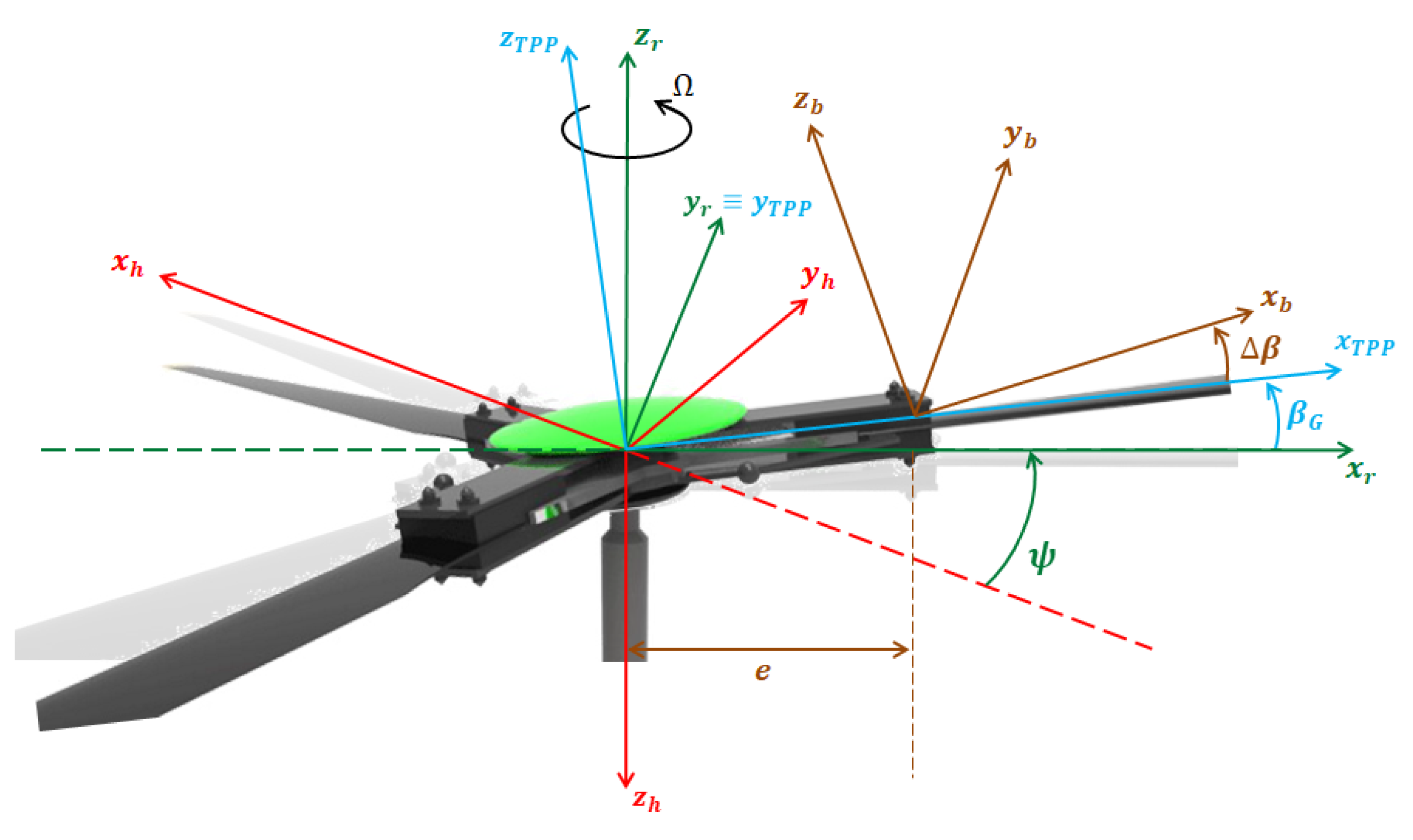
2.1. Reference Frames

The presence of a gimbal joint introduces an additional degree of freedom, so the set of reference systems used in Reference [15] and reported here in Figure 3 to describe the motion of an articulated rotor has been modified by adding a reference system which, according to the assumptions made later in Section 2.5, is aligned to the rotor tip-path-plane. The four reference frames are listed below.
Hub 
—Fixed, centered in the rotor hub, with:
  • x h in the hub plane and positive forward;
  • y h in the hub plane and positive outboard (starboard for the right rotor, port for the left rotor);
  • z h perpendicular to the hub plane and positive downwards.
Rotating 
—Centered in the rotor hub, rotating with angular speed equal to Ω , and having:
  • x r coincident with the projection of the blade axis on the hub plane and positive outwards;
  • z r perpendicular to the hub plane and positive upwards;
  • y r perpendicular to x r and z r (hence positive in the blade advancing direction).
Tip-path-plane (TPP) 
—Centered in the rotor hub, rotating about y r with angular speed equal to β ˙ G ; its axes are:
  • y t p p coincident with y r (perpendicular to the blade and positive in its advancing direction);
  • z t p p perpendicular to the rotor tip-path-plane and positive upwards.
  • x t p p perpendicular to y t p p and z t p p ;
Blade 
—Centered in the blade flapping hinge, rotating with angular speed equal to Δ β ˙ ; its axes are:
  • x b coincident with the blade axis and positive from the flapping hinge to the blade tip;
  • y b coincident with y t p p and y r (perpendicular to the blade and positive in its advancing direction);
  • z b perpendicular to x b and y b .
Transformations between different reference frames are obtained using the following rotation matrices:
  • From Blade system to TPP system:
    T Δ β = cos Δ β 0 sin Δ β 0 1 0 sin Δ β 0 cos Δ β = cos ( β β G ) 0 sin ( β β G ) 0 1 0 sin ( β β G ) 0 cos ( β β G ) ,
    where both β and β G are positive when the blade flaps upwards.
  • From TPP system to Rotating system:
    T β G = cos β G 0 sin β G 0 1 0 sin β G 0 cos β G
  • From Rotating system to Hub system:
    T ψ = cos ψ sin ψ 0 sin ψ cos ψ 0 0 0 1 ,
    where ψ = Ω t is the blade azimuth angle, that is, the angle between x r and the negative direction of x h , and is positive according to the direction of the rotor angular speed Ω (counter-clockwise for the right rotor, clockwise for the left rotor).

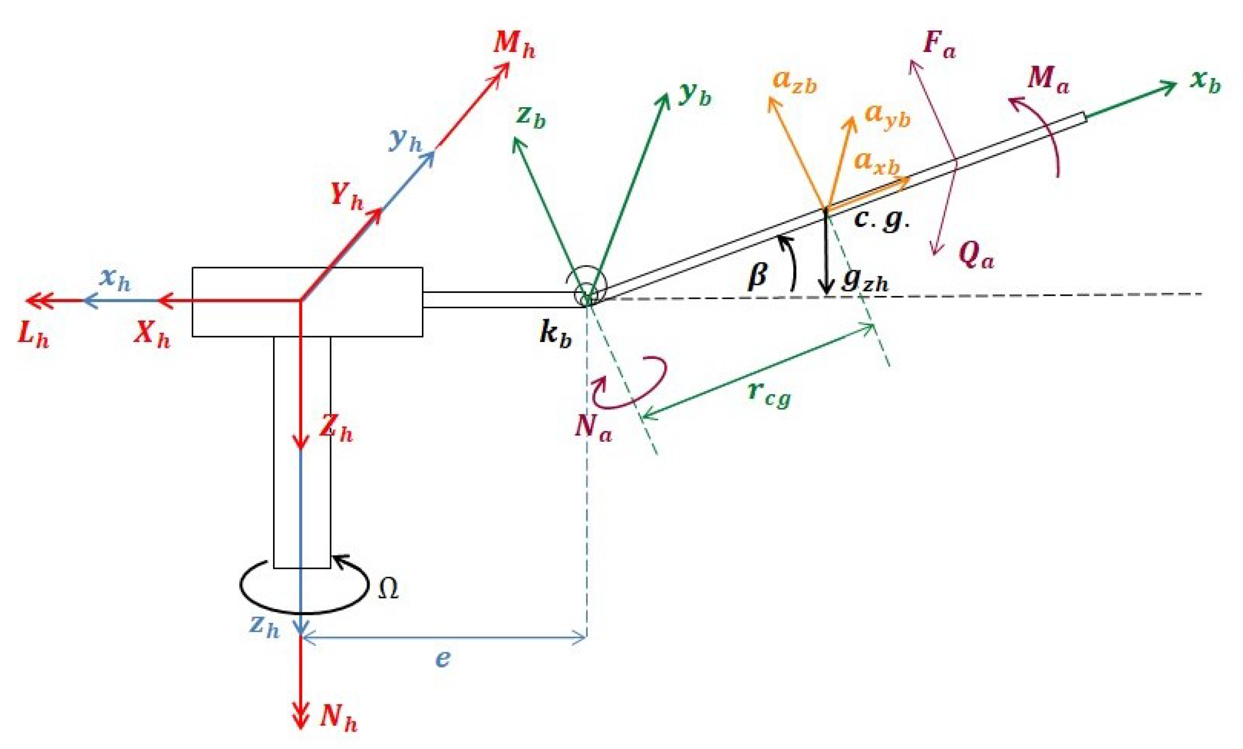
2.2. Blade Position, Speed and Acceleration

Position, speed and acceleration of a generic blade section S are determined with respect to the frames of reference defined in Section 2.5. The following vectors are defined, representing, respectively, the aircraft linear speed, linear acceleration, rotational speed and rotational acceleration, with respect to the Hub reference frame:
V h = u h v h w h ; a h = u ˙ h v ˙ h w ˙ h ; ω h = p h q h r h ; ω ˙ h = p ˙ h q ˙ h r ˙ h .
The position vector of the blade section in the Blade reference frame is
r S , b = r 0 0 ,
while the position of S in the TPP reference frame:
r S , t p p = T Δ β · r S , b + e 0 0 ,
where e is the flapping hinge offset. The speed of the blade section in the TPP reference frame is given by the following three contributions.
  • Relative speed of S with respect to the TPP system, due to blade rotation around the flapping hinge:
    V S , r e l , t p p = T Δ β · 0 Δ β ˙ 0 × r S , b .
  • Linear speed of the origin of the TPP system (due to aircraft motion):
    V t p p = T β G 1 · T ψ 1 · V h .
  • Tangential speed owing to reference frame rotation, which in turn is due to aircraft motion, gimbal motion and rotor spinning:
    V S , t a n g , t p p = ω t p p × r S , t p p ,
    where:
    ω t p p = T β G 1 · T ψ 1 · ω h + 0 β ˙ G 0 + 0 0 Ω .
Therefore, the total section speed in the TPP reference frame is expresse as
V S , t p p = V S , r e l , t p p + V t p p + V S , t a n g , t p p ,
while the velocity of the blade section in the blade system results in
V S , b = T Δ β 1 · V S , t p p .
The blade section acceleration in the TPP reference frame is given by the sum of the following five contributions:
  • relative acceleration of S (due to blade flapping) with respect to the TPP system, which in turn comprises a tangential and a centrifugal component:
    a S , r e l , t p p = T Δ β · 0 Δ β ¨ 0 × r S , b + 0 Δ β ˙ 0 × 0 Δ β ˙ 0 × r S , b ,
  • linear acceleration of the origin of the TPP system (due to aircraft motion):
    a t p p = T β G 1 · T ψ 1 · a h .
  • tangential acceleration owing to angular acceleration of the TPP reference frame:
    a S , t a n g , t p p = ω ˙ t p p × r S , t p p ,
    where:
    ω ˙ t p p = T β G 1 · T ψ 1 · ω ˙ h + 0 β ¨ G 0 + 0 0 Ω ˙
  • centrifugal acceleration, due to rotation of the TPP reference frame:
    a S , c e n t r , t p p = ω t p p × ω t p p × r S , t p p .
  • Coriolis acceleration:
    a S , C o r , t p p = 2 ω t p p × V S , r e l , t p p .
The resulting total blade section acceleration in the TPP system is:
a S , t p p = a S , r e l , t p p + a t p p + a S , t a n g , t p p + a S , c e n t r , t p p + a S , C o r , t p p .
Finally, the total acceleration in the Blade reference frame can be obtained as:
a S , b = T Δ β 1 · a S , t p p .

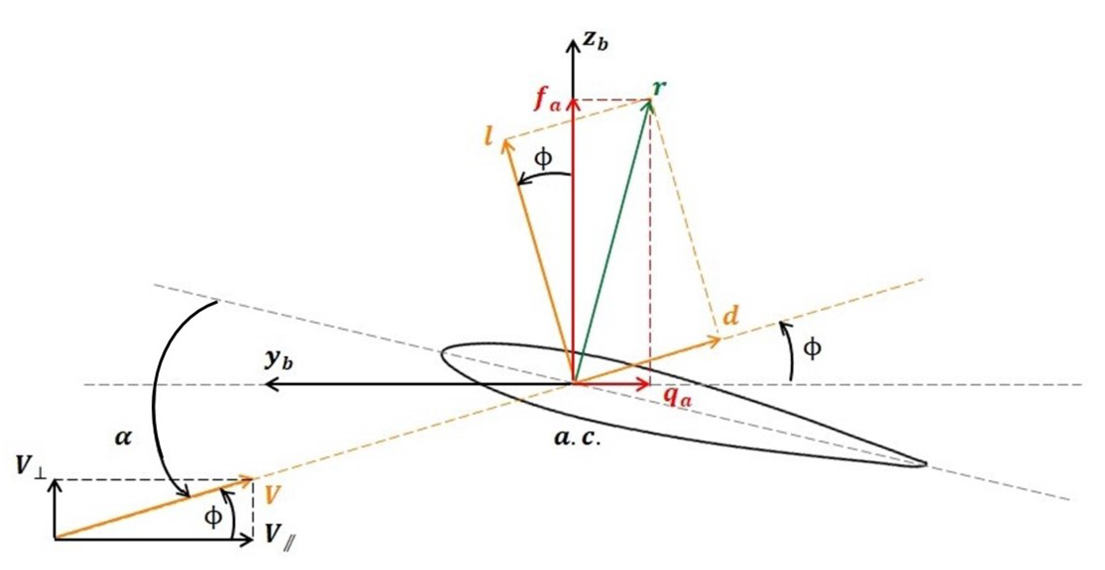
2.3. Rotor Aerodynamics

The blades airloads are modelled according to the Blade Element Theory as suggested in Reference [18]. Each rotor blade is divided into a finite number of sections, the aerodynamic loads being determined for each section and then integrated along the blade span. The aerodynamic forces generated by a generic blade section are represented in Figure 4.
Only lift and drag are considered in the present model, while the pitching moment about the aerodynamic centre is neglected. In order to compute the aerodynamic forces, the (absolute) angle of attack of each blade section must be determined:
α = ϑ twist + ϑ 0 A 1 cos ψ B 1 sin ψ K 1 β α 0 + ϕ ,
where:
  • ϑ twist is the twist angle, function of the position along x b ;
  • ϑ 0 , A 1 and B 1 are, respectively, the collective pitch, the lateral and the longitudinal cyclic;
  • K 1 = tan δ 3 , being δ 3 the pitch-flap coupling angle;
  • α 0 is the zero-lift angle of attack;
  • ϕ is the inflow angle.
The inflow angle identifies the direction of the airflow affecting the blade section, and can in turn be expressed as:
ϕ = arctan V V .
V is the component of the airflow speed, in wind axes, which is perpendicular to the blade section; to determine it, the following effects are taken into account:
  • blade motion V S , b ;
  • rotor inflow speed
    V inflow = Ω R λ 0 + r R λ 1 c cos ψ r R λ 1 s sin ψ ,
    in which the three inflow states λ 0 , λ 1 c and λ 1 s can be computed according to Pitt-Peters dynamic Model as described in Reference [19].
V is the component of the airflow speed, in wind axes, parallel to the blade section, for which only the blade motion V S , b [ 2 ] is taken into account. Both V and V are non-linear functions of β , β G , β ˙ and β ˙ G , thus making also ϕ and α non-linear functions of such quantities. Assuming small angles, it is possible to write:
sin β β ; sin β G β G ; and cos β 1 ; cos β G 1 .
Consequently, neglecting higher-order infinitesimals and considering the hinge offset to be null (the full derivation is not reported here for the sake of brevity), the expressions of V and V can be written as
V = B 1 x u o r λ 1 c Ω + q h r β u h cos ψ + + A 1 x u o r λ 1 s Ω + β v h + p h r sin ψ Ω R λ 0 r β ˙ + w h V = β p h r + v h cos ψ + β q h r + u h sin ψ r Ω + r h .
As a result of the linearisation all terms in β G and β ˙ G in Equation (32) disappear and two linear functions of only β and β ˙ are obtained. Moreover, these functions are identical to those derived in Reference [15] for an articulated rotor having hinge offset e = 0 . Since ϕ is itself a non-linear function of V and V , a linearisation is performed by means of a first-order Taylor expansion around the point ( β = 0 , β ˙ = 0 ) :
ϕ ( β , β ˙ ) ϕ ( β = 0 , β ˙ = 0 ) + ϕ β ˙ | β = 0 β ˙ = 0 β ˙ + ϕ β | β = 0 β ˙ = 0 β
Thus, the inflow angle becomes a linear function having the following form:
ϕ = ϕ 1 β ˙ + ϕ 2 β + ϕ 3
where:
ϕ 1 = n 1 d 3 n 3 2 + d 3 2 ϕ 2 = n 2 d 3 n 3 d 2 n 3 2 + d 3 2 ϕ 3 = arctan n 3 d 3
and
n 1 = r n 2 = u h cos ψ + v h sin ψ n 3 = ( B 1 x u o r λ 1 c ) Ω + r q h cos ψ + ( A 1 x u o r λ 1 s ) Ω + r p h sin ψ Ω R λ 0 + w h d 2 = r cos ψ p h sin ψ q h d 3 = cos ψ v h + sin ψ u h r ( r h Ω ) .
Equation (33) substituted into Equation (28), yields:
α = α 1 β ˙ + α 2 β + α 3
where:
α 1 = ϕ 1 α 2 = K 1 + ϕ 2 α 3 = ϑ twist + ϑ 0 A 1 cos ψ B 1 sin ψ α 0 + ϕ 3 .

2.4. Aerodynamic Forces and Moments

The blade section angle of attack being expressed according to Equation (28), if the airfoil lift and drag curves are known, lift and drag can be determined for each blade section. Since both C l and C d depend on α and the latter is a function of β and β ˙ , their expressions are linearised using a first-order Taylor expansion in the neighbourhood of ( β = 0 , β ˙ = 0 ) :
C l C l | β = 0 β ˙ = 0 + d C l d α α β ˙ | β = 0 β ˙ = 0 β ˙ + d C l d α α β | β = 0 β ˙ = 0 β = C l | β = 0 β ˙ = 0 + C l α | β = 0 β ˙ = 0 α 1 β ˙ + C l α | β = 0 β ˙ = 0 α 2 β
C d C d | β = 0 β ˙ = 0 + d C d d α α β ˙ | β = 0 β ˙ = 0 β ˙ + d C d d α α β | β = 0 β ˙ = 0 β = C d | β = 0 β ˙ = 0 + C d α | β = 0 β ˙ = 0 α 1 β ˙ + C d α | β = 0 β ˙ = 0 α 2 β .
Once ϕ , α and the aerodynamic coefficients are known, the aerodynamic forces can finally be computed. The lift and drag generated by each blade section are, respectively
d L = 1 2 ρ V 2 c C l d r ; d D = 1 2 ρ V 2 c C d d r ,
where V = V 2 + V 2 is the airflow speed. By projecting the lift and drag into the Blade reference frame, the following forces and moments are obtained:
  • aerodynamic force along z b :
    d F a = d D sin ϕ + d L cos ϕ = 1 2 ρ V 2 c ( C d sin ϕ + C l cos ϕ ) d r
  • aerodynamic force along y b :
    d Q a = d D cos ϕ d L sin ϕ = 1 2 ρ V 2 c ( C d cos ϕ C l sin ϕ ) d r ,
  • aerodynamic moment around y b :
    d M a = d F a r = 1 2 ρ V 2 c ( C d sin ϕ + C l cos ϕ ) r d r ,
  • aerodynamic moment z b :
    d N a = d Q a r = 1 2 ρ V 2 c ( C d cos ϕ C l sin ϕ ) r d r .
For implementation in the flapping dynamics equation, the terms in β and β ˙ in the expression of m a are collected as
d M a = d M 1 β ˙ + d M 2 β + d M 3 ,
with:
d M 1 = 1 2 ρ V 2 c ( C d α ( α 3 ) sin ϕ + C l α ( α 3 ) cos ϕ ) α 1 r d r d M 2 = 1 2 ρ V 2 c ( C d α ( α 3 ) sin ϕ + C l α ( α 3 ) cos ϕ ) α 2 r d r d M 3 = 1 2 ρ V 2 c ( C d ( α 3 ) sin ϕ + C l ( α 3 ) cos ϕ ) r d r .
The overall aerodynamic loads generated by each blade (as shown in Figure 5) are subsequently obtained by integrating the above forces and moments along the whole length of the blade:
F a = 0 R d F a ; Q a = 0 R d Q a ; M a = 0 R d M a ; N a = 0 R d N a
M 1 = 0 R d M 1 ; M 2 = 0 R d M 2 ; M 3 = 0 R d M 3 ;
Integration along the blade is operated symbolically, using the method of the trapezoids. Let d F be a generic aerodynamic load generated by a blade section, and n the number of intervals in which the blade has been divided; the length of each interval is designated as Δ x . The overall aerodynamic load generated by the blade is then:
F = 0 R d F Δ x 2 d F ( x 1 ) + 2 d F ( x 2 ) + 2 d F ( x 3 ) + + 2 d F ( x n ) + d F ( x n + 1 ) .

Airfoil Aerodynamic Coefficients

As the blades of a tilt-rotor aircraft proprotors operate in a wide range of angles of attack, the complete airfoil polar curves (i.e., for angles of attack spanning from 180 to + 180 degrees) need to be included in the model inizialization file. Available data for the NACA 64-208 airfoil covered only a limited range of angles of attack; therefore, the missing parts of the polar curves have been reconstructed using the empirical approach described hereafter.
  • The airfoil lift and drag coefficients are expressed by tables that are function of the angle of attack while for ranges of angle of attack outside available data the approximation proposed by Hoerner in Reference [20] is used:
    C l = k C l sin α cos α C d = k C d sin α 2 ,
    where the coefficients k C l and k C d are tuned to match the reference data in Reference [21].
  • The missing portions of the polar curves are determined using Equation (46), and introducing corrections in order to best fit the available aerodynamic data.
  • The derivatives of the aerodynamic coefficients with respect to the angle of attack ( C l α and C d α ) are computed using the centred difference method:
    f ( x j ) f ( x j + 1 ) f ( x j 1 ) x j + 1 x j 1 .

2.5. Flapping Dynamics Model for Gimballed Rotors

Instead of explicitly modelling the gimbal dynamics and increasing the complexity of the existing model, the kinematic constraint on the blades is taken into account by introducing the following two assumptions:
  • The flapping angle of each blade is computed by adding to the gimbal attitude, β G , another contribution Δ β , representing the variations of flapping angle in each of the N blades due to the blade flexibility or to a coning hinge:
    β j = β G j + Δ β j j = 1 , , N .
  • The gimbal plane is assumed to be parallel to the rotor tip-path-plane, hence:
    β G j = β 1 s sin ψ j + β 1 c cos ψ j j = 1 , , N ,
  • the angles β 1 s and β 1 c in Equation (49) are the lateral and longitudinal attitudes of the TPP and are obtained using the multi-blade coordinate transformation (MBC) truncated to the first order, therefore
    β 1 s = 2 N j = 1 N β j sin ψ j ; β 1 c = 2 N j = 1 N β j cos ψ j .
Strictly speaking, the second hypothesis would be verified only if Δ β was identically null. However, the approximation is reasonably acceptable when considering that the coning stiffness of the XV-15 rotor hub is in the order of 10 5 Nm/deg (Reference [6]). Evaluating β G for each blade, and substituting in its expression the definitions of the multi-blade coordinates, the following matrix is obtained:
β G 1 β G 2 β G N = 2 N 1 cos ( ψ 2 ψ 1 ) cos ( ψ N ψ 1 ) cos ( ψ 1 ψ 2 ) 1 cos ( ψ N ψ 2 ) cos ( ψ 1 ψ N ) cos ( ψ 2 ψ N ) 1 β 1 β 2 β N ,
which can be written in compact form as
β G = B ψ · β
and where
B ψ i , j = 2 N cos ( ψ j ψ i ) i , j = 1 , , N .
Since the azimuth angle for each blade is given by
ψ j = Ω t + ( j 1 ) 2 π N j = 1 , , N
the following can be written:
B ψ i , j = 2 N cos ( j i ) 2 π N i , j = 1 , , N .
Consequently, β G is here related to the overall blade flapping angle β through a matrix whose coefficients are constant in time and depend only on the number of blades. In an analogous way,
β ˙ G = B ψ · β ˙ .
The flapping dynamics equation for each blade is written in the following form:
m β ¨ + c β ˙ + c struct Δ β ˙ + k β + k G β G + k β Δ β = F β
where:
  • m, c and F β are
    m = I β c = M 1 F β = M 3 m b r cg ( a z 3 g z ) .
  • k contains the contributions of aerodynamic and inertial loads to system stiffness:
    k = M 2 + m b r cg a z 2 .
    In a generic flight condition, k, c and F β are in general different for each blade.
  • c struct takes into account the system structural damping. As evaluating the structural damping is extremely difficult, it is a common practice to express this term as a function of other system parameters. In the present model, c struct has been expressed as a function of the viscous equivalent critical damping ratio, following the formulation proposed in Reference [22]:
    c struct = 0.3 · 2 m k β m .
  • k G contains the contributions to system stiffness dependent on β G :
    k G = k G + m b r cg a z G ,
    where k G is the torsional stiffness of the gimbal joint and a z G is z-component of acceleration seen by the blade due to the gimbal motion, function of the angular speed of the rotor Ω and the yaw rate of the rigid body, in hub axes, r h
    a z G = Ω Ω + r h r cg .
  • k β can represent either the stiffness of the hub coning hinge (if present), or the structural stiffness.
By substituting Δ β = β β G and Equation (52) in the flapping dynamics equation, and rewriting everything in matrix form, an equation in the following form is obtained:
M β ¨ + C β ˙ + K β = F β .
In which the following terms appear:
  • mass matrix:
    M = I β I
    where I is the identity matrix.
  • damping matrix:
    C = C a + c struct ( I B ψ ) ,
    with:
    C a = C a 1 0 0 0 C a 2 0 0 0 C a N C a j = M 1 j .
  • Stiffness matrix:
    K = K a + k β I ( k β k G ) B ψ ,
    with:
    K a = K a 1 0 0 0 K a 2 0 0 0 K a N K a j = M 2 j + m b r cg a z 2 j .
  • Non-homogeneous term:
    F β = F β 1 F β 2 F β N F β j = M 3 j m b r cg ( a z 3 j g z j ) ,
where M 1 j , M 2 j , M 3 j , a z 2 j , a z 3 j are computed for the j-th blade using Equations (44) and (27), while g z j is the gravity acceleration along z b for the j-th blade. For a three-bladed rotor such as the XV-15 one, in particular, B ψ reduces to:
B ψ = 2 3 1 3 1 3 1 3 2 3 1 3 1 3 1 3 2 3
and Equation (63) becomes
I β 0 0 0 I β 0 0 0 I β β ¨ 1 β ¨ 2 β 3 ¨ + 1 3 3 c 1 + c struct c struct c struct c struct 3 c 2 + c struct c struct c struct c struct 3 c 3 + c struct β ˙ 1 β ˙ 2 β 3 ˙ + + 1 3 2 k G + 3 k 1 + k β k β k G k β k G k β k G 2 k G + 3 k 2 + k β k β k G k β k G k β k G 2 k G + 3 k 3 + k β β 1 β 2 β 3 = F β 1 F β 2 F β 3 .
The dynamic problem is thus described by a system of second-order differential equations in which the only states are the flapping angles of each blade, and their derivatives.

2.6. Hub Loads

The loads transmitted by each rotor to the airframe constitute the main output of the rotor model. The following components are considered:
  • aerodynamic loads;
  • blade inertia;
  • blade weight;
  • forces and moments generated by the flapping hinge.
Once all forces and moments acting on each single blade are determined, the constraint reactions in the flapping hinge can be computed as
R = F ext m b a cg F int ,
where F ext denotes the external loads (i.e., those related to aerodynamics and gravity), F int indicates the internal loads produced by the flapping hinge, and a cg is the acceleration of the blade center of gravity. Due to Newton’s third law of motion, the loads transmitted by the blade to the rest of the aircraft, in the Blade reference frame, are simply:
F = R .
Subsequently, the vector F obtained for each blade is transported to the center of the rotor hub and referred to the Hub frame of reference. Eventually, the overall hub loads are computed by summing up contributions from each blade (namely X h , Y h , Z h , L h , M h , N h ).

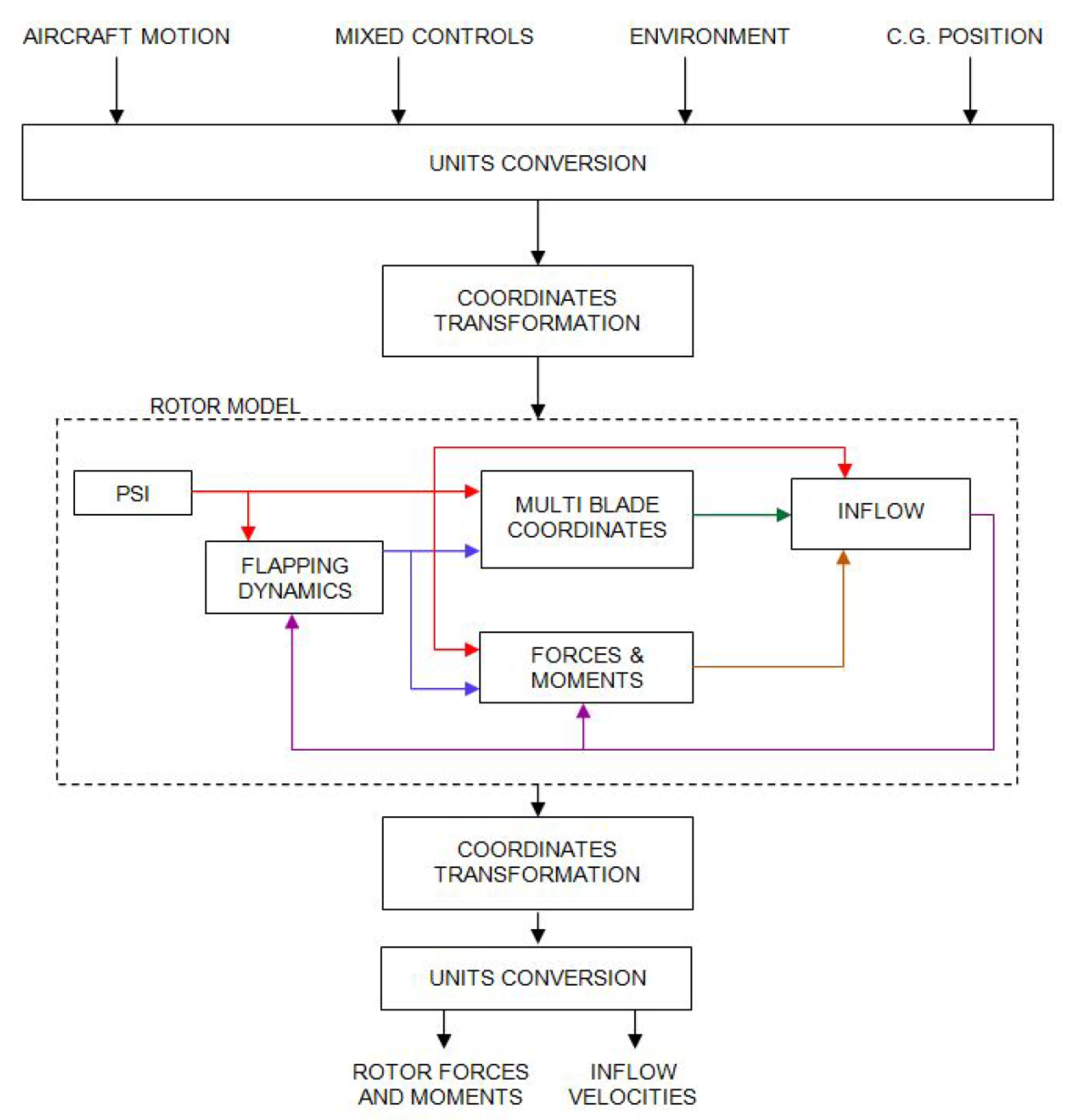
3. Software Implementation

3.1. Tilt-Rotor Simulation Model

The novel model of the flapping dynamics of the gimballed rotor is meant to be part of the comprehensive tilt-rotor mathematical model for real-time flight simulation developed by ZHAW and Politecnico di Torino and implemented in the Research and Didactics Simulator (ReDSim). The comprehensive model has already been introduced in Reference [15] and for the sake of brevity will not be described in detail again in this paper. The tilt-rotor model is developed in Simulink environment and structured in functional blocks accounting for the main components of the aircraft. The novel gimballed rotor model replaces the previous one within the overall model and no major modification to the code are needed. This structure allows to easily introduce new features in the Simulink code and run the new version on the simulator right away with no need for compilation and upload of any embedded software features on dedicated hardware. According to the tilt-rotor configuration, the rotor model is implemented twice in the model, once for the right rotor, once for the left one, being all variable of interest duly transformed from body to rotor reference systems accounting for the nacelle conversion angle.

3.2. Numerical Integration

The mathematical model of the rotor is meant to be implemented in Simulink in discrete form. The integration of the flapping dynamics Equation (63) is performed using a fourth-order Runge-Kutta solver:
y n + 1 = y n + 1 6 k 1 + 2 k 2 + 2 k 3 + k 4 ,
with:
k 1 = h f ( t n , y n ) k 2 = h f t n + h 2 , y n + k 1 2 k 3 = h f t n + h 2 , y n + k 2 2 k 4 = h f ( t n + h , y n + k 3 )
where h corresponds to the simulation sampling time T s . The current implementation uses a fixed sampling rate of 400 Hz for the numerical solution of flapping dynamics equations. As a matter of fact, the numerical stability of the solver is related to the high natural frequency of the blade flapping motion, which is affected by the great stiffness value K β (see Table 1). The fourth-order Runge-Kutta was found to ensure the correct solution of the equations using a sampling rate for which the hardware/software set-up used, can ensure soft real-time. On the other hand, the equations of motion of the aircraft as well as the rotors’ inflow dynamics can be integrated using a discrete Euler backwards method with a constant sampling rate of 400 Hz as well.

3.3. Stand-Alone Model

In order to evaluate the behaviour of the gimballed rotor model and compare it to that of the articulated one, a Simulink model was created to simulate an isolated rotor, mounted on a test rig and subject to the desired external condition (in terms of air density and airstream velocity components) and the desired inputs (in terms of collective, lateral cyclic and longitudinal cyclic blade pitch inputs). A flow chart of the stand-alone rotor model architecture is provided in Figure 6.

4. Results and Discussion

The standalone model was used to compare the response of the previous rotor model (articulated version) and the proposed one, the novel gimballed rotor model. The reference rotor geometry is the XV-15 rotor for both the model options and all data was derived from References [2,6]. Results are presented below in this section.

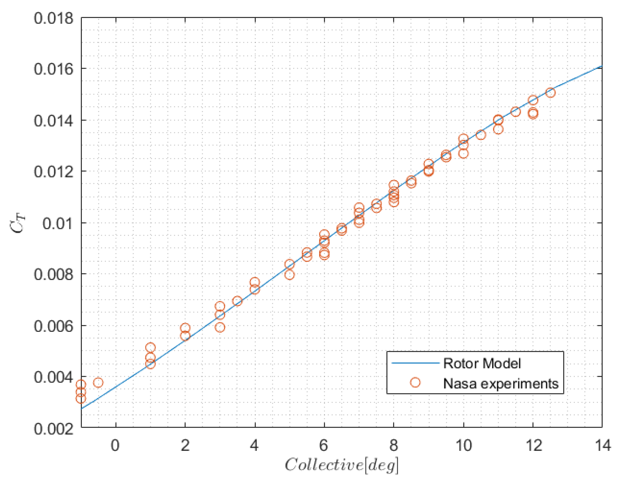
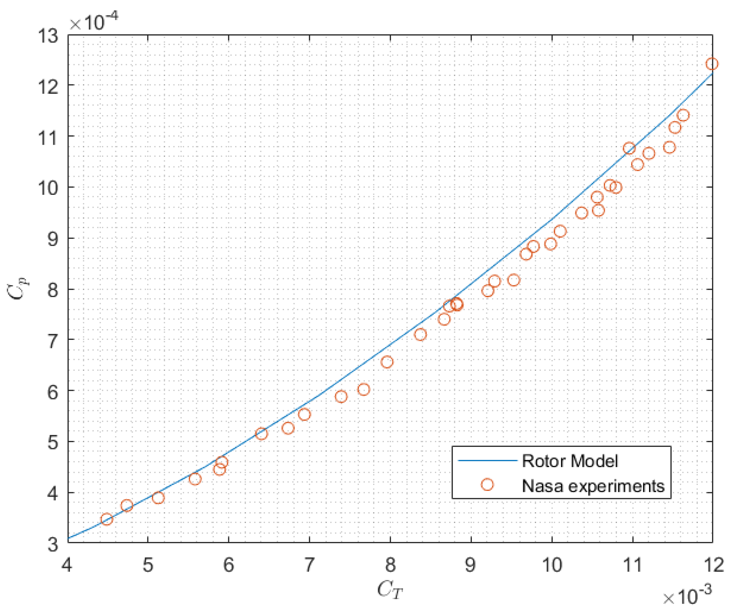
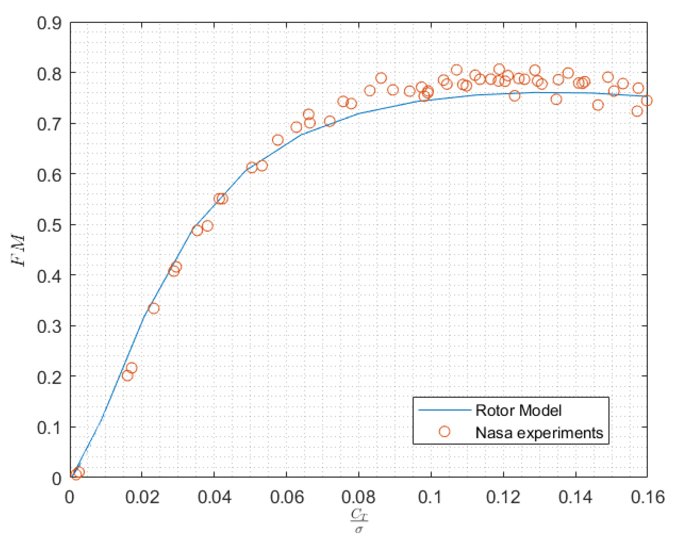
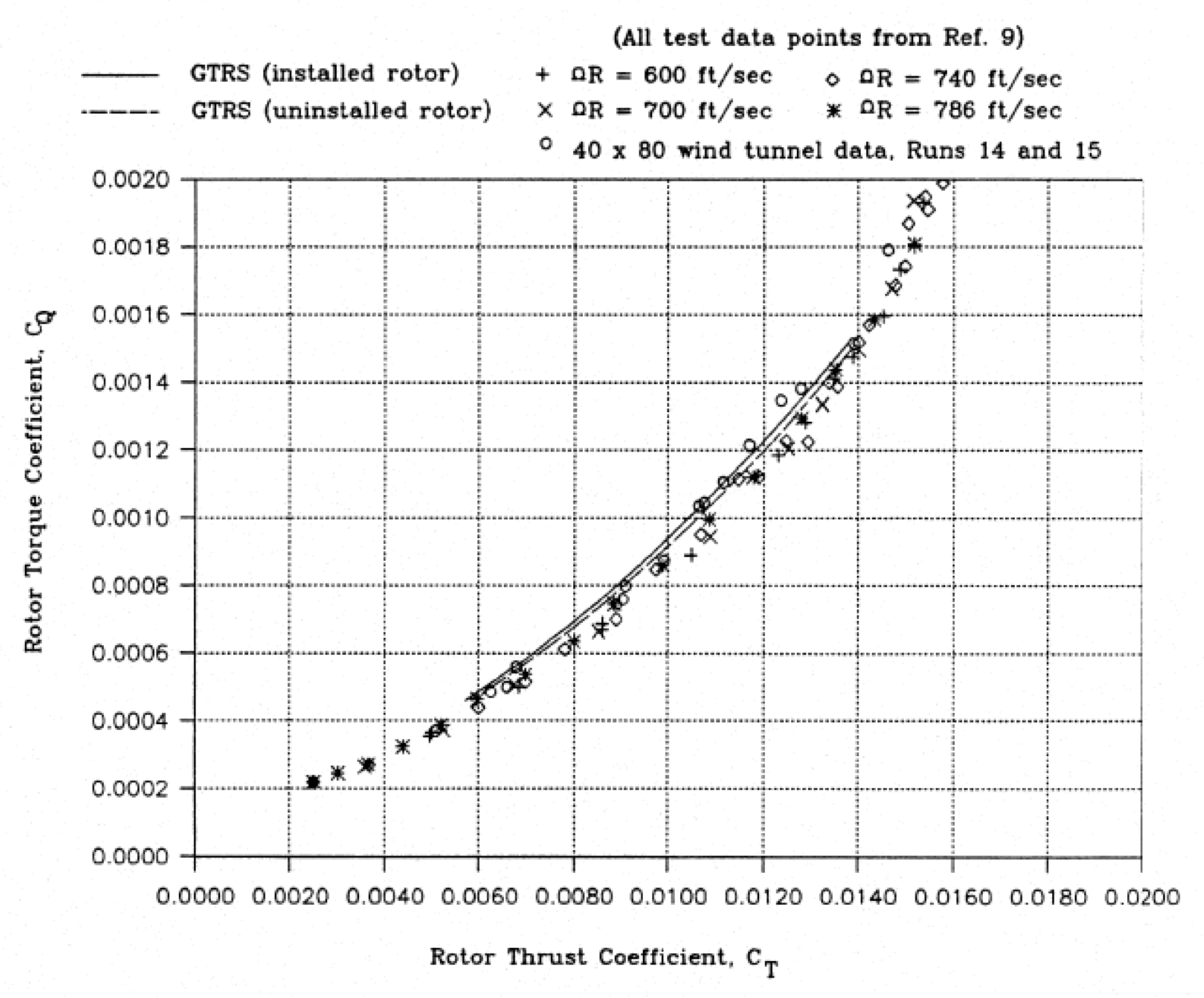
4.1. Rotor Performance

The proposed gimballed rotor model was compared with the available data in terms of thrust coefficient C T , power coefficient C P and Figure of Merit F M . The reference data is derived from the experimental test conducted by NASA on the isolated XV-15 Proprotor and reported in Reference [21]. As shown in Figure 7, the model matches the experimental data for the thrust coefficient very closely, while Figure 8 shows that the power coefficient is slightly over-predicted at high thrust values. As a result the predicted figure of merit (see Figure 9) is slightly lower than what experimentally registered, as well. However, as shown in Figure 10, the results of the proposed rotor model in terms of static thrust and power coefficient of the uninstalled rotor, match what predicted by the reference model and validated against experimental wind tunnel data in Reference [6] The results, however, show a good correlation with the experimental data and further improvements can be made with a finer tuning of the airfoil’s aerodynamic parameters.

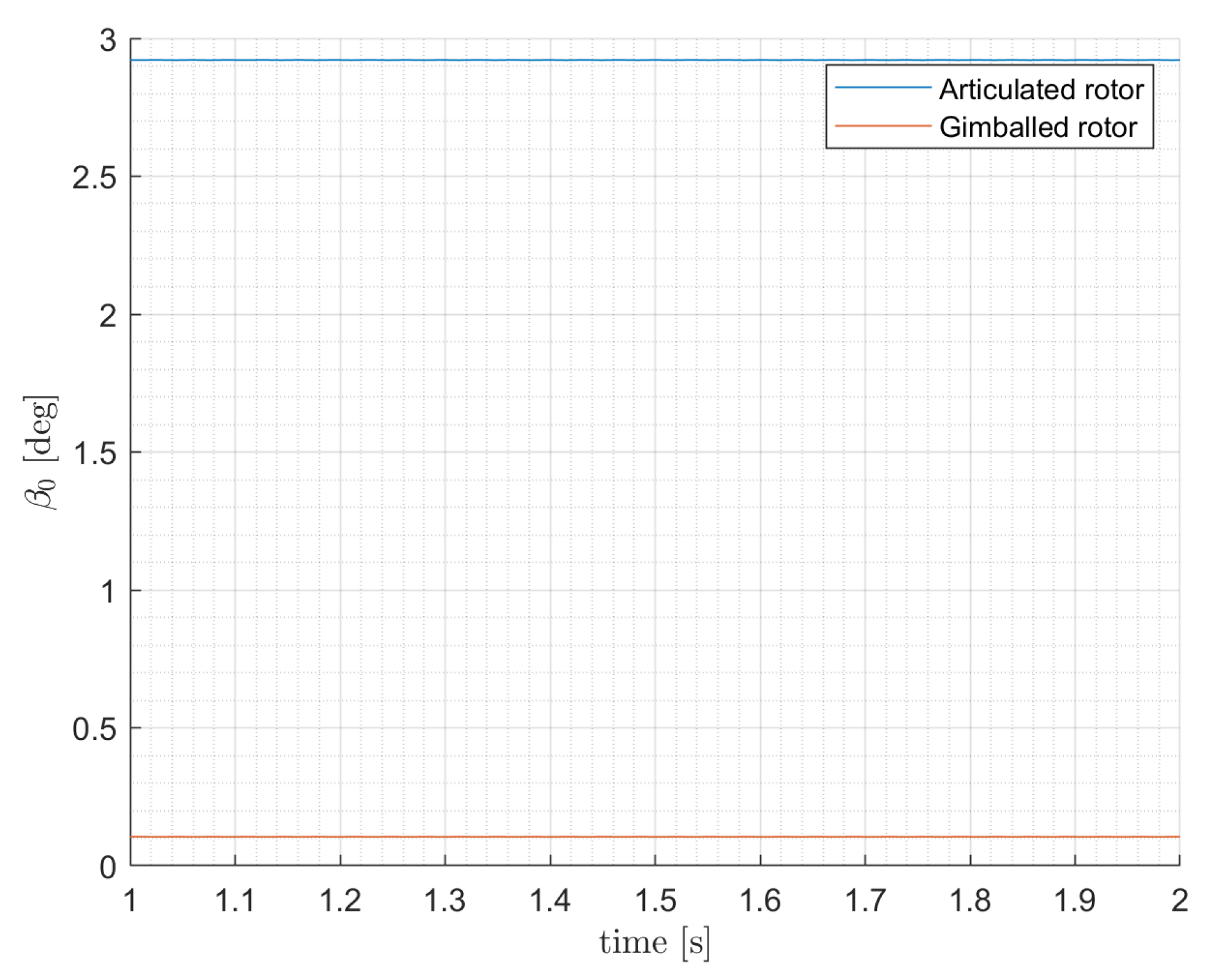
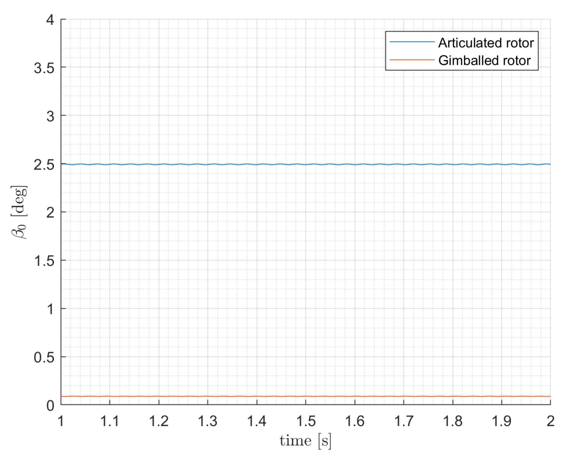
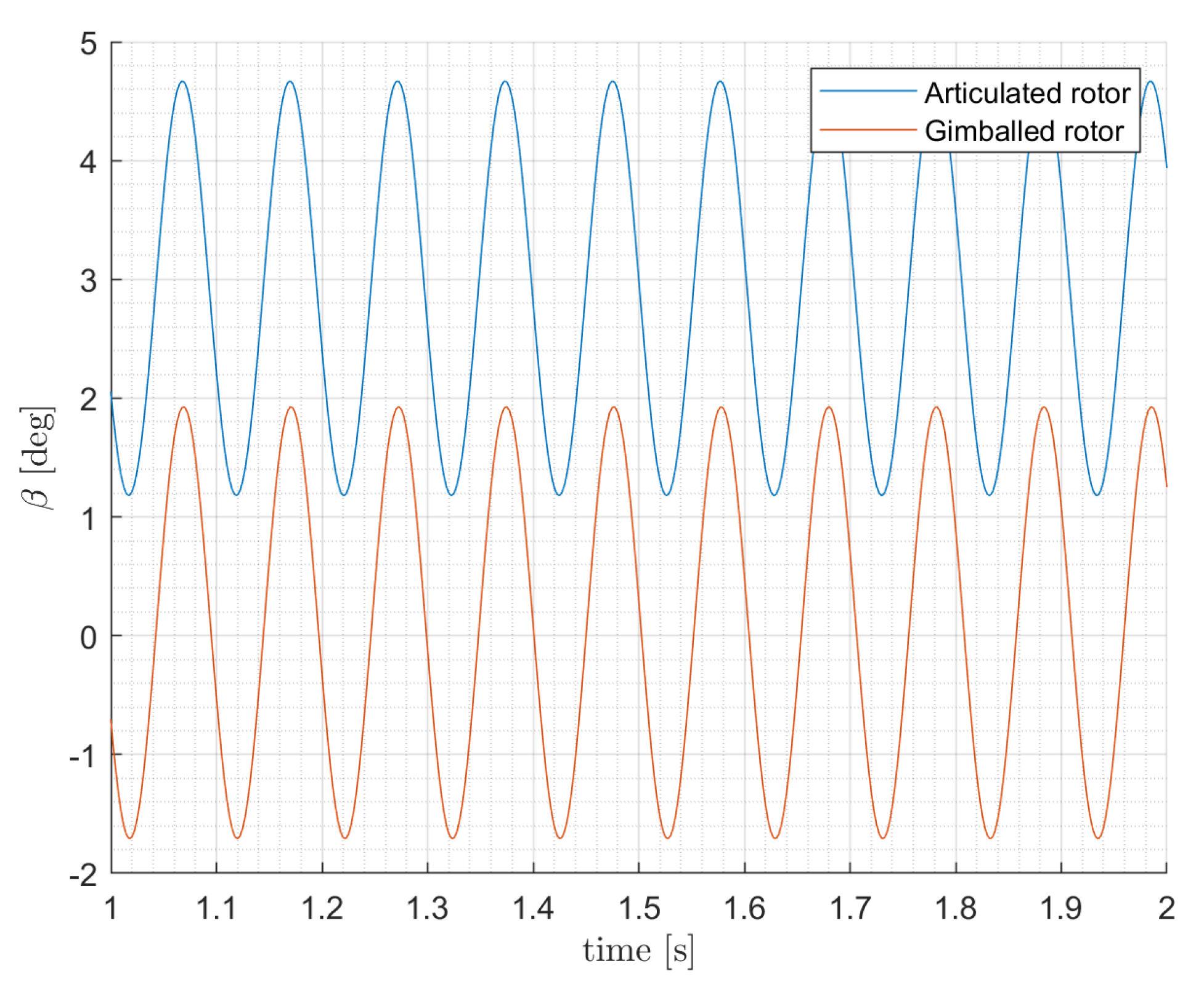
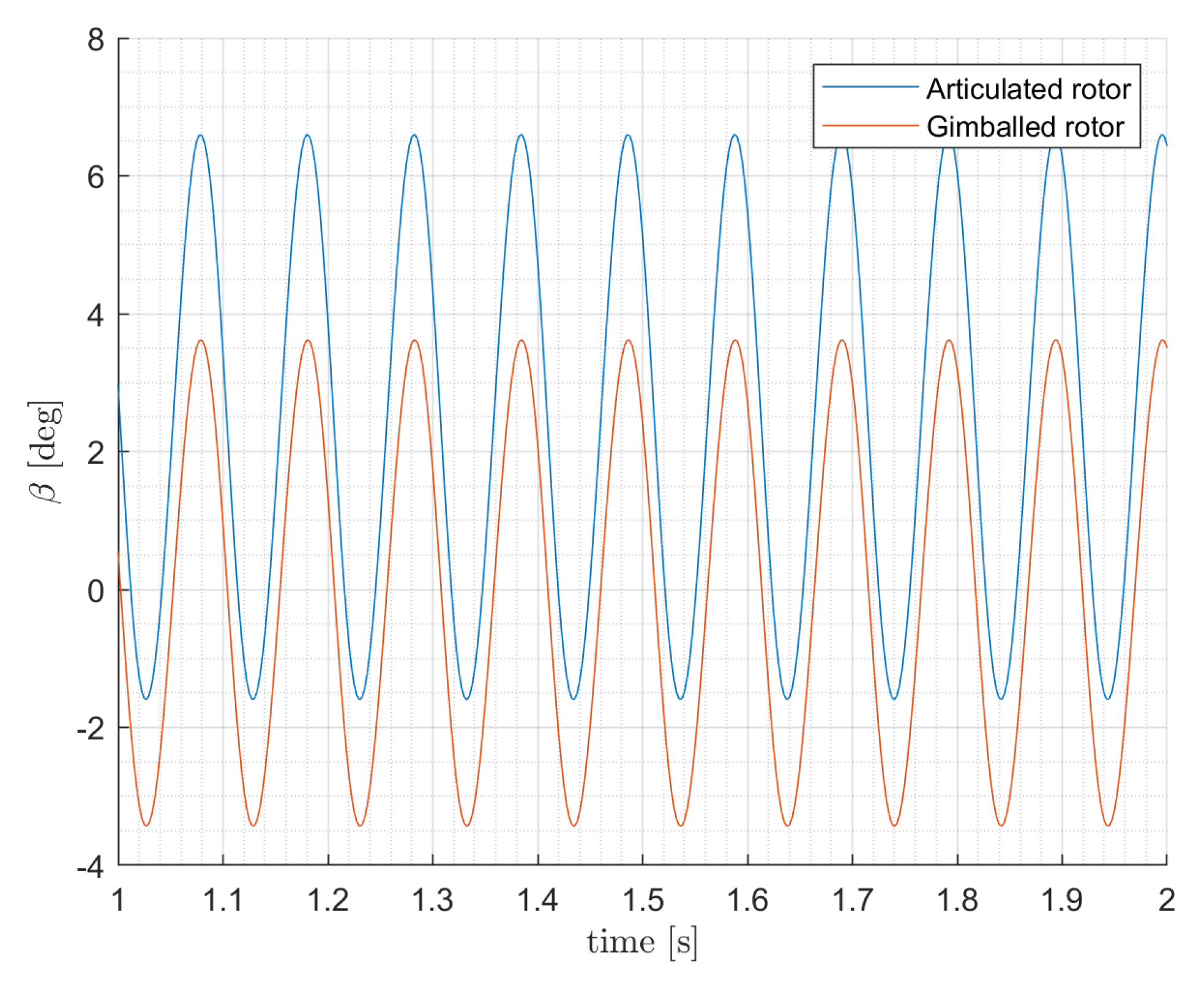
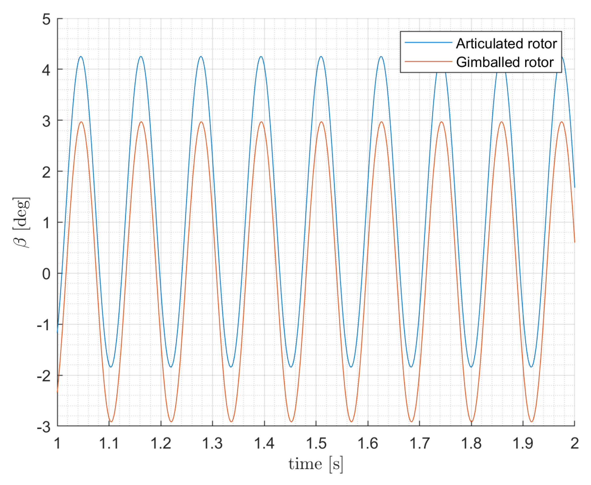
4.2. Blades Flapping Motion and Disk Coning

Here below the time histories of the flapping motion of the rotor blades are reported, for three different conditions:
  • Hover
  • Low-speed flight in helicopter mode
  • High-speed flight in airplane mode
For the sake of brevity, only the overall flapping angle β of the j-th blade of the rotor and the resulting coning angle β 0 (relative to the sole flapping motion and not accounting for the rotor pre-cone angle) are reported, to prove the thesis of this study. The input parameters are reported in Table 2 and are derived from the trim values of the overall tilt-rotor model in those three specific conditions.
The results are compared with those of the previous version of the model (articulated rotor version). As clearly shown in Figure 11, Figure 12 and Figure 13, the novel gimbal model behaves as expected, therefore a considerable reduction of the coning angle is experienced, if compared to the behaviour of the previous rotor model (articulated version), in virtue of the effect of K β . The coning angle β 0 is obtained averaging the flapping of the N blades of the rotor around 1 revolution. Precisely, for the sake of clarity Figure 14, Figure 15 and Figure 16 show the flapping motion of the single j-th blade, but the other two blades would shown the same motion, with a different phase angle, due to the different azimuthal position. Accordingly, the Simulink stand-alone model is run for each condition, the results are collected in the Matlab workspace and processed with a Matlab script to produce the plots. What reported here below are the time histories of the responses of interest for 1 s of simulation, in which the initial second is omitted not to account for the transient and only show the resulting stabilised response.

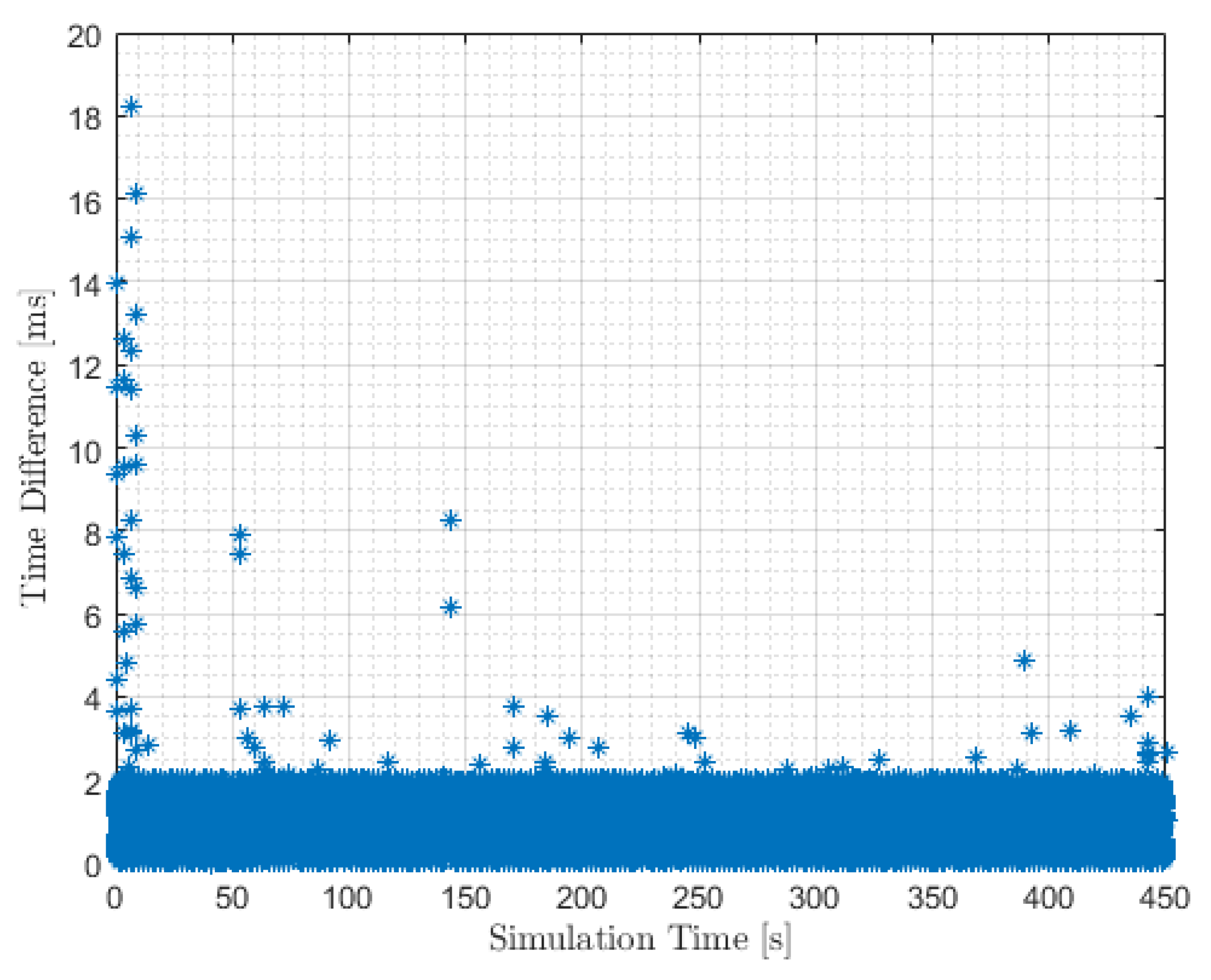
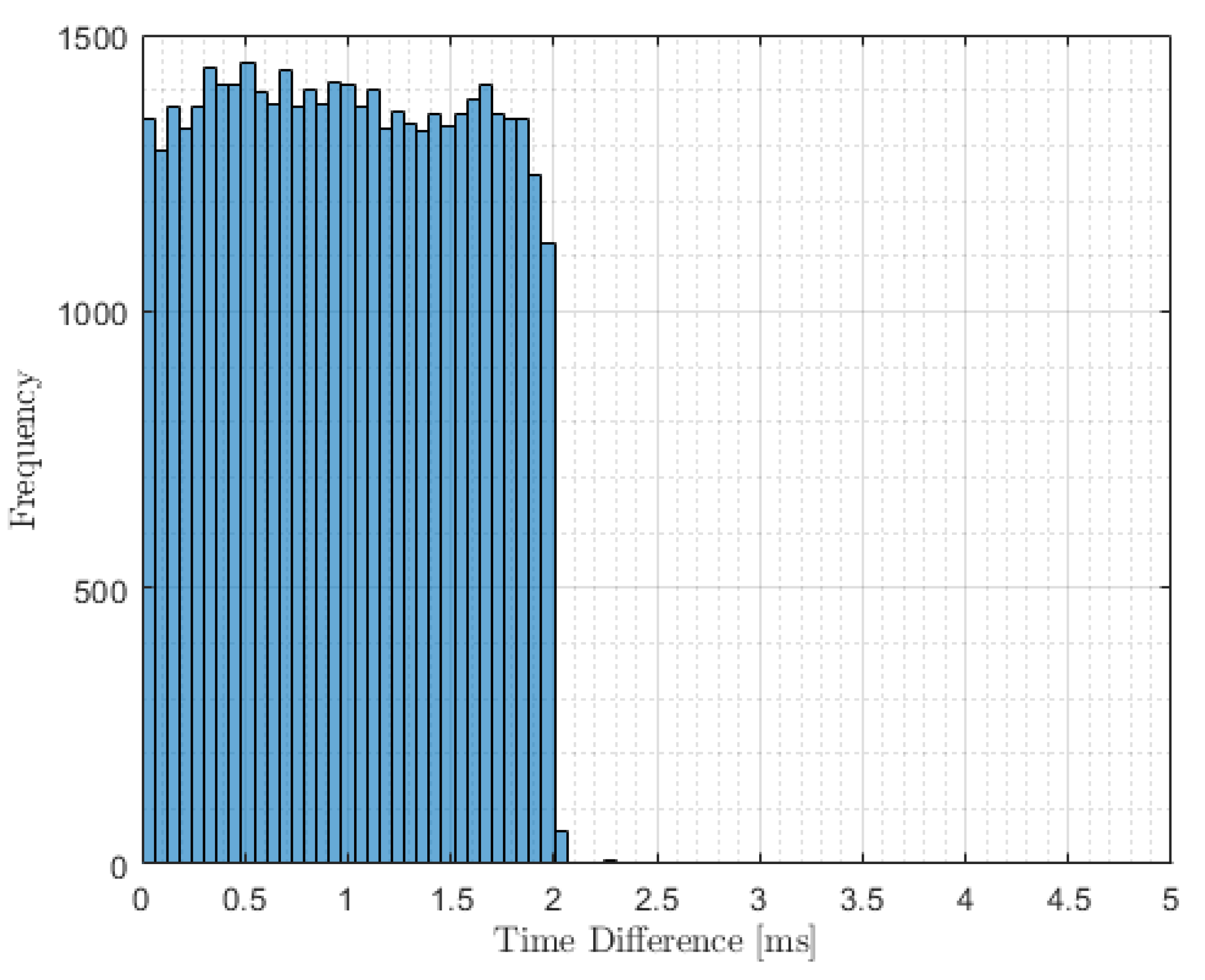
4.3. Code Performance in Pilot-In-The-Loop Simulations

The proposed rotor model was implemented in the comprehensive tilt-rotor model and tested in the ReDSim at ZHAW. The overall Flight Simulation Platform and has been described in Reference [15] and no major changes were introduced, except the replacement of the previous rotor model with the new proposed one. To allow pilot-in-the-loop simulations, the Simulink® model must be able to maintain real-time. This is done with a proprietary C++ S-Function that, for each iteration step, compares the time of the simulation with the time of the computer. For this particular test, the S-Function was called at 400 Hz (every 2.5 ms) and the difference between simulation time and real-time was registered. The data is reported here in Figure 17. The histogram of the time difference in Figure 18 shows that about 99.87% of the samples have less than 2.5 ms of time difference. The mean value of the distribution will also depend on the resolution of the function used to suspend the execution of the current thread until the time-out elapses. This is deemed to be acceptable for pilot-in-the-loop simulation, where the main requirement is represented by the time delay between the pilot input and aircraft response (as per “Allowable airplane response delay” in MIL-F-8785C). The time history in Figure 17 shows a few peaks of values greater than 2.5 ms, one reaching 18 ms. These peaks are assumed to be caused by other services that are running on the Windows computer and will be investigated in the future. Several mitigations are possible such as: removal of windows services, stop antivirus at run time, increase task priority, and so forth. It is obvious from Figure 18 that the execution of one iteration of the model can be achieved in less than 2.5 ms, since the simulation is always able to recover from a delay caused by the operating system.

5. Conclusions and Future Developments

Based on the baseline offered by Ferguson in Reference [6] about the GTRS, a novel, more detailed and efficient model was developed. Compared to the reference, the novel model introduces a higher order flapping dynamic formulation, it accounts for the gimbal constraint to the blades flapping motion, it exploits a dynamic modelling of the rotor’s inflow and offers a more detailed multi-blade description of the rotor’s air-loads. As shown in the previous section of this paper, the novel mathematical formulation allows to increase the accuracy of the results (compared to the previous articulated version of the model) without overly increasing the complexity of the model or compromising its real-time capability. Thus, the novel gimballed rotor mathematical model improves the previous rotor model and the comprehensive tilt-rotor flight simulator of ZHAW and Politecnico di Torino, which can now be used for extensive tilt-rotor piloted simulations, from helicopter mode, through conversion mode to airplane mode. The novel mathematical formulation is believed to offer additional insights in the tilt-rotor real-time simulation topic as well as a new baseline for the development of other models for different aircraft architectures. However, the authors acknowledge that due to the lack of data on the actual coning angles of the XV-15 rotors, a comparison against experimental data could not be performed at this time. Future works will involve an extensive review of the aerodynamic database of the tilt-rotor simulation model aiming for a more complete validation against available data of the XV-15, as well as handling qualities studies performed in the ReDSim and flight control systems research and development activities. Precisely, an extensive handling qualities assessment will be performed according to ADS-33 as well as specific tilt-rotor-based MTEs, as suggested by Padfield in Reference [8]. Eventually, further studies involving tilt-rotor inceptor architectures are envisaged such as combined Collective-And-Throttle-Lever solutions.

Author Contributions

Conceptualization, F.B., P.C. and G.G.; methodology, F.B. and P.C.; software, A.A., F.B. and P.C.; validation, A.A. and F.B.; formal analysis, A.A., F.B.; investigation, A.A. and F.B.; resources, F.B., G.G. and P.C.; data curation, A.A.; writing—original draft preparation, F.B.; writing—review and editing, A.A., P.C. and G.G.; visualization, A.A. and F.B.; supervision, G.G. and P.C.; project administration, G.G. and P.C.; funding acquisition, G.G., P.C. All authors have read and agreed to the published version of the manuscript.

Funding

This research received no external funding.

Acknowledgments

This activity is part of a Doctoral Research Program (Ph.D. in Aerospace Engineering at Politecnico di Torino) and a Master Degree Thesis (M.Sc. in Aerospace Engineering at Politecnico di Torino) supported by Zurich University of Applied Sciences, Centre for Aviation.

Conflicts of Interest

The authors declare no conflict of interest.

References

  1. Anderson, S.B. Historical Overview of V/STOL Aircraft Technology; NASA TM81280; NASA: Washington, DC, USA, 1981.
  2. Harris, F.D. NASA/SP-2015-21259 Vol III. In Introduction to Autogyros, Helicopters, and Other V/STOL Aircraft; National Aeronautics and Space Administration: Washington, DC, USA; Ames Research Center: Mountain View, CA, USA; Moffet Field: Santa Clara, CA, USA, 2015; pp. 16–40. [Google Scholar]
  3. Maisel, M.D.; Giulianetti, D.J.; Dugan, D.C. NASA SP-2000-4517. In The History of the XV-15 Tilt Rotor Research Aircraft: From Concept to Flight; The NASA History Series; National Aeronautics and Space Administration, Office of Policy and Plans, NASA History Division: Washington, DC, USA, 2000. [Google Scholar]
  4. Rosenstein, H.; McVeigh, M.A.; Mollenkof, P.A. V/STOL Tilt Rotor Aircraft Study Mathematical Model for a Real Time Simulation of a Tilt Rotor Aircraft (Boeing Vertol Model 222); NASA: Washington, DC, USA, 1973; Volume VIII.
  5. Harendra, P.B.; Joglekar, M.J.; Gaffey, T.M.; Marr, R.L. V/STOL Tilt Rotor Study Volume V. A Mathematical Model For Real Time Flight Simulation of the Bell Model 301 Tilt Rotor Research Aircraft; Final Report; CR114614; NASA: Washington, DC, USA, 1973.
  6. Ferguson, S.W. A Mathematical Model for Real-Time Flight Simulation of a Generic Tilt-Rotor Aircraft; NASA CR166536; NASA: Washington, DC, USA, 1988.
  7. Carlson, R.G.; Miao, W.-L. Aeroelastic Analysis of the Elastic Gimbal Rotor; NASA CR166287; NASA: Washington, DC, USA, 1981.
  8. Padfield, G.D. Helicopter Flight Dynamics, including a treatment of Tiltrotor Aircraft, 3rd ed.; John Wiley & Sons: Hoboken, NJ, USA, 2018. [Google Scholar]
  9. Mattaboni, M.; Masarati, P.; Quaranta, G.; Mantegazza, P. Multibody Simulation of Integrated Tiltrotor Flight Mechanics, Aeroelasticity, and Control. J. Guid. Control. Dyn. 2012, 35, 5. [Google Scholar] [CrossRef]
  10. Nixon, M.W.; Kvaternik, R.G.; Settle, T.B. Tiltrotor Vibration Reduction Through Higher Harmonic Control. In Proceedings of the American Helicopter Society 53rd Annual Forum, Virginia Beach, VA, USA, 29 April–1 May 1997. [Google Scholar]
  11. Johnson, W. CAMRAD/JA A Comprehensive Analytical Model of Rotorcraft Aerodynamics and Dynamics; Johnson Aeronautics Version; User’s Manual: Palo Alto, CA, USA, 1988; Volume II. [Google Scholar]
  12. Barkai, S.M.; Rand, O.; Peyran, R.J.; Carlson, R.M. Modeling and Analysis of Tilt-Rotor Aeromechanical PhenomenaIn. Math. Comput. Model. 1998, 27, 17–43. [Google Scholar] [CrossRef]
  13. Hefflex, R.; Mnich, M.A. Minimum-Complexity Helicopter Simulation Math Model; NASA: Washington, DC, USA, 1988.
  14. Takahashi, M.D. A Flight-Dynamics Helicopter Mathematical Model with a Single Flap-Lag-Torsion Main Rotor; NASA TM102267; NASA: Washington, DC, USA, 1990.
  15. Barra, F.; Godio, S.; Guglieri, G.; Capone, P.; Monstein, R. Implementation of a Comprehensive Mathematical Model for Tilt-Rotor Real-Time Flight Simulation. In Proceedings of the 45th European Rotorcraft Forum, Warsaw, Poland, 17–20 September 2019. [Google Scholar]
  16. McVicair, J.; Scott, G. A Generic Tilt-Rotor Simulation Model with Parallel Implementation. Ph.D. Thesis, University of Glasgow, Glasgow, Scotland, 1993. [Google Scholar]
  17. Chen, R.T.N. Effects of Primary Rotor Parameters on Flapping Dynamics; NASA TP-1431; NASA: Washington, DC, USA, 1980.
  18. Johnson, W. Helicopter Theory; Dover Publications, Inc.: Mineola, NY, USA, 1980. [Google Scholar]
  19. Chen, R.T.N. A Survey of Nonuniform Inflow Models for Rotorcraft Flight Dynamics and Control Applications; NASA TM 102219; NASA: Washington, DC, USA, 1989.
  20. Hoerner, S.F. Fluid Dynamic; Lift, S.F., Ed.; Hoerner Fluid Dynamics: Brick Township, NJ, USA, 1975. [Google Scholar]
  21. Harris, F.D. Hover Performance of Isolated Proprotors and Propellers—Experimental Data; NASA CR 219486; NASA: Washington, DC, USA, 1988.
  22. Bielawa, R.L. Rotary Wing Structural Dynamics and Aeroelasticity, 2nd ed.; AIAA American Institute of Aeronautics and Astronautics: Reston, VA, USA, 2006. [Google Scholar]
  23. Ferguson, S.W. Development and Validation of a Simulation for A Generic Tilt-Rotor Aircraft; NASA CR166537; NASA: Washington, DC, USA, 1989.
Figure 1. Scheme of the working principle of the hub universal joint (Reference [2]).
Aerospace 07 00124 g001
Figure 2. The XV-15 hub and blade-retention assembly (Reference [2]).
Aerospace 07 00124 g002
Figure 3. Reference frames for the right rotor.
Aerospace 07 00124 g003
Figure 4. Sketch of a generic blade section.
Aerospace 07 00124 g004
Figure 5. Simplified scheme of a rotor with the forces and moments acting on each blade.
Aerospace 07 00124 g005
Figure 6. Flowchart of the stand-alone rotor model.
Aerospace 07 00124 g006
Figure 7. Rotor hover performance—Variation of the thrust coefficient with the collective pitch.
Aerospace 07 00124 g007
Figure 8. Rotor hover performance—Power coefficient versus thrust coefficient.
Aerospace 07 00124 g008
Figure 9. Rotor hover performance—Figure of Merit ( F M = C T 3 / 2 / C P ) versus Thrust-to-solidity ratio.
Aerospace 07 00124 g009
Figure 10. Uninstalled Rotor—Power and Thrust Coefficient comparison between wind tunnel tests and Generic Tilt Rotor Simulator (GTRS) results, Reference [23].
Aerospace 07 00124 g010
Figure 11. Hover condition 1—time history of the resulting coning angle β 0 of the rotor.
Aerospace 07 00124 g011
Figure 12. Helicopter condition 2—time history of the resulting coning angle β 0 of the rotor.
Aerospace 07 00124 g012
Figure 13. Airplane condition 3—time history of the resulting coning angle β 0 of the rotor.
Aerospace 07 00124 g013
Figure 14. Hover condition 1—time history of the overall flapping angle β of the j-th blade.
Aerospace 07 00124 g014
Figure 15. Helicopter condition 2—time history of the overall flapping angle β of the j-th blade.
Aerospace 07 00124 g015
Figure 16. Airplane condition 3—time history of the overall flapping angle β of the j-th blade.
Aerospace 07 00124 g016
Figure 17. Time history of the time difference between simulation and computer time.
Aerospace 07 00124 g017
Figure 18. Histogram of the time difference between simulation and computer time.
Aerospace 07 00124 g018
Table 1. XV-15 blade and gimbal stiffness values.
ElementSimbolUnitValueReference
blade k β [ N m / deg ]244,047.23 [6]
gimbal k G [ N m / deg ]305.05 [6]
Table 2. Simulation input parameters for the three analysed conditions.
ElementSymbolUnitCond. 1Cond. 2Cond. 3
True Air SpeedTAS[ kts ]060180
Nacelle Angle i N [ deg ]90900
Rotor Angular speed Ω [ rpm ]589589517
Hub Inlet X-Velocity u h [ m / s ]030.359−2.998
Hub Inlet Z-Velocity u h [ m / s ]0−5.359−92.551
Collective pitch input (after mixing unit) θ 0 [ deg ]6.984.8228.26
Longitudinal cyclic pitch input (after mixing unit) B 1 [ deg ]−1.7830.2621.500

