Abstract
Designing a reconfiguration system for an aircraft requires a good mathematical model of the object. An accurate model describing the aircraft dynamics can be obtained from system identification. In this case, special maneuvers for parameter estimation must be designed, as the reconfiguration algorithm may require to use flight controls separately, even if they usually work in pairs. The simultaneous multi-axis multi-step input design for reconfigurable fixed-wing aircraft system identification is presented in this paper. D-optimality criterion and genetic algorithm were used to design the flight controls deflections. The aircraft model was excited with those inputs and its outputs were recorded. These data were used to estimate stability and control derivatives by using the maximum likelihood principle. Visual match between registered and identified outputs as well as relative standard deviations were used to validate the outcomes. The system was also excited with simultaneous multisine inputs and its stability and control derivatives were estimated with the same approach as earlier in order to assess the multi-step design.
1. Introduction
It is no doubt that flight safety is an issue of great importance in modern aviation and each risk should be reduced if possible. Thus, a lot attention is paid and numerous analyses are performed for each part of the design process e.g., in manufacturing [1], cockpit design [2,3], human-object interaction in terms of involuntary aircraft pilot interaction [4,5] or comfort assessment [6,7] and flight mechanics [8,9,10]. However, it still may happen that an adverse event occurs and it influences the flight safety.
Flight management systems are used in modern aircraft in order to limit pilot workload and thus raise the safety level. This approach allows to reduce human errors, however it introduces a new category of adverse events—control systems failures [11]. Detailed procedures and technical inspections limit the risk, but it still may occur and, in consequence, influence the flight safety. A common way of overcoming this issue in aviation is to use redundancy.
Unfortunately, including backup components and systems in the aircraft increases its mass, mechanical complexity, and reduces the available space, so it limits the object capabilities and performance [12]. It makes it impossible to use this approach for selected aircraft, including small unmanned aerial vehicles. For those objects, a different method must be selected in order to reduce the effects of the control system failure—reconfiguration.
The Flight Management System is the onboard aircraft system that uses navigational information, performance data, and flight parameters primarily to manage the flight plan. It is integrated with the autopilot and flight control systems and thus allows e.g., to reduce pilot workloads and limitations when controlling the aircraft. When aircraft is to be reconfigured the flight management system and autopilot use the fully operating system components to overcome the breakdown and finish the mission e.g., by returning to the base or continuing the task if this does not degrades the mission effectiveness significantly. The role of the flight management system and autopilot in this process depends on the particular system design e.g., flight controls reallocation can be performed by the flight management system, so it provides modified inputs for the autopilot after a failure was diagnosed or the autopilot receives the information as to which inputs are not available and it performs the controls reallocation itself. The primary aim of the reconfiguration is to eliminate effects of the system failures; however, it may also be used in order to gain tactical advantage during air combat or for investigations performed in in-flight simulators. The reconfiguration is performed either by using flight controls that are not used in the particular flight phase [13,14], by modifying control laws [15,16,17,18] or by readjusting the mission plan [19,20]. In each of those approaches a valid mathematical model is required.
Accurate models describing aircraft dynamics can be obtained from system identification [21,22,23,24,25]. This requires performing multiple experiments in which flight controls are used to excite aircraft motion. The experiments are performed during flight tests. The flight controls are separately deflected to provide that sufficient amount of diverse information about the object dynamics is stored in the measured flight data. It raises the cost of the experiments, in particular, when the object has multiple flight controls, so, e.g., in the case of an aircraft that uses multiple flight surfaces for reconfiguration, even if the controls are exciting the motion with respect to the same primary axis. To solve this issue, it is possible to design special manoeuvres that allow for simultaneous excitations by using multi-step [26] and multisine inputs [21,27], and this is preferable over exciting single surface separately. As the models are obtained from the data gathered during the experiment (i.e., identification is not performed in near real time), the time required to design the inputs should not be of a great concern.
In this paper, a system identification experiment design for a reconfigurable unmanned aerial vehicle with multiple flight controls is presented. The structure of the document is as follows. In Section 2, the aircraft under test and its simulation model are presented. In Section 3, the multi-step inputs are shown. For the flight controls that can be deflected simultaneously, a genetic algorithm was used to design those inputs. For the flight surfaces that were deflected once at a time, only the Marchand method was used to design the excitations. In Section 3, multisine inputs corresponding to multi-step manoeuvres are shown. The inputs that are presented in Section 3 and Section 4 were used to excite the aircraft simulation model shown in Section 2 and the response of the model was registered. On the basis of the registered data, the system was identified by using the output error method presented in Section 5 separately for multi-step and multisine manoeuvres. The results of the parameter estimation are shown in Section 6. The paper finishes with a short summary of conclusions.
The novelty of the paper is the design of the D-optimal multi-step multi-axis inputs for an aircraft with independent deflections of flight controls that usually work in pairs (e.g., ailerons). The D-optimal multi-step multi-axis excitations were already presented in [26], where the controls were deflected conventionally (e.g., left and right elevator parts were deflected with the same angle and in the same direction) for a simulation model of a large transport aircraft. As the paper presents the design that used flight controls that work in different way, for an object with different dynamics and was validated in flight (application results presented in [14]) it can be viewed as extension of the mentioned study. The multi-axis multisine manoeuvre is presented in the study in order to evaluate how good is the D-optimal design. The Multiplex Cularis UAV aircraft was selected because of the overall project objectives. In the case of large scale aircraft the cost would be increased and the risk could be not acceptable, as the overall project aim was the aircraft control system synthesis under high risk circumstances.
2. Model
System identification experiments were designed for the Multiplex Cularis aircraft that is presented in Figure 1. The aircraft is remotely controlled and a ground station can be used to excite the object from preprogrammed input signals. The technical data of the aircraft are shown in Table 1.
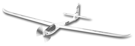
Figure 1.
Cularis aircraft [28].

Table 1.
Technical data.
In the conventional design, control surfaces of the aircraft are symmetrical to the longitudinal plane and work in pairs in order to ease the control and limit the system complexity. Here, as the flight controls were to enable reconfiguration, it was possible to excite each of them separately. Thus, in the study, seven flight controls deflections were defined: left and right aileron ( and ), left and right flap ( and ), left and right elevator part ( and ), and rudder (). The positive flight control deflections were for aileron, flap or elevator part deflected downwards and when rudder was deflected to the left.
Mathematical Model
A mathematical model of the aircraft was built in order to design the system identification experiments. Equations motion were derived in body axes system . The reference frame is presented in Figure 2. The origin of the coordinate system was located at the aircraft center of gravity O. The axis lies in the symmetry plane and is parallel to mean aerodynamic chord. The axis is directed toward right wing and the complements the right-handed coordinate system, thus pointing downwards. The system is related to frame through attitude angles (bank angle), (pitch angle), and (yaw angle). The coordinate system is carried by the aircraft, but its attitude is not changing—its parallel to Earth fixed coordinate system .
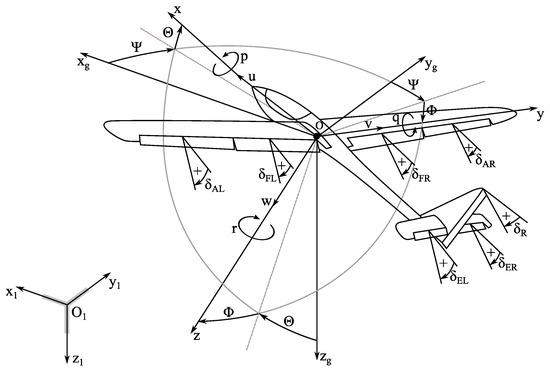
Figure 2.
Coordinate system, state, and control variables.
To develop equations of motion, the aircraft was modelled as a rigid body with vertical symmetry plane. Thus, from Newton second law of motion, the following equations were obtained [29]:
where u, v, and w are longitudinal, side, and vertical velocity, p, q, and r are roll, pitch, and yaw rates, and are bank and pitch angles, X, Y and Z are aerodynamic force components, L, M, and N are aerodynamic moment components, m stands for mass, g for gravitational acceleration, dot symbol denotes a derivative with respect to time, and 0 subscript refers to the value in equilibrium.
The set of equations was complemented by including kinematic relationships between attitude angles and angular rates [29]:
The linear aircraft model allows for accurately capturing dynamic properties and shortening the optimization time in simultaneous multi-step excitations design. This assumption is typically valid in major part of the flight envelope as can be seen e.g., in [25] and it is also reflected by the aeronautical standards referring to flight dynamics and control [30,31]. Thus, the nonlinear model was linearized. Small perturbations theorem was used for that purpose. Aerodynamic loads were expressed by using first order Taylor series approximation. In the equilibrium (trim point), the aircraft was flying 16 m/s at angle of attack 0.7354 deg at 30 m. The elevator deflection for both parts was 1.2314 deg and the throttle was set to 0.45. The trim point was calculated using the nonlinear model.
The model was expressed in state space form:
The state matrix A was composed of state matrices for longitudinal and lateral states:
The control matrix B contained matrices for longitudinal motion and lateral motion when the flight surfaces are deflected conventionally (i.e., in pairs). The deflection of the right and left flight control results in the same effect for longitudinal forces and moments, thus the index referring to the flight control position (right or left surface) was omitted in the control matrices (e.g., ). For the lateral-directional motion, a negative effect is produced for the corresponding flight controls, so a minus sign was included in the control matrices (e.g., ).
The control matrix also contained components that describe the influence of a single lateral-directional flight control on longitudinal motion and a single longitudinal flight control on lateral-directional motion :
The state vector consisted of linear velocity components, angular rates, and attitude angles:
and the control vector was containing flight controls deflections perturbations from the trimmed values:
Acceleration components were included in the outputs in order to raise the accuracy of the system identification performed later:
3. Multi-Step Inputs
Multi-step signals are among the most popular inputs in aircraft system identification due to their ease in application and robustness [22,23,32,33]. Shape and amplitudes must be defined in order to design those inputs their switching times.
A simple multi-step input is presented in Figure 3. The excitation consists of squared inputs that start one after another. The duration of each multi-step component (square input) is equal and known as switching time . Typically, the amplitude of each square components A is equal for all of them (in order to put the same emphasis on positive and negative flight controls deflection), but it can be also different in order to design a specific energy content of the excitation. For the input that is presented in Figure 3, the switching time is 1 s and the amplitude is 2 deg. The input starts at 10 s with a positive square component, which is followed by two negative square components and then by a positive square component.
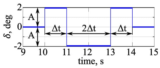
Figure 3.
Multi-step input scheme.
Switching time is the base time period at which the input holds its amplitude. It can be easily defined by using Marchand method [34]. In the method, Bode plots that present contributions of aerodynamic derivatives on the aircraft motion are created. The plots are used to select excitation frequency for each designed input. A Bode plot presenting the effect of side velocity (), roll rate (), and yaw rate () aerodynamic coefficients on yawing moment N when the motion is caused by right elevator deflection is presented in Figure 4. The inertia term is also shown in the plot.
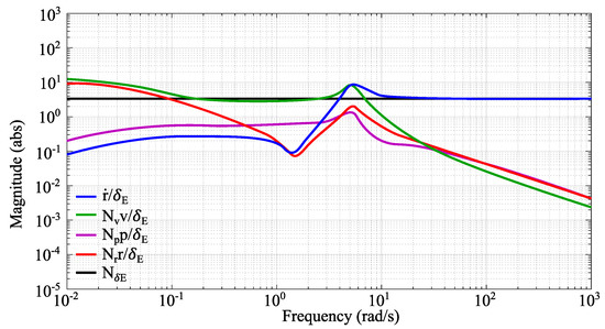
Figure 4.
Bode plot for yawing moment derivatives due to elevator deflection.
On the basis of Bode magnitude plots, it is possible to select frequency ranges in which aerodynamic derivatives can be estimated. A rule of thumb is that a parameter can be estimated when the magnitude of its term is at least 10% of the largest term magnitude. Additionally, if the inertia term magnitude is below the 10% criteria, it means that, at this frequency, the aerodynamic parameters can be identified as a ratio between themselves [22,35,36].
From Figure 4, it can be seen that, for frequencies lower than 0.2rad/s, the greatest contribution to yawing moment due to right elevator deflection is related to component. In the range <0.2; 1.8 > rad/s the greatest influence comes from the contribution. In (1.8; 5 > rad/s) frequency range, the again has the greatest contribution. Above 5 rad/s the greatest magnitude is observed for the inertia term. According to the given rule of thumb (10% of the largest term magnitude), this means that derivative can be accurately estimated if the excitation frequency is below 18 rad/s, can be accurately estimated in the frequency range <0.07; 6.8 > rad/s, when the frequency is below 0.8 or in <2.6; 12 > rad/s frequency range and for all frequencies. However, the mentioned derivatives can be directly estimated (not as a ratio) when the elevator input is used if the frequency is above 2.05 rad/s, because the inertia term contribution will be large enough.
When frequencies are selected for each input, the switching times are evaluated. For a doublet signal, this is equal to half of the oscillation period, as the linear system representation is usually accurate for flight dynamic purposes and the linear system should respond to the sinusoidal input with scaled and shifted sinusoidal output.
Multi-step inputs are usually applied to deflect a single flight control (or their pair) at a time, as, in this case, no additional dynamics (coming from another excitation) is observed in the data and thus does not lower the accuracy of parameter estimation. However, it is possible to design multi-step inputs, in which multiple flight controls are simultaneously deflected without lowering the accuracy e.g., to shorten the experiment time and reduce cost [26]. In the study, the simultaneous multi-axis input was required to include how a single flight control deflection influence the one from the corresponding pair, as it may happen that the excitations will be different because of the necessity to reconfigure the aircraft. In other words, right and left aileron, right and left elevator part, and right and left flap were independently deflected and it was possible that left and right flight control were deflected at a different angle at the same time.
Fisher Information matrix F [22] was used to find the set of simultaneous deflections that does not lower the information content stored in the data due to responses from one input affecting another:
where is the likelihood function, z are the measurements and are the system parameters to be estimated.
Multivariate normal distribution was selected to define the likelihood function, which allows to approximate Fisher Information matrix:
where y are the model outputs, u is the designed input, is the time at k-th point, and and R is the measurement noise covariance matrix.
As the Fisher Information matrix columns are related to the model outputs and rows to the estimated system parameters its determinant maximization aims at maximizing diverse information that will be provided by the designed input:
This is known as the D-optimality, which is the most frequently used criterion in optimal experiment design [37]. The criterion is invariant to system scaling and it helps to minimize redundancy in the data. It would be possible to use other experiment design optimality criterion e.g., E-optimality, which maximizes the minimum eigenvalue, or V-optimality, which minimizes the average prediction variance. However it was already shown that, if another criterion would be used, the results would be also suitable in terms of D-optimality [26].
The optimal excitations were designed for three cases—in each, only flight controls that are usually deflected in pairs were allowed to be excited. Each input could accept one of three states (negative amplitude, zero value, positive amplitude) in each of ten intervals. The design variables were the input states in each interval. The intervals began after each other and their length was equal to the switching time that resulted from the Bode plot. The rudder was consisting of only one surface, thus it was not required to use D-optimality criterion to design input signal for this flight control. To excite rudder, a doublet signal was selected and its switching time resulted from the Bode plots.
Figure 5 presents the designed multi-step inputs for flight controls that can act in pairs. The rudder was deflected with a doublet for which the switching time was 0.74 s and the amplitude was 3 deg. Each flight control deflection was proceeded by a 5 s trimmed flight in order to allow for static components estimation.
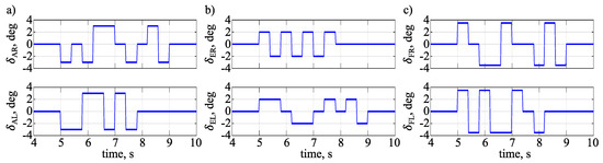
Figure 5.
Multi-step exciattions for: (a) ailerons, (b) elevator parts, (c) flaps.
To find the solution (shown in Figure 5) for ailerons, elevator parts and flaps (signal values for each interval) a genetic algorithm was used due to the large search space size ( possible solutions) and multiple local minima. The algorithm scheme is presented in Figure 6.
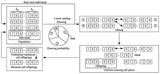
Figure 6.
Multi-step signals optimization scheme.
As said, input values in each interval (negative amplitude, zero, and positive amplitude) for left and right flight control were selected as the design variables. Sets consisting of design variables for left and right flight control were coded by using a ternary representation (0 = negative amplitude, 1 = zero value, 2 = positive amplitude) and each set formed an individual. The individuals (that were found after optimization) are shown in Figure 5 and referred here for better understanding. The input that is presented in Figure 5a) corresponds to the individual 01022101200022020111. The first 10 elements of this string (0102210120) describe right aileron deflection and the remaining 10 elements (0022020111) the left aileron deflection. The elements represent signal values during each interval, which means that the right aileron input starts with negative deflection (0), then a zero value is held (1), which is followed by a negative deflection (0). The length of those deflections is equal to the switching time. Subsequently, the deflection is positive and lasts two switching times (22). After that a zero value is hold (1), which is followed by a negative deflection (0), zero value (1), positive deflection (2), and negative deflection (0). The left aileron deflection starts with negative deflection lasting two switching times (00), which is followed by a positive deflection of the same duration (22). Subsequently, a negative (0), positive (2), and negative (0) deflections are applied, and duration for each of them is equal to the switching time. The left aileron excitation finishes with a zero value that lasts for three switching times (111). The elevator parts and flaps are coded analogously. The input that is presented in Figure 5b) corresponds to the individual 20202020002210012120 and in Figure 5c) to 21002110202020021011. In both cases, the first 10 elements of each string describe the right flight control and the last 10 elements the left flight control.
Subsequently, selected individuals were used to create new solutions. The common way for the selection stage is to draw the individuals according to their cost function, as this allows for putting more emphasis on better solutions, while still keeping diversity in the population. In the study, the cost function for each individual was evaluated and the individuals were sorted with respect to their cost function. Subsequently, a probability was assigned according to their position in the set and the individuals were drawn. This strategy allows for eliminating the quick loss of diversity in the population if an individual that has much better cost function than others is created (in case it represents a local minimum) and it is known as linear drawing.
In Figure 6, the drawing process is shown in the pie chart for four individuals. The ranks present positions of the individuals in the sorted set - the individual with the lowest cost function has rank 1 and the ranks ascend when the cost function increases. The area of each slice represents the probability of each individual to be drawn. This probability is the greatest for the best individual (lowest cost function) and lowest for the worst one (highest cost function).
The drawing probability of the i-th ranked individual was:
where the minimum and maximum drawing probabilities are:
and M is the number of individuals.
After drawing an individual, it was mated (paired) with the next drawn individual. The individuals were independently mated on their position in the set and the only restriction in the drawing process was that the individual could not be mated with itself. If a situation like this occurred, the drawing process of the mated individual was repeated. It also means that it was possible to draw the same individual more than once.
In each pair, uniform crossover was performed in order to exchange the information between the individuals. This means that, for each pair, a random mask that was filled with 0 and 1 was drawn. The length of the mask was the same as of the individual. If 0 was drawn in the mask field, the corresponding design variable value was taken from the first individual to form the first offspring. If 1 was drawn, then the corresponding design variable value was taken from the second individual to form the second offspring. The rest of the design variables formed the second offspring.
To increase the diversity in the population a mutation operator was introduced—the design variables were allowed to change their value with 5% probability. The new value of the design variable was drawn from the remaining set. The probability that the design variable will change was evaluated for each individual. After the mutation operator was applied to all offspring a new population was created and the process was repeated. In the new population, the best individual from the previous population was additionally stored. The optimization was stopped if after 10 iterations no change in the cost function of the best individual was observed. This value was based on the experience and allowed to terminate the optimization faster than when a total number of iterations is used as a stop criterion. The initial population was drawn and counted 300 individuals. During the studies, it was found that, when a smaller population was used (250 individuals), more iterations were required to find the solution, so the computational time was comparable. Moreover it was also observed, that it was not always possible to find a solution with comparable cost function, as there was not enough diversity in the population. When more individuals (350) were used the solution was obtained with less iterations but as more evaluations were performed the optimization was slightly longer. If a greater population was used (400, 450, or 500 individuals) more iterations were required due to greater population diversity and the obtained solution was not better than when population counted 300 or 350 individuals. 5% changes in mutation probability (in order to increase diversity) did not allow to solve described issues for 250 individuals. The same was observed when the mutation probability was lowered by 5% (i.e., no mutation was applied) for populations with 400 and more individuals. When a 10% mutation probability was used for 300 and 350 individuals the number of iterations increased due to greater diversity in the population.
4. Multisine Inputs
The multi-step inputs design was assessed by selecting other type of system identification excitations that allows for simultaneous flight control deflections and comparing the accuracy of the estimates [27]. This approach makes it possible to observe unadded object dynamics and find or discard dependence between stability and control coefficients. The multisine inputs were chosen for that purpose and SIDPAC package [27] was used to design them. The package is a set of Matlab scripts that allow for performing aircraft system identification tasks, including: data compatibility check, filtering, parameter estimation, and validation. The outcomes obtained with SIDPAC package are in good agreement with those from other available tools designed for aircraft system identification e.g., Matlab scripts form [22] or CIFER software [38].
The multisine input consists of summed sinusoidal components. If two excitations only consist of various sinusoidal components that are harmonically related, then their energy spectrum is discrete and composed of various spectral lines. This means that the response of the system, which is caused by a particular excitation can be observed with the same information content, regardless of other excitations present in the experiment. In other words, each harmonic must be assigned to only one flight control to assure excitation by simultaneous multisine signals that can provide high accuracy estimates [27]:
where j denotes the input, k is the harmonic component from the set associated to j-th input, , , and are k-th component amplitude, frequency, and phase angle, whilst t stands for time.
Similarly to the multi-step case, four system-identification experiments were designed with multisine inputs: one for simultaneous right and left aileron deflection, one for simultaneous right and left elevator part deflection, one for simultaneous right and left flap deflection, and one for rudder deflection. This means that, in each experiment, maximum two inputs were applied- one for the left system component, one for the right system component.
In each of those experiments harmonics were evenly spaced for both controls–the odd harmonics were assigned for right control and were even assigned for left control. The minimum frequency was 0.1 Hz and the frequency resolution resulted from the excitation time for T = 20 s. The maximum frequency was 2 Hz, as this is the typical limit for flight dynamic purposes if the aircraft is modelled as rigid body. For the rudder, the input excitation time was T = 10 s.
In multi-step design, the same amplitude bounds were applied to each interval. Therefore, in the multisine design, it was decided that harmonic component amplitudes should also have the same value i.e., equal emphasis was put on all harmonic frequencies. The amplitude for each harmonic was [27]:
where is the expected maximum deflection of the flight control and is the number of elements in the set. The expected maximum deflections were 3 deg, 1 deg, 3.75 deg, and 2 deg for ailerons, elevator parts, flaps, and rudder, respectively. If a greater emphasis should be put on certain harmonics, the nonuniform spectrum can be manually designed [21] or optimized [39].
The phase angles were selected to maximize the input efficiency that was expressed by the relative peak factor. The peak factor can be viewed as the ratio between maximum excitation range and the input energy (represented by the signal RMS); thus, this variable was minimized [27]:
The simplex algorithm was used to perform the minimization. The algorithm is implemented in the Matlab fminsearch function, which is used for optimizing nonlinear functions with several variables. To solve the problem, it would be possible to select another direct search method for multidimensional unconstrained minimization. It would also be possible to use a genetic algorithm for multisine optimization, but this would raise the computational time. This was not considered to be necessary, because the aim of the multisine design was to assist the D-optimal inputs and not to compare the design process of both inputs type. It was not possible to use the fminsearch function in the multi-step multi-axis D-optimal design because of the multiple local minima and computational time. After the phase angles were obtained it was required to shift the designed multisine signals, so they start and end with zero value. Similarly, to the multi-step excitation a 5 s of trimmed flight was included before inputs application to allow for static coefficients estimation.
In Figure 7, normalized multisine inputs are presented. Table 2 shows their components. As the difference between ailerons, elevator parts, and flaps inputs was only in expected maximum amplitude their shape and components (besides ) were the same. Therefore, a design in which maximum expected amplitude was equal to 1 is used to present the inputs.
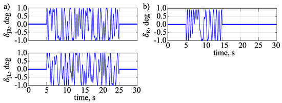
Figure 7.
Multisine excitations for: (a) ailerons, elevator parts and flaps, (b) rudder.
Table 2.
Multisine inputs.
Because the problem is symmetric, it is possible to use left and right control surfaces interchangeably. In the case of nonsymmetric problems (e.g., if the propeller-induced sidewash would be significant), this would not be possible. The same is true also for the presented multi-step inputs. The excitations are applied in pairs (right and left aileron, right and left elevator part, right and left flap) or separately (rudder). If all flight controls would be excited simultaneously, the D-optimal design evaluations would last longer or the cost function would increase. In the case of the multisine signals, this would mean that either the inputs have less frequency components (so estimates accuracy would be reduced) or that higher sampling resolution is required for the gathered data.
5. System Identification
System identification is a method that allows for obtaining accurate aerodynamic coefficients estimates from the conducted experiments if the system is deterministic. This requires accurate measurements of the inputs and outputs with enough information about the object dynamic, as only the phenomena that are present in the data can be identified with low uncertainty. The simultaneous multi-step and multisine inputs that are presented in Section 3 and Section 4 were designed to provide the good information content, as they maximize Fisher Information matrix determinant or minimize relative peak factor.
Among the system identification methods used in flight dynamics, the output error approach is the most used one. This is because its simplicity, ease in results validation, ability to account for measurement noise, and wide range of applicability. The evaluations in the method are usually performed in the time domain; however, a frequency domain approach can be also used e.g., in the case of unstable systems [22]. In the presented study, the time domain approach was used, as the object was dynamically stable and the frequency domain data do not allow directly to include static terms.
The aim of the method is to minimize the difference between the registered outputs and the ones that are obtained from the estimated model for the same inputs. However, it needs to be underlined that the purpose of the estimation is to obtain accurate model parameters estimates (that will produce estimated model outputs that match the measured ones) and not to obtain a good curve match between estimated model outputs and measured outputs. If the model has to many parameters, then it is possible that the estimates will have low accuracy, but at the same time a good match will be observed for all outputs. This may happen, because the optimization algorithm will try to compensate influence of some parameters with others. To solve this issue, the curve matching algorithm cost function is based on maximum likelihood principle that seeks for model parameters that have the greatest probability p of causing measurements z [22]:
When multivariate normal distribution is selected it is preferable to minimize the negative log-likelihood instead of maximizing the conditional probability, as this simplifies the evaluations:
where R is the measurement noise covariance matrix that can be estimated from
Finally the cost function is given as:
To minimize the cost function, the Levenberg–Marquardt algorithm was used, thus the estimates were updated according to the formula:
where F is the Fisher Information Matrix that is given by Equation (13), G is the gradient matrix:
and i denotes iteration number.
The damping factor allows for interpolating between Gauss–Newton and the steepest descent algorithms. The damping factor value in each iteration if found by evaluating cost function without and with damping factor reduction (). First, the cost function from the previous iteration is compared with the current cost function with and without damping factor reduction ( and , respectively). If the current cost function for the reduced damping factor is smaller, then the reduced damping factor is used in the current and consecutive iterations. Or else, the damping factor remains unchanged. If none of those conditions are met, the damping factor is increased ().
In the study, the initial damping factor was = 0.0001 and the reduction factor was = 10. If a relative change in the cost function was below 0.0001, the optimization (i.e., parameter estimation) was finished. Figure 8 shows the scheme of the method.
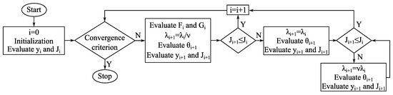
Figure 8.
Optimization algorithm.
6. Results
The nonlinear aircraft model that is presented in Section 2 was excited with the inputs presented in Figure 5. The outputs of the model were registered and corrupted by including measurement noise. Process noise was not included in the data, as the flight tests are usually performed in calm atmosphere. Subsequently, the system was identified using the method that is presented in Section 5 and linear system Equations (3) and (11). The evaluations were performed with sampling time of 0.02 s and Runge–Kutta (4,5) method (ode45 function) was used to integrate the equations. Time sections for all experiments were used in single estimation. The presented approach allowed for observing the best possible accuracy of the estimated aerodynamic coefficients in noise presence when the designed inputs are applied.
Figure 9 presents time histories of the aircraft response to simultaneous multi-step elevator deflection. The blue lines in the plot denote the registered outputs and red lines stand for identified model response. Because, in certain time periods, only one part of the elevator was deflected (or the parts were deflected in opposite directions) side-force, rolling, and yawing moment were also produced. This resulted in lateral-directional motion that accompanied the longitudinal motion. In both cases, a good visual match was observed for all outputs. It can be also seen that the aircraft returns to the equilibrium very quickly, which is desirable as new experiment can be performed and thus flight test campaign time is reduced. Similar conclusions were drawn when the object was excited with the remaining multi-step excitations.
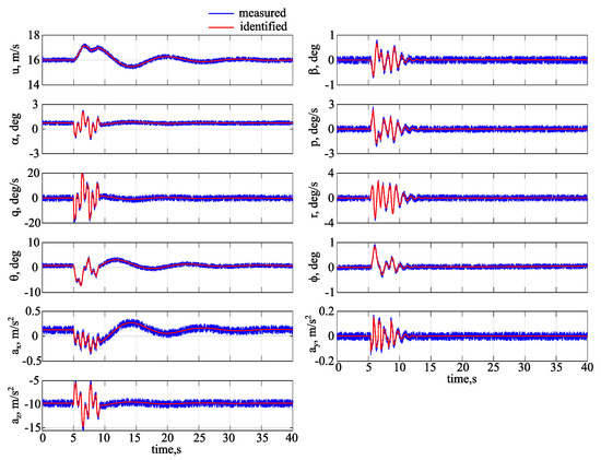
Figure 9.
Time histories for the multi-step elevator input.
As said, in the case of too many model parameters, it may happen that a good visual match is observed, even though the estimates are not accurate. Thus, it is also necessary to investigate model uncertainty, which can be expressed by relative standard deviations of the estimates. This is presented in Table 3 and Table 4. The - symbol in the tables denotes that the aerodynamic coefficient was not was present in the model structure.
Table 3.
Parameters estimated from multi-step experiments.
Table 4.
Relative standard deviations for parameters estimated from multi-step experiments.
It can be seen that the stability and control derivatives were estimated with high accuracy as their relative standard deviations are below 10%, which denotes accurate system identification results [22]. Relative standard deviation for the majority of the aerodynamic coefficients was below 6% and only for three of them (, and ) this value was higher. However, the values of those parameters were very small and, thus, their contribution to the aircraft response can be smaller than for other stability and control derivatives.
The aircraft model was also excited with the multisine inputs that are presented in Section 7. Similarly to the multi-step excitations, the aircraft response was registered, the same measurement noise was added and the system was identified with the same methodology. Time histories of the aircraft response to simultaneous multisine elevator deflection is presented in Figure 10.

Figure 10.
Time histories for the multisine elevator input.
Again, a good match can be seen between the registered outputs and the estimated model response. Similarly to the experiments with multi-step inputs, this was also observed for manoeuvres in which remaining flight controls were excited with multisine signals. It can be also seen that a slightly longer time is required in order to reach the trim point and this results from the longer excitation duration. If a shorter input signal would be used frequency resolution would be lower and some frequencies would be not excited which could lead to lower accuracy of the outcomes.
The estimates and their relative standard deviations are presented in Table 5 and Table 6. The identified parameters values are similar to the ones that were obtained from multi-axis experiments. In general, the accuracy of the estimated aerodynamic derivatives is slightly higher with a mean standard deviation of 2.70%, which, for the outcomes obtained from multi-axis maneuvres, was 4.16%. Relative standard deviations are below 4% for all except three model parameters. Those are the same as for multi-step case (, and ) and, again, this can be associated with their small value that may indicate small contribution to the total aircraft response.
Table 5.
Parameters estimated from multisine experiments.
Table 6.
Relative standard deviations for parameters estimated from multisine experiments.
Similar results were obtained when Ordinary Least Squares were used to estimate the parameters. The solution was obtained by using the equation [22]:
where X and Y are the independent and dependent variables, respectively. State and control vectors were used as the independent variables and the time derivatives of the state vector as the dependent variables. Central differences were used to compute the derivatives. The equations describing the system were given by (3) and solved independently. It was observed that the estimates were of high accuracy, but the mean standard deviation increased to 6.78% for multi-step design and to 5.61% when multisines were used. Again, the lowest accuracy was observed for , , and coefficients. Those outcomes show that designed inputs allow for obtaining accurate estimates, even if different system identification method is used.
7. Conclusions
In this paper, a design of multi-axis multi-step system identification experiment for reconfigurable fixed-wing unmanned aerial vehicle was presented. It was shown that the experiment allows for obtaining very accurate estimates of stability and control coefficients in noise presence. Moreover, the aircraft quickly returns to the trim point, which, together with simultaneous flight, controls deflections benefits in limited flight test campaign time.
For the same object, a system identification experiment with simultaneous multisine excitations was designed. For the same object, a system identification experiment with simultaneous multisine excitations was designed. In this case, the aerodynamic parameters were estimated with slightly lower standard deviations, which denotes higher accuracy (the mean standard deviation was lower by 1.46%). The time required to return to the trim point was slightly greater (10 s), as the excitation had to last longer.
Presented inputs were used in the flight campaign. Gathered flight data allowed for obtaining a mathematical model of the object, which was used later to design the reconfiguration system that is presented in [14]. In future works, it was planned to improve the multi-step optimization e.g., by using swarm particle optimization. It should be also investigated whether it is possible to increase the accuracy of the estimates by including more information in the data through relating excitations frequencies with time at which their appear. The discrete wavelet transform is to be used for that purpose.
Funding
This research was funded by the National Centre for Research and Development (NCBiR) under project “Methodology of aircraft control system synthesis under high risk circumstances”, NCBiR, PBS2/B6/19/2013.
Acknowledgments
The author would like to thank German Aerospace Center (DLR) for the support he received during his stay in the Institute of Flight Systems (FT) in Braunschweig and the guidance he received after the stay had finished.
Conflicts of Interest
The author declare no conflict of interest. The funders had no role in the design of the study; in the collection, analyses, or interpretation of data; in the writing of the manuscript, or in the decision to publish the results.
References
- Takahashi, T.T.; Perez, R.E. The Effect of Manufacturing Variation on Aerodynamic Performance and Flight Safety. In AIAA AVIATION 2020 FORUM; AIAA: Dallas, TX, USA, 2020; p. 2649. [Google Scholar] [CrossRef]
- Uehara, A.F.; Niedermeier, D. Influence of coupled sidesticks on the pilot monitoring’s awareness during flare. In AIAA Modeling and Simulation Technologies Conference; AIAA: Dallas, TX, USA, 2015; p. 2338. [Google Scholar] [CrossRef]
- Khan, W.; Ansell, D.; Kuru, K.; Bilal, M. Flight Guardian: Autonomous Flight Safety Improvement by Monitoring Aircraft Cockpit Instruments. J. Aerosp. Inf. Syst. 2018, 15. [Google Scholar] [CrossRef]
- Quaranta, G.; Tamer, A.; Muscarello, V.; Masarati, P.; Gennaretti, M.; Serafini, J.; Colella, M.M. Rotorcraft aeroelastic stability using robust analysis. CEAS Aeronaut. J. 2014, 5, 29–39. [Google Scholar] [CrossRef]
- Hess, R.A. Modeling Human Pilot Adaptation to Flight Control Anomalies and Changing Task Demands. J. Guid. Control. Dyn. 2015, 39. [Google Scholar] [CrossRef]
- Kopyt, A.; Topczewski, S.; Zugaj, M.; Bibik, P. An automatic system for a helicopter autopilot performance evaluation. Aircr. Eng. Aerosp. Technol. 2019, 91, 880–885. [Google Scholar] [CrossRef]
- Tamer, A.; Muscarello, V.; Quaranta, G.; Masarati, P. Cabin Layout Optimization for Vibration Hazard Reduction in Helicopter Emergency Medical Service. Aerospace 2020, 7, 59. [Google Scholar] [CrossRef]
- Deiler, C.; Fezans, N. VIRTTAC - A Family of Virtual Test Aircraft for Use in Flight Mechanics and GNC Benchmarks. In AIAA Scitech 2019 Forum; AIAA: San Diego, CA, USA, 2019. [Google Scholar] [CrossRef]
- Humphreys-Jennings, C.; Lappas, I.; Sovar, D.M. Conceptual Design, Flying, and Handling Qualities Assessment of a Blended Wing Body (BWB) Aircraft by Using an Engineering Flight Simulator. Aerospace 2020, 7, 51. [Google Scholar] [CrossRef]
- Topczewski, S.; Narkiewicz, J.; Bibik, P. Helicopter Control During Landing on a Moving Confined Platform. IEEE Access 2020, 107315–107325. [Google Scholar] [CrossRef]
- Crider, D. Control System Failure Simulation for Accident Investigation. In AIAA Modeling and Simulation Technologies Conference and Exhibit; AIAA: San Francisco, CA, USA, 2005; p. 6113. [Google Scholar] [CrossRef]
- Steinberg, M. A historical overview of research in reconfigurable flight control. Proc. Inst. Mech. Eng. Part J. Aerosp. Eng. 2005, 219, 263–275. [Google Scholar] [CrossRef]
- Naskar, A.K.; Patra, S.; Sen, S. Reconfigurable Direct Allocation for Multiple Actuator Failures. IEEE Trans. Control. Syst. Technol. 2015, 23, 397–405. [Google Scholar] [CrossRef]
- Kopyt, A.; Żugaj, M. Analysis of Pilot Interaction with the Control Adapting System for UAV. J. Aerosp. Eng. 2020, 33, 04020025. [Google Scholar] [CrossRef]
- Haley, P.; Soloway, D. Aircraft reconfiguration using neural generalized predictive control. In Proceedings of the 2001 American Control Conference, Arlington, VA, USA, 25–27 June 2001; IEEE: Piscataway, NJ, USA, 2001; Volume 4. [Google Scholar] [CrossRef]
- Tingting, Y.; Aijun, L. Flying wing aircraft sliding mode LI adaptive reconfiguration flight control law design. In Proceedings of the 13th International Conference on Control Automation Robotics & Vision (ICARCV), Singapore, 10–12 December 2014; IEEE: Piscataway, NJ, USA, 2014. [Google Scholar] [CrossRef]
- Shan, S.; Hou, Z. Neural Network NARMAX Model Based Unmanned Aircraft Control Surface Reconfiguration. In Proceedings of the 9th International Symposium on Computational Intelligence and Design, Hangzhou, China, 10–11 December 2016; IEEE: Piscataway, NJ, USA, 2016. [Google Scholar] [CrossRef]
- Sun, L.G.; de Visser, C.C.; Chu, Q.P.; Mulder, J.A. Joint Sensor Based Backstepping for Fault-Tolerant Flight Control. J. Guid. Control. Dyn. 2016, 38, 62–75. [Google Scholar] [CrossRef]
- Nasir, A.; Atkins, E.; Kolmanovsky, I. A Mission Based Fault Reconfiguration Framework for Spacecraft Applications. In AIAA Infotech@Aerospace 2012; AIAA: Garden Grove, CA, USA, 2012; p. 2403. [Google Scholar] [CrossRef]
- Usach, H.; Vila, J.A. Reconfigurable Mission Plans for RPAS. Aerosp. Sci. Technol. 2020, 96. [Google Scholar] [CrossRef]
- Morelli, E.A. Flight Test Maneuvers for Efficient Aerodynamic Modeling. J. Aircr. 2012, 49, 1857–1867. [Google Scholar] [CrossRef]
- Jategaonkar, R.V. Flight Vehicle System Identification: A Time Domain Methodology, 2nd ed.; Progress in Astronautics and Aeronautics; AIAA: Reston, VA, USA, 2015. [Google Scholar] [CrossRef]
- Deiler, C. Aerodynamic Modeling, System Identification, and Analysis of Iced Aircraft Configurations. J. Aircr. 2017, 55, 145–161. [Google Scholar] [CrossRef]
- Berger, T.; Tischler, M.B.; Knapp, M.E.; Lopez, M.J.S. Identification of Multi-Input Systems in the Presence of Highly-Correlated Inputs. J. Guid. Control. Dyn. 2018, 41, 2247–2257. [Google Scholar] [CrossRef]
- Lichota, P.; Szulczyk, J.; Tischler, M.B.; Berger, T. Frequency Responses Identification from Multi-Axis Maneuver with Simultaneous Multisine Inputs. J. Guid. Control. Dyn. 2019, 42, 2550–2556. [Google Scholar] [CrossRef]
- Lichota, P.; Sibilski, K.; Ohme, P. D-Optimal Simultaneous Multistep Excitations for Aircraft Parameter Estimation. J. Aircr. 2017, 54, 747–758. [Google Scholar] [CrossRef]
- Morelli, E.A. Multiple Input Design for Real-time Parameter Estimation in the Frequency Domain. In Proceedings of the 13th IFAC Conference on System Identification, Rotterdam, The Netherlands, 27 August 2003; IFAC: Rotterdam, The Netherlands, 2003. [Google Scholar] [CrossRef]
- MULTIPLEX Modellsport GmbH. Multiplex Cularis Manual; MULTIPLEX Modellsport GmbH: Bretten, Germany, 2007. [Google Scholar]
- Cook, M.V. Flight Dynamics Principles, 3rd ed.; Elsevier: Amsterdam, The Netherlands, 2013. [Google Scholar] [CrossRef]
- Anonymous. Flying Qualities of Piloted Aircraft; Technical Report MIL-STD-1797A; Department of Defense: Arlington, VA, USA, 1997. [Google Scholar]
- Anonymous. Aeronautical Design Standard, Handling Qualities Requirements for Military Rotorcraft; Technical Report ADS-33E-PRF; U.S. Army Aviation and Missile Command: Redstone Arsenal, AL, USA, 2000. [Google Scholar]
- Wells, W.; Ramachandran, S. Multiple Control Input Design for Identification of Light Aircraft. IEEE Trans. Autom. Control 1977, 22, 985–987. [Google Scholar] [CrossRef]
- Seren, C.; Bommier, F.; Verdier, L.; Bucharles, A.; Alazard, D. Optimal Experiment and Input Design for Flight Test Protocol Optimization. In AIAA Atmospheric Flight Mechanics Conference and Exhibit; AIAA: Keystone, CO, USA, 2006; p. 6280. [Google Scholar] [CrossRef]
- Marchand, M. Untersuchung der Bestimmbarkeit von Fleugzeugderivativen aus Flugversuchen; Technical Report DFVLR-IB 154-74/32; DLR: Braunschweig, Germany, 1974. [Google Scholar]
- Plaetschke, E.; Schulz, G. Practical Input Signal Design; Technical Report LS-104; AGARD: Neuilly sur Seine, France, 1979. [Google Scholar]
- Carnduff, S. System Identification of Unmanned Aerial Vehicles. Ph.D. Thesis, Cranfield University, Cranfield, UK, 2008. [Google Scholar]
- Goodwin, G.C.; Payne, R.L. Dynamic System Identification: Experiment Design and Data Analysis; Mathematics in Science and Engineering, Academic Press: New York, NY, USA, 1977. [Google Scholar]
- Tischler, M.B.; Remple, R.K. Aircraft and Rotorcraft System Identification, 2nd ed.; AIAA Education Series; AIAA: Reston, VA, USA, 2012. [Google Scholar] [CrossRef]
- Lichota, P.; Szulczyk, J.; Noreña, D.A.; Monsalve, F.A.V. Power Spectrum Optimization in the Design of Multisine Manoeuvre for Identification Purposes. J. Theor. Appl. Mech. 2017, 55, 1193–1203. [Google Scholar] [CrossRef]
© 2020 by the author. Licensee MDPI, Basel, Switzerland. This article is an open access article distributed under the terms and conditions of the Creative Commons Attribution (CC BY) license (http://creativecommons.org/licenses/by/4.0/).