Static Aeroelastic Beam Model Development for Folding Winglet Design

Abstract

Wing shape adaptability during flight is the next step towards the greening of aviation. The shape of the wing is typically designed for one cruise point or a weighted average of several cruise points. However, a wing is subjected to a variety of flight conditions, which results in the aircraft flying sub-optimally during a portion of the flight. Shape adaptability can be achieved by tuning the shape of the winglet during flight. The design challenge is to combine a winglet structure that is able to allow the required adaptable shape while preserving the structural integrity to carry the aerodynamic loads. The shape changing actuators must work against the structural strains and the aerodynamic loads. Analyzing the full model in the preliminary design phase is computationally expensive; therefore, it is necessary to develop a model. The goal of this paper is to derive an aeroelastic model for a wing and winglet in order to reduce the computational cost and complexity of the system in designing a folding winglet. In this paper, the static aeroelastic analysis is performed for a regional aircraft wing at sea level and service ceiling conditions with three degree and eight degree angle of attack. MSC Nastran Aeroelastic tool is used to develop a Finite Element Model (FEM), i.e., beam model and the aerodynamic loads are calculated based on a doublet lattice panel method (DLM).

1. Introduction

Aeroelasticity is a discipline that studies the phenomena that involve the interaction between aerodynamic forces and elastic forces. This study is crucial due to two main reasons. First, the interaction can lead to static or dynamic instabilities that can result in failure of the structure. Secondly, the loads calculated using aeroelastic simulations are significantly different for flexible structures as compared to decoupled structural and aerodynamic simulations. This has significant influence on the design and weight of the structure, and its aerodynamic performance. Aeroelasticity is divided in to two main groups as Static and Dynamic aeroelasticity. Static aeroelasticity is the study of the deflection of flexible aircraft structures under aerodynamic loads, where the forces and motions are considered to be independent of time. Dynamic aeroelasticity studies the interactions among aerodynamic, elastic, and inertial forces. Examples of dynamic aeroelastic phenomena are Flutter, Buffeting, and Transonic aeroelasticity. General Form of the Aeroelastic Equations is

$$A\ddot{q}+(\rho VB+D)\dot{q}+(\rho V^{2}C+E)q=0$$

(1)

where q is the generalized coordinates, A is the structural inertia, B is aerodynamic damping, C is aerodynamic stiffness, D is structural damping, and E is the structural stiffness matrices. Equation (1) is one of the most important equations and it describes the fundamental interaction between the flexible structure and the aerodynamic forces [1].

Morphing is a capability to provide superior performance while in flight by tailoring the vehicle’s state to adapt to the external operating environment and multivariable mission roles. Morphing aircraft are multi-role aircraft that change their external shape in both small-scale and large-scale substantially to adapt to a changing mission environment during flight. Bowman et al. identified two distinct classes of morphing: Morphing for Mission Adaptation, and Morphing for Control. Morphing for Mission Adaptation is a large-scale, relatively slow, in-flight shape change to enable a single vehicle to perform multiple diverse mission profiles. On the contrary, Morphing for Control is often a small-scale or component level in-flight physical or virtual shape change, being used to achieve multiple control objectives, such as noise suppression, flutter suppression, load alleviation, and active separation control [2].

2. Morphing Winglet with Aerodynamic Actuation

Morphing wings have large potential to improve the overall aircraft performances, by dynamically optimizing the shape to various flight conditions. The morphing winglet is a promising solution among the morphing technologies due to its small size and large effect on the aerodynamics. In this paper, the morphing winglet has to change its cant angle, and its stiffness has to be large enough to carry loads. While increasing the total stiffness, the allocation of the stiffness can be unsymmetrical, introducing deformation under a linear actuation force. A simplified beam model is developed to estimate the induced deformation. The deformation is also visualized using finite element analysis. To demonstrate the application of the morphing structure, the baseline wing design of a regional twin turboprop airliner ATR 72 is used [3,4].

There are different suggested concepts to actuate the folding winglet mechanism. Some which were addressed in previous works are: hinge line actuator, system of pulley gears, and a worm gear system. Each of these systems have their own advantages and disadvantages. The advantage of the hinge line actuator is that the direct connection between the actuators and the hinge line mitigates additional transmission losses, making the system more efficient. The disadvantage is the loss in the winglet area due to the mounting position of the actuator. An additional disadvantage due to its location is the actuator mass will maximize the root bending moment and is susceptible to damage should the aircraft have a tip strike upon landing or take off. The advantage of the system of pulley gears is ability to bring actuation component inboard by maximizing the winglet surface area. The advantage of a worm gear system is the power off locking capability. Power is not required for the system when remaining in one position, because the wheel cannot rotate unless the screw is actively driven. The worm drive acts to gear the system, enabling larger torques to be developed. This could be advantageous by allowing a less powerful (smaller) actuator to be used, but it will also make the system slower. Figure 1 and Figure 2 graphically represent the proposed concepts [5,6].

In this project, the topic of investigation is applying a secondary shape changing mechanism that will alter the aerodynamic loads before the folding angle shape change. The alteration of loads should be such that the aerodynamic loads themselves change the cant angle of the winglet. The envisioned shape changing mechanism to achieve this is a twisting winglet. In summary, the change in folding angle of the winglet will be achieved by first twisting the winglet, changing the local aerodynamic loads such that they will work with the folding angle change rather than work against it. The advantage of aerodynamic actuation is a reduction in the actuator cost and weight. The design challenge is to combine a winglet structure that is able to allow the required adaptable shape while preserving the structural integrity to carry the aerodynamic loads. The shape-changing actuators have to work against the structural strains and the aerodynamic loads. This contradictory requirement often leads to rather heavy actuators that are needed to effectuate the desired shape change [7].

3. Materials and Methods

The flow chart in Figure 3 shows the approach taken while performing the modeling and analysis of the problem. The first step is to import the wing and perform clean up and prepare it to the structural modelling. In the structural model, the geometry is divided into elements and the material properties are distributed. Later, the lifting surface definition and panel box divisions are performed in the aerodynamic modeling. Once we have the structural and aerodynamic grids, the interpolation is carried out using theory of infinite beam splines. Finally the analysis is performed and the desired results are viewed at the post processing. In Figure 4, a three-dimensional (3D) base wing CAD model and two-dimensional (2D) wing with winglet is represented. All CAD models are done on SolidWorks.

4. Structural Model

The structure is modelled as a beam element. Generally, beam models are developed based on various assumptions that lead to different level of accuracy. Several beam theories have been developed; the Euler–Bernoulli beam theory, first described by Euler and Bernoulli, is one of the simplest and most useful theories. A fundamental assumption of this theory is that the cross-section of the beam is infinitely rigid in its own plane, i.e., no deformations occur in the plane of the cross-section. Consequently, the in-plane displacement field can be simply represented by two rigid body translations and one rigid body rotation. This fundamental assumption deals only with in-plane displacements of the cross-section. Two additional assumptions deal with the out-of-plane displacements of the section: during deformation, the cross-section is assumed to remain plane and normal to the deformed axis of the beam. While these assumptions work fine for thin beams under static loading, for thicker beams and higher frequencies they are an oversimplification. In order to overcome these restrictions, the more complex Timoshenko Beam theory was formulated in 1921 and extends the Euler-Bernoulli theory by taking shear deformation and the rotary inertia into account [8].

4.1. Beam Section

There are different techniques for reducing detailed finite elements models, such as static condensation of mass and stiffness matrices, stick models, etc. The stick models are simplified beam finite element models commonly used in civil aircraft design and multidisciplinary design optimization (MDO). The accuracy of the stiffness characteristics in its model highly affects the accurate prediction of bending and twisting deformations of the aircraft structure in flight.

The stick model is usually generated by extracting the stiffness properties of the main structure and applying it to a set of beam elements extending along the structure’s elastic axis. This work exposes a methodology to extract section properties for beam elements while using the Femap surface property generator. Femap calculates all the surface properties by selecting the desired surface. Subsequently, those properties are transferred into the beam element. There are different levels of structural modelling, 3D finite element model is always prepared once the aircraft’s layout and structural details are obtained. The three dimensional finite element model is commonly used in structural design validation and optimization. Imposing a detailed 3D FEM in a multidisciplinary iterative process or in loads analyses is quite expensive. Alternatively, a simplified beam FEM of the wing can be generated and employed in the iterative process and dynamic analyses.

4.1.1. Extracting Beam Sectional Properties

This method extracts the stiffness properties of the beam model from the complete 3D FEM model. The method requires some processing in Femap with Nx Nastran and requires the user to be knowledgeable of the software package. The method assumes that the stiffness extraction process begins by locating the reference coordinate system at the root section of the detailed FEM model; there are no constraints and this coordinate system could be located anywhere in the section. To make the description of the procedure easier, the coordinate reference system is the same for all the parameters, defined as the one of Figure 5; the general axis of the beam model is the z-axis [9].

$$\left\{F\right\}=\left[K\right]\left\{u\right\}\to {\left[K\right]}^{-1}\left\{F\right\}=\left\{u\right\}\to \left[FF\right]\left\{F\right\}=\left\{u\right\}$$

(2)

where F is the vector of forces and moments, u is the displacements vector, [K] is the stiffness matrix, and [FF] is the flexibility matrix. The wing and winglet geometric properties and beam characteristics are mentioned in

Table 1. Base Wing Beam Characteristics.

	Geometrical Properties
Area	27.675	m${}^2$
$I_1$	410.2292	m${}^4$
$I_2$	10.38966	m${}^4$
$I_{1}2$	0	m${}^4$
J	36.56909	m${}^4$
$YShearArea$	23.45501	m${}^2$
$ZShearArea$	20.07553	m${}^2$

and

Table 2. Winglet Beam Characteristics.

	Geometrical Properties
Area	1.6875	m${}^2$
$I_1$	0.304687	m${}^4$
$I_2$	0.197754	m${}^4$
$I_{1}2$	0	m${}^4$
J	0.374914	m${}^4$
$YShearArea$	1.398002	m${}^2$
$ZShearArea$	1.354963	m${}^2$

. Aluminum 2024 was the material of choice and the material properties are listed in

Table 3. Material Properties.

	Aluminum 2024 Annealed Wrought
$YoungsModulus,E$	7.3084 × 10${}^{10}$	N/m${}^2$
$ShearModulus,G$	2.79 × 10${}^{10}$	N/m${}^2$
$Poisso{n}^{\prime }sRatio,\nu$	0.33
$ExpansionCoefficient$, $\alpha$	0	m/m/${}^{\circ }$C
$Conductivity,k$	188.18	Watt/m ${}^{\circ }$C
$SpecificHeat,C_p$	921	J/Kg ${}^{\circ }$C
$MassDensity$	2767.99	Kg/m${}^3$
$ReferenceTemp$	23.9	${}^{\circ }$C

.

4.1.2. CBEAM Element

CBEAM entry defines a beam element in Nastran and its properties are defined with a PBEAM, PBCOMP, or PBEAML entry. The beam element includes extension, torsion, bending in two perpendicular planes, and the associated shear.

Tensile stresses are given a positive sign and compressive stresses a negative sign. Only the longitudinal stresses are available as complex stresses. The stress recovery coefficients on the PBEAM entry are used to locate points on the cross section for stress recovery. Because there is no torsional stress recovery for the CBEAM element, the margin-of-safety computation does not include the torsional stress [10].

The blue curve in Figure 6 shows the beam element model of the wing and winglet.

5. Aerodynamic Model

Doublet-Lattice Subsonic Lifting Surface Theory (DLM)

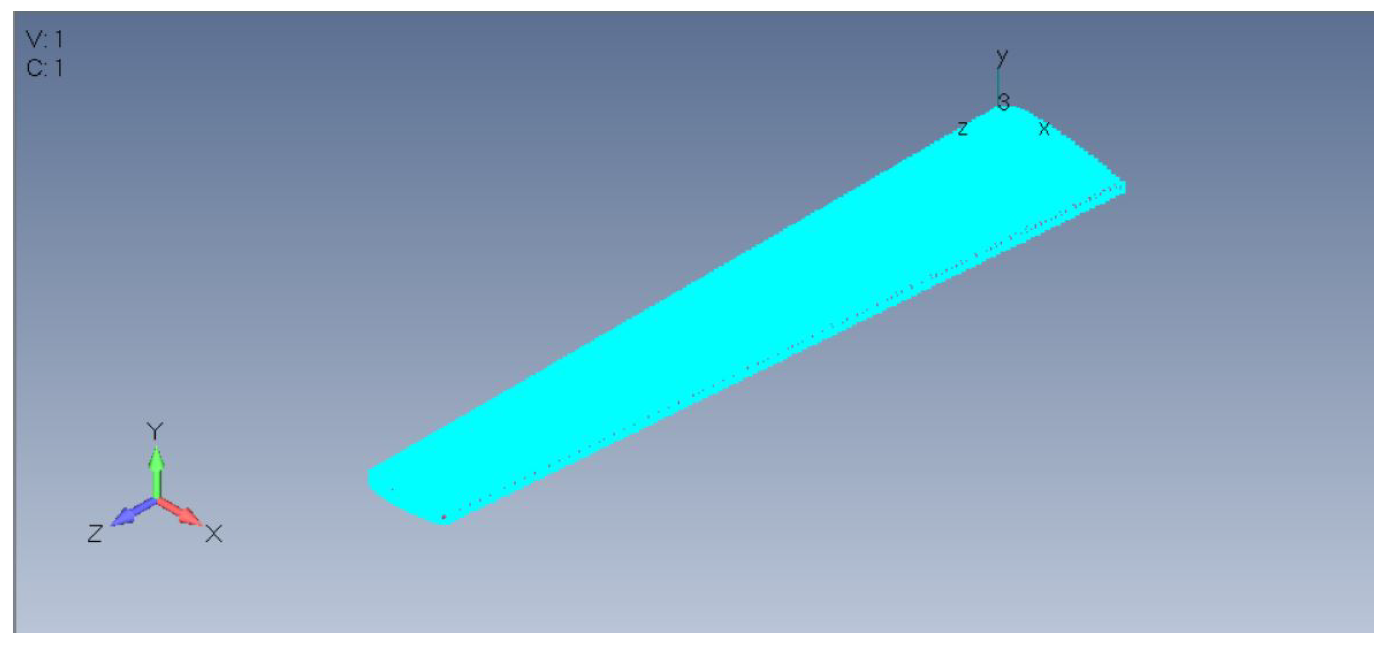
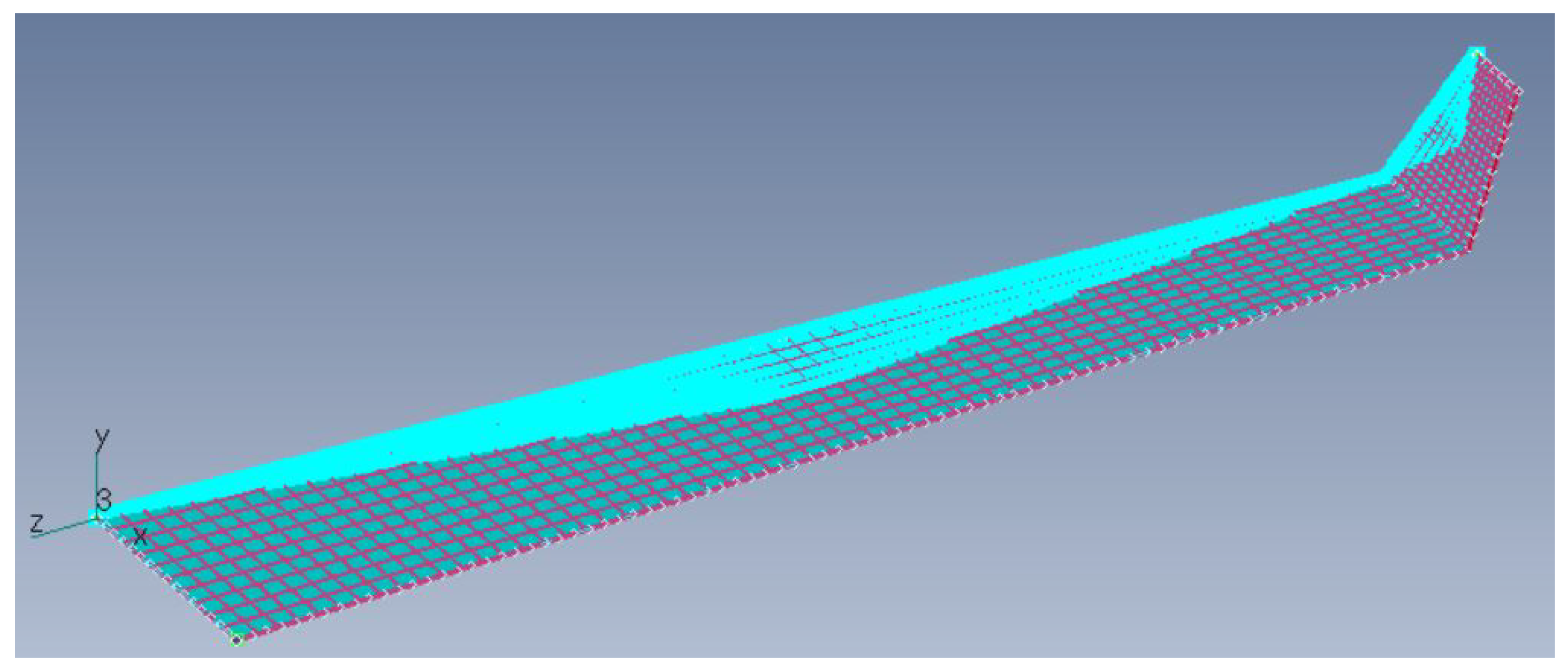
The DLM is an aerodynamic finite element method for modelling oscillating lifting surfaces that reduces to the Vortex-Lattice Method at zero reduced frequency. Each of the interfering surfaces (or panels) is divided into small trapezoidal lifting elements (“boxes”), such that the boxes are arranged in strips parallel to the free stream with surface edges, fold lines, and hinge lines lying on box boundaries. Uniform concentration of the unknown lifting pressures across the one-quarter chord line of each box is assumed. On the three-quarter chord line of the box there is one control point per box centered span-wise and the surface normal wash boundary condition is satisfied at each of these points. The number of finite elements (boxes) required for accurate results depend on different parameters, such as the aspect ratio and reduced frequency. At high reduced frequency, the chord-wise dimension of the boxes must be small. However, an approximation in the method that the variation of the numerator of the incremental oscillatory kernel function is parabolic across the span of the box bound vortex, restricts the box aspect ratio to approximately 3. If a higher order approximation is used for the span-wise variation of the numerator of the incremental oscillatory kernel, the limitation on box aspect ratio can be relaxed and the number of span-wise divisions required in high-frequency analyses will be reduced significantly, leading to a reduction in the total number of boxes. The DLM is a FEM for the solution of the oscillatory subsonic pressure-normal-wash integral equation for multiple interfering surfaces.

$$w(x,s)=(1/8\pi )\sum _{n=1}^N(\int {\int }_{s_n}K(x,\xi ,s,\sigma )p(\xi ,\sigma )d\xi d\sigma$$

(3)

where w is the complex amplitude of the dimensionless normal wash, p is the complex amplitude of the lifting pressure coefficient, (x,s) is the orthogonal coordinates on the nth surface S, such that the undisturbed stream is parallel to the x-axis, and K is the complex acceleration potential kernel for oscillatory subsonic flow. The original DLM algorithm was presented at the same time (1968) as the Lifting Line Element Method (LLEM) of Stark®. Although numerous comparisons@ with experiments were shown at the time, the complete details of the LLEM were never published. A refinement to the expressions for the kernel given by Rodemich® and Landahl was presented by Rodden, Giesing, and Kalman in the form

$$K=(K_1,T_1,/r^2+K_2{T}_2^{*}/r^4)exp(-i\omega \overline{x}/U)$$

(4)

in order to analyze the non-planar interference correctly. $K_1$, and $K_2$, are the planar and non-planar parts of the kernel numerator, respectively. Here, $\omega$ is the frequency, $x_0$ is the distance between the sending and receiving points parallel to the freestream, and U is the velocity of the freestream,

$$T_1=cos({\gamma }_r-{\gamma }_s)$$

(5)

$$T_2^{*}=(z_{0}cos{\gamma }_r-y_{0}sin{\gamma }_r)(z_{0}cos{\gamma }_s-y_{0}sin{\gamma }_s)$$

(6)

$$r^2=z_0^2+y_0^2$$

(7)

where $y_0$ and $z_0$ are the Cartesian distances between sending and receiving points perpendicular to the freestream, and ${\gamma }_r$ and ${\gamma }_s$ are the dihedral angles at the receiving and sending points, respectively. The description of $K_1$ and $K_2$ as the planar and non-planar parts of the kernel numerator is a convenience, because both are obviously non-planar in general. The refinement in the equation was found necessary so that the DLM could predict the interference between a nearly planar wing and horizontal tail, The refinement retained the original primary approximation, i.e., that the incremental oscillatory normal wash factors are obtained by integrating the difference between the oscillatory and steady kernels over the length of the bound vortex assuming a quadratic (parabolic) variation in the numerator of the difference. The total normal-wash factor is then the sum of the incremental oscillatory normal-wash factor and the steady normal-wash factor obtained from the expressions for a horseshoe vortex, e.g., the Vortex—Lattice Method (VLM) of Hedman. In this way, the DLM converges to the VLM at zero reduced frequency, and the error in the parabolic approximation of the kernel numerator difference is small at low reduced frequencies and increases with the reduced frequency [11,12].

The Doublet–Lattice method (DLM) can be used for interfering lifting surfaces in subsonic flow. The following general remarks summarize the essential features of the method.

• The theoretical basis of the DLM is linearized aerodynamic potential theory.
• The undisturbed flow is uniform and is either steady or varying (gusting) harmonically.
• All lifting surfaces are assumed to lie nearly parallel to the flow.

The panel divisions for the wing are presented in the Figure 7 and Figure 8.

6. Interconnection of the Structure with Aerodynamics

The connection between the structural grids and the aerodynamic grids is performed by an interpolation. Therefore, the grids for both aerodynamic and structural elements can be selected independently adapted to the particular theory. The structural model for a wing may involve a one-, two- or three dimensional array of grid points. A general interpolation method is available that will interconnect the various combinations. Any aerodynamic panel or body can be subdivided into sub-regions for interpolation, while using a separate function for each. The interpolation method is called splining. The theory involves the mathematical analysis of beams.

While solving aeroelastic problems, the structural degrees of freedom are the independent and the aerodynamic degrees of freedom are dependent. A matrix is derived that relates the dependent degrees of freedom to the independent ones. Two transformations are required: the interpolation from the structural deflections to the aerodynamic deflections and the relationship between the aerodynamic forces and the structurally equivalent forces acting on the structural grid points. The splining methods lead to an interpolation matrix that relates the components of the structural grid point deflections to the deflections of the aerodynamic grid points. This interpolation matrix $\left[G_{kg}\right]$ defined below relates the components of structural grid point deflections $u_g$ to the deflections of the aerodynamic grid points $u_k$,

$$\left\{u_k\right\}=\left[G_{kg}\right]u_g$$

(8)

The derivation of the elements of $\left[G_{kg}\right]$ is discussed in [11]. A general conceptualization of all the spline methods is that displacements are available at a set of points and it is desired to derive an interpolant that passes through all these points.

The general form of these interpolants is

$$u\left(x\right)=\sum _{\mu =1}^M{\alpha }_{\mu }{\psi }_{\mu }\left(x\right)+\sum _{\nu =1}^N{\beta }_{\nu }{\varphi }_{\nu }(x,x_{\nu })$$

(9)

where ${\alpha }_{\mu },\mu =1,Mand{\beta }_{\nu },\nu =1,N$ are unknown parameters and ${\psi }_{u}and{\psi }_v$ are given interpolation functions.

This provides a spline matrix for a single spline. The final matrix that is required is one that combines all of the splines in the model into an overall spline matrix that relates all the aerodynamic degrees of freedom to all degrees of freedom.

$$\left\{u_k\right\}=\left[G_{kg}\right]\left\{u_g\right\}$$

(10)

The aerodynamic forces $F_k$ and their structurally equivalent values $F_g$ acting on the structural grid points therefore do the same virtual work in their respective deflection modes,

$${\left\{\delta u_k\right\}}^T\left\{F_k\right\}={\left\{\delta u_g\right\}}^T\left\{F_g\right\}$$

(11)

where $\delta u_k$ and $\delta u_g$ are virtual deflections. substituting in the above equations and rearranging yields

$${\left\{\delta u_g\right\}}^T({\left[G_{kg}\right]}^T\left\{F_k\right\}-\left\{F_g\right\})=0$$

(12)

due the arbitrariness of the virtual deflections, the required force transformation is obtained.

$$\left\{F_g\right\}={\left[G_{kg}\right]}^T\left\{F_k\right\}$$

(13)

to complete the formulation of aeroelastic problems Equations (8) and (13) are both required in which the aerodynamic and structural grids do not coincide. The transpose of the deflection interpolation matrix is all that is required to connect the aerodynamic forces to the structure; therefore, it can be said that the interconnection problem is simply a problem of interpolating from the structural to the aerodynamic grid points.

Theory of Infinite Beam Splines

A linear spline is a “beam” function, $w\left(x\right)$, which passes through the known deflections, $w=w\left(x_i\right)$ with twists ${\varphi }_i=\varphi \left(x_i\right)$. Bending deflections are easily solved by the three-moment method, which is appropriate for simple beams. However, an extension of the method is required for splines with torsion, rigid arms, and attachment springs. The blue spline on Figure 9 and Figure 10 show the interpolation of the structural and aerodynamic grids.

7. Static Aeroelasticity

Static aeroelastic problems deal with a steady state response to the interaction of aerodynamic and structural forces on a flexible vehicle that results in a redistribution of the aerodynamic loading as a function of airspeed. Nastran computes the aircraft trim conditions, with the subsequent recovery of structural responses, aeroelastic stability derivatives, and static aeroelastic divergence dynamic pressures.

For static aeroelasticity, the downwash relation becomes:

$$\left\{w_j\right\}=\left[D_{jk}\right]\left\{u_k\right\}+\left[D_{jx}\right]\left\{u_x\right\}+\left\{w_j^g\right\}$$

(14)

where $w_j$ is aerodynamic degrees of freedom, $u_k$ is aerodynamic displacements (deformation), $u_x$ is extra aerodynamic points used to describe, for example, control surface deflections and overall rigid body motions, $w_j^g$ is an initial static aerodynamic downwash, $\left[D_{jk}\right]$ is substantial derivative matrix for the aerodynamic displacements, and $\left[D_{jx}\right]$ is substantial derivative matrix for the extra aerodynamic points.

The aerodynamic forces can be written as

$$\left\{P_k\right\}=q\left[W_{kk}\right]\left[S_{kj}\right]{\left[A_{jj}\right]}^{-1}\left\{w_j\right\}+q\left[S_{kj}\right]\left\{f_j^e/q\right\}$$

(15)

Static Aeroelastic Equations of Motion

The aerodynamic forces are transferred to the structure using the spline matrix reduced to the a-set to form an aerodynamic influence coefficient matrix, $Q_{aa}$, which provides the forces at the structural grid points due to structural deformations

$$\left[Q_{aa}\right]={\left[G_{ka}\right]}^T\left[W_{kk}\right]\left[S_{kj}\right]{\left[A_{jj}\right]}^{-1}\left[D_{jk}\right]\left[G_{ka}\right]$$

(16)

and a second matrix, $Q_{ax}$, which provides forces at the structural grid points due to unit deflections of the aerodynamic extra points:

$$\left[Q_{ax}\right]={\left[G_{ka}\right]}^T\left[W_{kk}\right]\left[S_{kj}\right]{\left[A_{jj}\right]}^{-1}\left[D_{jx}\right]$$

(17)

The general equations can be written as:

$$[K_{aa}-q{Q}_{aa}]\left\{u_a\right\}+\left[M_{aa}\right]\left\{{\ddot{U}}_a\right\}=q\left[Q_{ax}\right]\left\{u_x\right\}+\left\{P_a\right\}$$

(18)

where $K_{aa}$ is the stiffness matrix, $M_{aa}$ is the mass matrix, and $P_a$ is vector of applied loads [11].

The flight condition parameters for the static aeroelastic analysis are presented in

Table 4. Flight Conditions.

	Flight Conditions
$SeaLevelDensity,\rho$	1.225	kg/m${}^3$
$Density@7000m,{\rho }_1$	0.59	kg/m${}^3$
$Mach,Ma$	0.4	−
$AngleofAttack,\alpha$	3	degree
$DynamicPressure,q$	11348.4	Pa

.

8. Results

In this section, the effect of changing different variables, like mesh size, number of panel divisions, angle of attack, and dynamic pressure on the static aeroelastic result is presented. The total translation, total rotation and stress values are obtained. These values are normalized in order to be able to compare the effect of change of variables. The non-dimensional stability and control derivative coefficients, aerodynamic force and pressure on the aerodynamic elements, structural monitor point integrated loads, and aerodynamic monitor point integrated loads are presented as an output f.06 dat file.

8.1. Change in Mesh Size

FEMAP has robust tools for mesh sizing and meshing. In addition to manually creating nodes and elements, it can extrude, revolve, and sweep meshes. The meshing toolbox has powerful tools for editing geometry and meshes. In this paper, three mesh sizes were used for the beam model. First, the mesh should be sized, therefore, the size on curve command is selected from the mesh control tool. After choosing the curve to mesh, the desired parameters are entered in the Automatic Mesh Sizing tool. The number of nodes and elements for different mesh sizes are presented in

Table 5. Mesh Properties.

	Mesh Properties
$\mathit{Elem}\mathit{Size}$	No. of Nodes	No. of Elem
0.025	603	602
0.01	1507	1506
0.005	3012	3011

.

8.2. Change in Division of the Panel

Here, two panel divisions are compared. The first one has 600 boxes, i.e., the Chord is divided into 10 boxes and the span into 60 boxes for the base wing and 200 boxes for the winglet. The second one has 1350 boxes, i.e., the Chord is divided into 15 boxes and the span into 90 boxes for the base wing and 450 boxes for the winglet. Increasing the number of divisions increases the accuracy of the results, however it also increases the computational time.

8.3. Angle of Attack

Two different angle of attack values were chosen and inserted in the trim variables. For the first analysis, a 3° AoA is chosen. In Femap, it has to be entered in radian. $\frac{3°\times \pi }{180}=0.05235987$. For the second case, $\alpha =8°$ is chosen, and it is also entered in radian. $\frac{8°\times \pi }{180}=0.139626$.

8.4. Dynamic Pressure

Dynamic pressure is the increase in a moving fluid’s pressure over its static value due to motion. In compressible fluid dynamics, impact pressure (dynamic pressure) is the difference between total pressure (also known as pitot pressure or stagnation pressure) and static pressure. In aerodynamics notation, this quantity is denoted as $q_c$ or $Q_c.$

The change in altitude causes change in the density, pressure, and temperature, which, in turn, changes the dynamic pressure.

$$q=\frac{1}{2}\gamma p_{s}M{a}^2$$

(19)

where $\gamma =1.4$.

8.4.1. Sea Level

Referring to the above Equation, the dynamic pressure at Sea Level can be calculated as:

$$q=\frac{1}{2}\times 1.4\times 101325Pa\times {0.4}^2=11348.4Pa$$

(20)

8.4.2. Service Ceiling

The Service Ceiling of ATR 72-600 is at 7600 m. The dynamic pressure is calculated near the service ceiling at 7000 m as:

$$q=\frac{1}{2}\times 1.4\times 41110Pa\times {0.4}^2=4604.32Pa$$

(21)

Figure 11 and Figure 12 show the deflection and rotation of the model respectively. Figure 13 and Figure 14 represent the effect of dynamic pressure and angle of attack on the model. It can be vividly seen that the total translation and total rotation are higher for a high dynamic pressure (sea level) and higher angle of attack. ($\alpha$ = 8°). Figure 15 shows the convergence of the model for different element size.

8.5. Computational Cost

Table 6. Computational cost for wing with winglet beam model.

$\mathit{Elem}\mathit{Size}$	No. of Boxes	Cost
Wing, Winglet	Wing, Winglet
0.025, 0.025	600, 200	5 s
0.025, 0.025	1350, 450	20 s
0.01, 0.01	600, 200	1 min 15 s
0.01, 0.01	1350, 450	2 min 5 s
0.005, 0.005	600, 200	10 min 10 s
0.005, 0.005	1350, 450	12 min 15 s

represent the computational time for all mesh sizes and number of panel divisions (boxes) analyzed. As expected, it can be seen that, for a smaller element size and higher number of panel divisions, the computational cost increases.

9. Conclusions

Detailed modelling of the aeroelastic behaviour is computationally expensive, therefore, it is required to develop a less complex model that can be used during the preliminary design stage. In this paper, an aeroelastic beam model was developed using Femap with Nx Nastran.The beam model is computationally less expensive; therefore, a beam model for the wing with winglet was derived. The static aeroelastic analysis was performed for different mesh sizes, panel division, and flight conditions. Four cases were analyzed,

• $\alpha =3°$ at Sea Level with dynamic pressure = 11,348.4 Pa
• $\alpha =3°$ at 7000 m with dynamic pressure = 4604.32
• $\alpha =8°$ at Sea Level with dynamic pressure = 11,348.4 Pa
• $\alpha =8°$ at 7000 m with dynamic pressure = 4604.32

and each of these cases was implemented on six models with different element size and panel division (Table 6). In total, 24 analysis were performed and, from all the analysis performed, it can be concluded that decreasing the mesh size and increasing the number of panel division increase the accuracy of the numerical results. However, as the number of elements and the number of panel division increases, the cost (time and memory) increases.

Out of the four cases analyzed, case 3 (sea level with $\alpha$ = 8°) has the higher total translation and higher stresses, as expected, due to larger angle of attack and higher dynamic pressure.

In this paper, only the static aeroelastic case was studied; however, since it is known that flutter is the most important instability, the dynamic aeroelastic analysis and optimization will be performed in future works.

All of the works here are performed using commercially available software; however, in future works an in built code will be developed and the numerical accuracy of this code will be compared with the results of commercially available software and with the experimental results. A prototype for the wind tunnel test will also be produced and experimental results will be obtained.

References

1. Wright, J.R.; Cooper, J.E. Introduction to Aircraft Aeroelasticity and Loads; John Wiley & Sons, Ltd.: Hoboken, NJ, USA, 2008. [Google Scholar]
2. Valasek, J. Morphing Aerospace Vehicles and Structures; John Wiley & Sons, Ltd.: Hoboken, NJ, USA, 2012. [Google Scholar]
3. Wang, C.; Khodaparast, H.H.; Friswell, M.I.; Shaw, A.D. Morphing winglets based on compliant structures. J. Intell. Mater. Syst. Struct. 2018, 29, 3293–3304. [Google Scholar] [CrossRef] [Green Version]
4. Wang, C.; Khodaparast, H.H.; Friswell, M.I. Conceptual study of a morphing winglet based on unsymmetrical stiffness. Aerosp. Sci. Technol. 2016, 58, 546–558. [Google Scholar] [CrossRef] [Green Version]
5. Mills, J.; Ajaj, R. Flight Dynamics and control using folding wingtips: An experimental study. Aerospace 2017, 4, 19. [Google Scholar] [CrossRef]
6. Dimino, I.; Gallorini, F.; Palmieri, M.; Pispola, G. Electromechanical Actuation for Morphing Winglets. Actuators 2019, 8, 42. [Google Scholar] [CrossRef] [Green Version]
7. Castrichini, A.; Siddaramaiah, V.H.; Calderon, D.E.; Cooper, J.E.; Wilson, T.; Lemmens, Y. Preliminary investigation of use of flexible folding wing tips for static and dynamic load alleviation. Aeronaut. J. 2017, 121, 73–94. [Google Scholar] [CrossRef] [Green Version]
8. Hartmann, F.; Katz, C. Structural Analysis with Finite Elements; Springer: Berlin/Heidelberg, Germany, 2007. [Google Scholar]
9. Cirillo, R. Detailed and Condensed Finite Element Models for Dynamic Analysis of a Business Jet Aircraft. Master’s Thesis, Politecnico di Milano, Milano, Italy, October 2011. [Google Scholar]
10. Siemens. Element Library Reference; Siemens Product Life Cycle Management Software Inc.: Plano, TX, USA, 2014. [Google Scholar]
11. MSC Nastran. Nasrtran Aeroelastic Analysis User’s Guide; MSC Software Corporation: Newport Beach, CA, USA, 2018. [Google Scholar]
12. Rodden, W.P.; Taylor, P.F.; McIntosh, S.C., Jr. Further Refinement of The Nonplanar Aspects of the Subsonic Doublet-Lattice Lifting Surface Method. ICAS Proc. 1996, 20, 1786–1799. [Google Scholar]
Figure 1. Hinge Line Actuator.
Aerospace 07 00106 g001
Figure 2. Worm Gear Actuator.
Aerospace 07 00106 g002
Figure 3. Methodology Flow Chart.
Aerospace 07 00106 g003
Figure 4. ATR 72 base wing and with Winglet.
Aerospace 07 00106 g004
Figure 5. Schematic sketch of reducing procedure.
Aerospace 07 00106 g005
Figure 6. Beam Model.
Aerospace 07 00106 g006
Figure 7. Base wing Aerodynamic Panels.
Aerospace 07 00106 g007
Figure 8. Wing with winglet aerodynamic panels.
Aerospace 07 00106 g008
Figure 9. Base Wing splines connecting the Aerodynamic and Structural Grids.
Aerospace 07 00106 g009
Figure 10. Wing with winglet splines connecting the Aerodynamic and Structural Grids.
Aerospace 07 00106 g010
Figure 11. Total Translation.
Aerospace 07 00106 g011
Figure 12. Total Rotation.
Aerospace 07 00106 g012
Figure 13. Total Translation on half-wing span.
Aerospace 07 00106 g013
Figure 14. Total Rotation on half-wing span.
Aerospace 07 00106 g014
Figure 15. Total Translation for different Element size.
Aerospace 07 00106 g015