Abstract
Icing simulations involving super-cooled large droplets (SLDs) on a NACA0012 airfoil and a commercial axial fan were performed considering the characteristic behavior of SLD icing (i.e., splash-bounce, deformation, and breakup). The simulations were performed considering weak coupling between flow field and droplet motion. The flow field was computed using the Eulerian method, wherein the droplet motion was simulated via the Lagrangian method. To represent the ice shape, an extended Messinger model was used for thermodynamic computation. The ice shape and collection efficiency of the NACA0012 airfoil derived using the icing simulation exhibited a reasonable agreement with the existing experimental data. The icing simulation results for the axial fan, in terms of distribution of ice on the blade and its influence on the flow field, indicated that flow separation occurred, and the mass flow rate of the flow passage decreased. Moreover, the splash and bounce phenomena considerably influenced the icing process; however, the effect of the deformation and breakup phenomena was negligibly small. In terms of the effect of the SLDs on the icing phenomena, it was noted that, with the decrease in the SLD temperature (from −5 °C to −15 °C), the number of adhering SLDs increased, whereas the number of splashing and bouncing SLDs decreased.
1. Introduction
The icing phenomenon, which commonly occurs in aircraft and involves super-cooled droplets impinging and accreting on a solid surface, has been recognized as a critical safety problem. In particular, icing induced in pitot tubes may lead to an incorrect indication. The accreted ice on a wall surface increases the surface roughness, thereby increasing the skin friction and pressure drag, which may reduce the aerodynamic and engine performance. Moreover, in jet engines, ice shedding from blades and vanes may cause critical damage and engine failure. To address these issues pertaining to in-flight icing, several numerical and experimental studies have been performed.
With recent advancements in computational abilities, numerical simulations represent a powerful tool to investigate the icing phenomenon. However, performing icing simulations is challenging as the icing is often a result of super-cooled droplets and corresponds to a multi-physics phenomenon. Nevertheless, several models are available to simulate the icing process. Zhang et al. [] developed an icing model to describe the aircraft icing process based on a solid–liquid phase-change theory. This model involves wet and dry modes, which can be switched depending on the icing condition. Fortin et al. [] developed a surface roughness model of ice to evaluate the retention, runback, and shedding of liquid water on an airfoil surface. Recently, a computational model of “mixed ice” incorporating both rime and glaze ices was also developed []. Rime ice refers to a super-cooled droplet that impinges on the wing and freezes instantaneously, and glaze ice refers to the water film created by an impinged droplet running back along the wing and freezing. The former and latter phenomena occur at low (less than −15 °C) and relatively higher temperature (more than −10 °C) conditions, respectively.
Furthermore, three-dimensional icing simulations for a wing and airfoil have been performed using icing models. To examine the effect of icing on the lift and drag forces, some researchers performed icing simulations for a swept wing under rime and glaze ice accretion conditions [] and for an unmanned aerial vehicle []. Shen et al. [] performed a three-dimensional numerical simulation to reproduce the ice accretion on the engine inlet. Wang and Zhu [] investigated the influence of centrifugal forces on three-dimensional rotor blade icing and reported that the centrifugal force affects the flow direction and distribution of the liquid water on the surfaces. In addition, icing simulation platforms have been developed. NASA developed the icing simulation code named “LEWICE”, which is widely used. For example, Narducci [] used this code to perform an icing simulation for the rotor blades of a helicopter flying through an icing cloud. Moreover, the Italian aerospace research center (CIRA: Centro Italiano Ricerche Aerospaziali) developed an icing simulation code that is used to evaluate the icing on single and multielement airfoils [].
Most existing research has focused on super-cooled droplets with a diameter of less than 20 μm because aircraft usually cruise at altitudes involving many “small” super-cooled droplets. These droplets are assumed to adhere on the solid surface without bouncing and retain their spherical shape owing to the surface tension. The icing model for such small droplets has been established to predict and simulate the icing phenomenon.
However, in 1994, an aircraft crashed owing to icing incurred by super-cooled large droplets (SLDs). SLDs refer to droplets with a diameter larger than 40 μm, and they exhibit the following characteristic events:
- splashing, wherein the impinged droplets separate into adhering and rebounding masses;
- bouncing, wherein the entire mass of the impinged droplet rebounds;
- deformation, in which a flying droplet deforms into a disk due to the shear force acting on the droplet;
- breakup, wherein flying droplet breaks up and generates secondary droplets.
These phenomena do not occur in the case of super-cooled small droplets. As SLD icing is a critical problem in aircraft and threatens flight safety, numerical models to represent its characteristic events have been established. Wright and Potapczuk [] used the LEWICE code to perform icing simulations on an airfoil, considering the splashing of SLDs. They reported that the collection efficiency is considerably degraded in the event of splashing, whose degree depends on the droplet size and impinging velocity, and that the Weber number is a key parameter in the icing process. Zhang and Liu [] experimentally investigated the effect of the droplet size on the thermodynamics pertaining to the SLD impingement and reported that the droplet size considerably influences the heat transfer between the film–substrate interfaces; this aspect was verified by a theoretical analysis. In addition, they developed an impinging heating model and applied it to the SLD icing simulation. Wang et al. [] developed a splashing model for the SLD impingement and performed icing simulations for clean and iced NACA23012 airfoils, based on the Lagrangian approach. The droplet splashing ratio and splashing mass loss ratio on the surface have also been computed []. To reduce the computational cost pertaining to the Lagrangian approach, SLD simulations based on the Eulerian approach have been performed. Honsek et al. [] proposed a model for the impinging droplet behavior including splashing and bouncing phenomena, represented as a body force in the governing equation. Bilodeau et al. [] extended Honsek et al.’s model to examine the effect of the postimpact droplets and performed an icing simulation for clean and iced NACA23012 and MS(1)-0317 airfoils. In addition, SLD icing consisting of droplet deformation and wall interaction as splash simulated using a commercial solver []. Recent developments in numerical simulations on SLD icing are well summarized in a previous review [].
As discussed, several numerical models considering the splash and bounce phenomena for SLD icing have been developed. However, the influence of the deformation and breakup of SLDs has not been clarified. The deformation of SLDs likely changes the drag coefficient, which affects the droplet trajectory, and the breakup of the droplet decreases the droplet size, which affects the impingement behavior (i.e., splash and bounce) of SLDs. To examine these aspects, in this study, SLD icing simulations for a NACA0012 airfoil and a commercial axial fan blade were performed considering the characteristic behavior of SLDs, i.e., splash, bounce, deformation, and breakup. In the icing simulation for the airfoil, the influence of each event on the ice shape was examined, and the resulting ice shape was compared with the experimental data. In the icing simulation for the fan blade, the variation in the flow field and mass flow rate owing to the icing and the influence of the SLD events and SLD temperature on the ice shape were investigated.
2. Numerical Procedure
In general, the time scale of the flow field around the wing and fan is considerably different from that of the ice accretion and growth; therefore, in the performed simulation, these aspects were weakly coupled. The numerical procedure involved the following five steps:
- generate the computational grids;
- compute the flow field;
- compute the droplet trajectory to determine the distribution of the impinged droplet on the surface of the wing and blade;
- compute the thermodynamics to obtain the ice shape;
- regenerate the computational grids to fit the ice shape, and repeat steps 2–5.
These steps are explained in detail in the following text.
2.1. Computational Grids
The computational grid for the flow around the wing and blade was established using an overset grid system involving two computational grids: the main grid, whose resolution is coarser than the sub grid and is used to obtain the global flow field; and the sub grid, with a fine resolution, used to obtain the precise flow field around the wing and blade. The present grid resolution has been validated in our previous study [], indicating that it provides reasonable results practically.
2.2. Flow Field
The flow field around the wing and blade was computed using the Eulerian manner. The governing equations were the continuity, Navier–Stokes, and energy equations for three-dimensional, compressible, and turbulent flows. The second-order upwind total variation diminishing scheme [] and the second-order central differential scheme were used for the inviscid and viscous terms, respectively. The lower-upper alternating direction implicit (LU-ADI) scheme [] was used for the time integration. The Kato–Launder k- model [] was used as the turbulent model because it can avoid excessive generation of turbulent eddy viscosity around the leading edge.
2.3. Droplet Trajectory
An one-way coupling method was employed because we supposed that the volumetric fraction of the droplets to the air is sufficiently low. The droplet trajectory was computed in the Lagrangian manner: the droplets do not affect the flow field; however, the flow field affects the droplet motion. The forces acting on the droplets are drag, centrifugal, and Coriolis forces, and the motion equation of the droplet is as follows:
where , , and represent the position, velocity, and angular velocity vectors of the rotating reference, respectively. The subscripts f and d denote the flow field and droplet, respectively, and is the relative velocity between the flow field and the droplet, where . In addition, t, , , and denote the time, density, diameter, and drag coefficient, respectively. Based on the results of the droplet trajectory, the collection efficiency (), which is the number of adhered droplets per unit area, on the wing and blade was determined.
2.4. Icing Model
This section describes the models for the deformation, breakup, and splash-bounce characteristic phenomena in the SLD icing simulation. Deformation and breakup occur when a droplet is flying in the flow field, whereas the splash-bounce phenomenon occurs when a droplet collides on the wall.
In this study, the deformation model proposed by Clift [] was employed. The deformation of the droplet affects the drag coefficients in Equation (1), corresponding to the drag from the flow field. In this model, is the sum of the drag coefficient of the disk and the sphere, and , respectively, as
and are computed as
where the droplet Reynolds number and viscosity are defined as
The viscosity [Pa] (and the surface tension, as discussed later) is calculated using an empirical formula [], and it is a function of the droplet temperature T [°C]. e in Equation (2) is a weight function based on the Weber number as
where the surface tension [N/m] can be defined as
Accordingly, the influence of the deformation on the drag coefficient is characterized by the Weber number: When is large, the of the SLD droplet approaches that of the disk; when is small, approaches that of the sphere.
When the SLD is flying, it breaks up and loses mass owing to the instability of the surface tension. The breakup model by Hsiang and Faeth [] represents this loss as a variation of the diameter of the SLD, . The SLD is assumed to be spherical, except when estimating the drag. The breakup occurs when is larger than 13, and varies as
where is the diameter of the droplet before breaking up. The broken SLD does not exhibit any change in the flying direction and velocity magnitude.
If the SLD approaches the wall at a distance less than the radius, it is treated as an impinging SLD. The impinging SLD begins to freeze when it touches the wall surface. As the SLD is larger than an ordinary super-cooled droplet, it exhibits three types of impinging behavior: the complete mass of the droplet adheres; some of the mass of the droplet adheres on the wall surface, whereas the other mass is dispersed owing the splash and bounce phenomena; and the SLD rebounds perfectly. In the splash-bounce model developed by Wright et al. [,], a splashing parameter and ratio of the droplet diameter before and after icing are used to determine the droplet behavior:
Here, and denote the angle of attack against the surface and liquid water content, respectively. The droplet Reynolds number is defined as
where the characteristic velocity is the wall normal velocity, which is different from the velocity pertaining to . The droplet Ohnesorge number is defined as
For , the droplet adheres. For , three different events occur: At , the droplet adheres; at , the droplet splashes; at , the droplet bounces. The mass of the droplet before splash and the loss of the mass caused by the splash are denoted as m and , respectively, and defined as follows:
The tangential velocity and wall-normal velocity of the droplet before and after splashing are described by follows:
The subscripts t and n denote the tangential and normal directions, respectively.
2.5. Thermodynamics
The thermodynamics of ice generation and growth are computed using the extended Messinger model [], which is based on the Stefan problem (i.e., a standard method for phase-change problems). This model can be used to evaluate the smooth transition from the rime ice to glaze ice. The governing equations for the extended Messinger model are
Here, T, k, , B, and denote the density, temperature, thermal conductivity, specific heat, thickness, and distance from the wall, respectively. The subscripts i and w represent ice and water, respectively.
These equations are applied for each grid, and ice is assumed to be generated perpendicular to the airfoil surface. Equations (17) and (18) are the equations of heat conduction for the ice and water layers, respectively; Equation (19) is the mass conservation equation (, , and denote the impinged, runback, and evaporation (or sublimation) mass flux, respectively); and Equation (20) represents the phase-change condition at the interface between the ice and water ( in Equation (20) denotes the latent heat by the condensation of water). These equations are spatially discretized using the second-order central differential scheme, and the fourth-order Runge–Kutta method is employed for the time integration.
3. Validation of Icing Simulation Method for NACA Airfoil
The two-dimensional SLD icing simulation of the NACA0012 airfoil was performed to validate the present simulation. Figure 1 shows the computational domain and grids. A C-type computational domain sized was used, as shown in Figure 1a. The total temperature and the total pressure were fixed. The Mach number was extrapolated at the inlet boundary, and the static pressure was fixed at the outlet boundary. A non-slip and static temperature were imposed on the blade surface. As shown in Figure 1b, the overset grid method was employed to ensure a high computational accuracy. The main grid (black) was a coarse mesh covering the entire computational domain, and the sub grid (red) was a fine mesh used to resolve the flow around a leading edge of the airfoil, where the icing likely occurs. The main and sub grids included 15,961 and 10,251 grid points, respectively, with approximately 26,000 total grid points. Lagrange interpolation was used to exchange data between the main and sub grids. As shown in Figure 1c, the SLDs were released at upstream from the blade, where the SLDs were randomly distributed at in the y-axis direction. The initial velocity of the SLD was the same as the local velocity of the flow field. In our previous study [], the predicted ice shape for an ordinary median volume diameter (MVD) of 20 μm was validated by comparing the findings with the experimental data, and a reasonable agreement was observed.
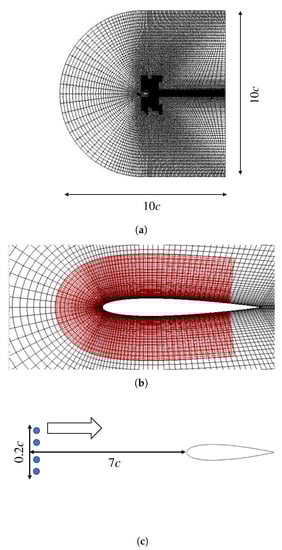
Figure 1.
Computational domain and grid for the NACA0012 icing simulation: (a) complete domain; (b) zoomed-in view around the wing (the main and sub grids are shown in black and red, respectively); (c) initial position of droplets.
Table 1 summarizes the computational conditions that were set with reference to an experiment performed by Anderson and Tsao []. In the simulation, the exposure time was divided into quarters, and steps 2 to 5 of the numerical procedure, as discussed in Section 2, were repeated four times. As summarized in Table 2, four simulation cases were considered to evaluate the influence of each phenomenon on the icing process.

Table 1.
Numerical conditions for the NACA0012 icing simulation.
Table 2.
Computational cases for NACA0012 icing simulation.
Figure 2 shows the results for the ice shape and collection efficiency . The impinged mass , which is defined in Equation (19), is computed using the following equation, with reference to :
and this mass is a key factor to determine the ice shape.
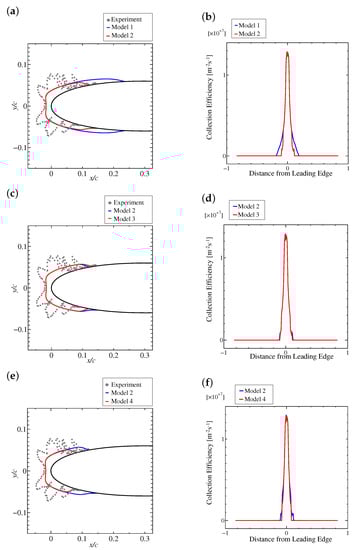
Figure 2.
Comparison of ice shapes and collection efficiency for different SLD models: (a,b), Models 1 and 2; (c,d), Models 2 and 3; (e,f), Models 2 and 4.
Figure 2a presents a comparison of the ice shape, in which the coordinate systems are non-dimensionalized using the chord length of the airfoil, c. The ice shape covers the leading edge of the airfoil. Under real and experimental conditions, however, the ice shape is extremely complex and cannot be easily reproduced using the present simulation. Therefore, instead of reproducing the ice shape, we focus on the icing area because it is a key parameter for the design of anti-icing devices for the airfoil. In Model 2 (i.e., the splash-bounce model), the icing area becomes narrow, and the limitation location of the icing moves toward the leading edge. Figure 2b shows the collection efficiency at the final step of the four steps. The horizontal axis represents the distance from the leading edge of the airfoil non-dimensionalized by c. The positive and negative values of the horizontal axis represent the location of the airfoil on the suction (upper) and pressure (lower) surfaces, respectively. Because the AoA is zero, the collection efficiency is maximized around the leading edge. In Model 2, the region of the non-zero collection efficiency becomes narrow, and it corresponds to the iced area.
Figure 2c,d show the ice shape and collection coefficient pertaining to Model 3 (deformation model). Owing to the insignificant difference between Models 1 and 3, the influence of the deformation can be considered to be extremely small in the icing process.
The effect of the breakup phenomenon is shown in Figure 2e,f. In Model 4 (breakup model), the icing limitation moves toward the leading edge, and the icing decreases. The iced region is in better agreement with the experimentally obtained region compared to that in the other cases. The droplet collection efficiency decreases in the regions farther from the leading edge when considering the breakup phenomenon. Therefore, the impingement characteristics change owing to the breakup of the droplets, and the icing limit changes with the increase in the intensity of the splash and bounce phenomena. Accordingly, in the SLD simulation, the splash-bounce model and the breakup model yield a reasonable icing area, and the effect of the deformation is minimal.
4. Icing Simulation for Axial Fan
A three-dimensional SLD icing simulation for a commercial axial fan (Kairyu series A2D6H-411, Showa Denki Co., Osaka, Japan ) was performed. Although the axial fan has 12 rotor blades, only one blade was examined to simplify the problem. At the inlet boundary, the velocity and total temperature were fixed, and the Mach number was extrapolated. The periodic boundary condition was imposed in the circumferential direction. At the inlet boundary, the velocity and total temperature were fixed, and the Mach number was extrapolated. At the outlet boundary, the static pressure was fixed. A non-slip and static temperature were imposed on the blade surface. The overset grid method was used to improve the computational accuracy, with the total grid points being approximately 6 million, as shown in Figure 3. The computational conditions are summarized in Table 3. This method has been validated in our previous study [], in which the icing and shedding for the MVD of 30 μm was examined. The total exposure time was 15 s. Three computational cycles were performed, with the exposure time for one cycle being 5 s.
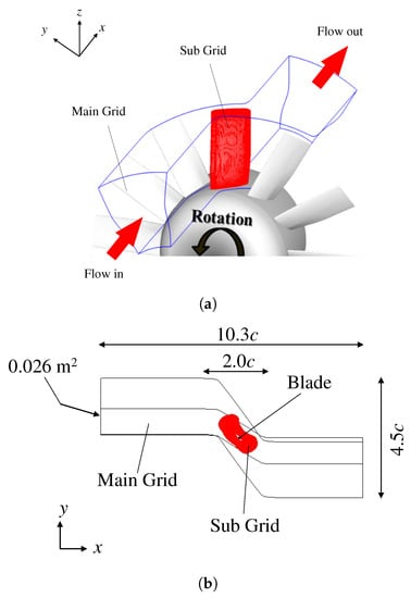
Figure 3.
Flow around axial fan and computational domain: the main and sub grids are shown in blue and red, respectively. (a) Overview and (b) top view of the computational grid.
Table 3.
Numerical conditions for the axial fan icing simulation.
Four different cases, as summarized in Table 4, were examined to verify the effect of the SLD model and the temperature of the droplets on the icing. In general, the surface tension and viscosity of the SLD vary owing to the temperature of the droplet; therefore, the temperature affects not only the icing phenomenon but also the SLD behavior. The decrease in the SLD temperature corresponds to an increase in the surface tension and viscosity, as shown in Equations (6) and (8), respectively.
Table 4.
Computational conditions for axial fan icing.
Figure 4 shows the comparison of the effect of the SLD models (splash-bounce, deformation, and breakup) on for the blade surface. The leading and trailing edges are represented as “L.E.” and “T.E.”, respectively. Figure 4a,b show the values of on the pressure and suction surfaces in Case 1, in which the SLD model is not considered. The maximum value of occurs around the leading edge because the droplet directly impinges and adheres to this area. On the pressure side, the values are distributed on the entire surface, and increases at the region close to the hub and trailing edge. On the suction side, is extremely small. Figure 4c,d show the pertaining to the SLD model of Case 2. The distribution is highly similar to that shown in Figure 4a,b. The values are distributed at the region near not only the hub but also the tip on the pressure side. On the suction side, is very small.
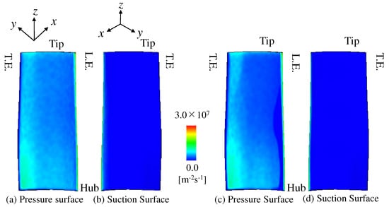
Figure 4.
Collection efficiency: (a,b) w/o SLD model (Case 1) and (c,d) w/ SLD model (Case 2).
Next, we discuss the influence of the number of SLD in each event listed in Table 5. The ratio of the number of SLDs in each event to the total number of SLDs is defined as
Table 5.
Effect of the SLD model and temperature on each event.
The number of total SLDs is denoted as , and the number of SLDs in each event is denoted as ; event here refers to splash, bounce, and adherence.
In Case 1, the number of adhered particles is 40.3% the total number of SLDs, and only adherence occurs since the splash-bounce model is absent. In contrast, when considering the SLD model, decreases, whereas and appear. Moreover, is smaller than . Therefore, the number of adhered particles decreases by 7.3%. Owing to the similar distributions in Cases 2 and 3, the difference in the collection efficiency distribution, as shown in Figure 4, pertains to the consideration of the splash-bounce model. Moreover, the number of deformed and broken particles is negligibly small. These results indicate that, although the influence of the deformation and breakup events is extremely small, the splash-bounce phenomenon considered influences the icing process. In Case 4, the droplet temperature decreases, and increases; however, and decrease owing to the change in the physical properties. Therefore, we further examined the icing phenomenon considering the splash-bounce model without the deformation and breakup models (Cases 1, 3, and 4).
Figure 5 shows the ice thickness on the pressure surface for each case. As discussed, the icing tends to occur in the pressure surface and not on the suction surface. The maximum ice thickness occurs at the leading edge (approximately 1.2 mm in Cases 1 and 3 and 1.5 mm in Case 4). In Case 1, as shown in Figure 5a, the icing covers the complete surface owing to the absence of the splash-bounce model. In Case 3, the ice thickness is smaller than that in Case 1 in the region close to the leading edge, and the thickness increases closer to the trailing edge owing to the bouncing of the SLD at the leading edge. This phenomenon is especially notable in Case 4.
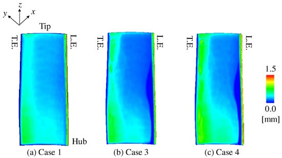
Figure 5.
Ice thickness distribution on the pressure surface: (a) Case 1, (b) Case 3, and (c) Case 4.
Figure 6a shows the flow field in terms of the Mach number at 90% span of the blade without the icing (i.e., before icing) for Case 3. In the suction side, flow separation occurs in the region close to the trailing edge. Figure 6b shows the flow field after the icing, that is, corresponding to the icing distribution at 15.0 s. The iced region (shown in black) appears around the leading and trailing edges on the pressure surface. The flow separation region expands owing to the icing.

Figure 6.
Mach number distribution at 90% span of the fan for Case 3.
Moreover, we discuss the time variation of the loss of the mass flow rate. The reduction rate of flow is defined in terms of the flow rate Q, as
Here, and denote the mass flow rate before and after icing, respectively. Q is defined as
where is the cross-sectional area of the flow passage, is the surface area vector, and is the local density of the fluid. As time advances, the ice grows, and it disturbs and blocks the flow. Therefore, increases with time; specifically, , , , and at 15 s, 30 s, 45 s, and 60 s, respectively. If the exposure time is sufficiently large, there is considerable ice growth, and it may be peeled off from the blade. Such ice shedding can critically damage the engine material and components. However, in this study, the exposure time was too small to reproduce the ice shedding owing to the limitations of the computational cost. This phenomenon must be addressed in future research.
Figure 7 shows the ice shape around the leading edge at the midspan of the blade. Figure 7a presents a comparison of the effects of the SLD model on the ice shape, i.e., Cases 1 and 3. The icing occurs at the leading edge in Case 3, whereas the icing region expands in Case 1, as indicated by the red circle. These findings are in agreement with the ice thickness distribution, as shown in Figure 5a,b. Figure 7b shows the effect of the SLD temperature on the ice shape, i.e., Cases 3 and 4. In Case 3, the icing occurs at not only the leading edge (circled in black) but also the suction () side. The ice on the suction side close to the leading edge is the glaze ice generated by the water-runback (circled in blue), which occurs because the SLD temperature is relatively higher than that in Case 4. In Case 4, the ice at the leading edge thickens (circled in black) owing to the presence of rime ice; specifically, the SLD instantaneously freezes when the droplet collides on the surface. This phenomenon occurs because the water-runback and splash-bounce phenomena do not occur. In addition, the icing on the pressure side does not occur in both the cases, as shown by the red circle.
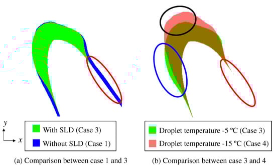
Figure 7.
Ice shape around the leading edge at the midspan.
5. Conclusions
Icing simulations were performed considering the specific phenomena of SLDs i.e., splash, bounce, deformation, and breakup.
The results of the SLD simulation for NACA0012 were in reasonable agreement with the experimental data in terms of the ice shape. The effect of the computational models of the SLD-specific phenomena on the icing was clarified. Specifically, the splash and bounce events considerably influence the icing phenomena, whereas the effects of deformation are negligibly small.
In the SLD icing simulation considering the axial fan, when the SLD-specific phenomena were taken into account, the collection efficiency was observed to be distributed at the region near not only the hub but also the tip on the pressure side. The SLD icing thus affected the flow field around the fan blade, and flow separation was observed behind the icing layer. Moreover, the ice thickness around the leading edge when the SLD-phenomena was considered was smaller than that when not considering the SLD phenomena, and the ice thickness was noted to increase toward the trailing edge. With the decrease in the droplet temperature, the number of droplets adhering on the blade increased, and the number of droplets that splashed and bounced decreased.
Author Contributions
Conceptualization, T.T. and M.Y.; methodology, T.T. and M.Y.; validation, T.T., K.F., H.M. and M.Y.; formal analysis, T.T.; investigation, T.T., K.F., H.M. and M.Y.; writing—original draft preparation, T.T.; writing—review and editing, K.F., H.M., N.F. and M.Y.; visualization, T.T.; supervision, M.Y.; project administration, M.Y.; funding acquisition, M.Y. All authors have read and agreed to the published version of the manuscript.
Funding
This research was partially supported by the Ministry of Education, Culture, Sports, Science and Technology through a Grant-in-Aid for Scientific Research (B) (Grant No. 16H03918).
Acknowledgments
The authors are grateful to Miki Shimura, former graduate school student of the Tokyo University of Science, for her pioneering research.
Conflicts of Interest
The authors declare no conflict of interest.
Abbreviations
The following abbreviations are used in this manuscript:
| LWC | Liquid water content |
| MVD | Median volume diameter |
| SLD | Super-cooled large droplet |
References
- Zhang, X.; Min, J.; Wu, X. Model for aircraft icing with consideration of property-variable rime ice. Int. J. Heat Mass Transf. 2016, 97, 185–190. [Google Scholar] [CrossRef]
- Fortin, G.; Ilinca, A.; Laforte, J.L.; Brandi, V. A new roughness computation method and geometric accretion model for airfoil icing. J. Aircr. 2004, 41, 119–127. [Google Scholar] [CrossRef]
- Janjua, Z.A.; Turnbull, B.; Hibberd, S.; Choi, K.S. Mixed ice accretion on aircraft wings. Phys. Fluids 2018, 30, 027101. [Google Scholar] [CrossRef]
- Szilder, K.; Lozowski, E.P. Progress Towards a 3D Numerical Simulation of Ice Accretion on a Swept Wing Using the Morphogenetic Approach; SAE Technical Paper, No. 2015-01-2162; SAE: Warrendale, PA, USA, 2015. [Google Scholar]
- Szilder, K.; Yuan, W. In-flight icing on unmanned aerial vehicle and its aerodynamic penalties. Prog. Flight Phys. 2017, 9, 173–188. [Google Scholar]
- Shen, X.; Lin, G.; Yu, J.; Du, C. Three-dimensional numerical simulation of ice accretion at the engine inlet. J. Aircr. 2013, 50, 635–642. [Google Scholar] [CrossRef]
- Wang, Z.; Zhu, C. Study of the effect of centrifugal force on rotor blade icing process. Int. J. Aerosp. Eng. 2017, 2017, 8695170. [Google Scholar] [CrossRef]
- Narducci, R.; Kreeger, R.E. Analysis of a Hovering Rotor in Icing Conditions; NASA-TM217126; NASA: Washington, DC, USA, 2012.
- Mingione, G.; Brandi, V. Ice accretion prediction on multielement airfoils. J. Aircr. 1998, 35, 240–246. [Google Scholar] [CrossRef]
- Wright, W.B.; Potapczuk, M.G. Computational simulation for large droplet icing. In Proceedings of the FAA International Conference on Aircraft Inflight Icing, Springfield, VA, USA, 6–8 May 1996; Report No. DOT/FAA/AR-96/81. Volume II, pp. 545–555. [Google Scholar]
- Zhang, C.; Liu, H. Effect of drop size on the impact thermodynamics for supercooled large droplet in aircraft icing. Phys. Fluids 2016, 28, 062107. [Google Scholar] [CrossRef]
- Wang, C.; Chang, S.; Hongwei, W. Lagrangian approach for simulating supercooled large droplets’ impingement effect. J. Aircr. 2015, 52, 524–537. [Google Scholar] [CrossRef]
- Wang, C.; Chang, S.; Leng, M.; Yang, B. A two-dimensional splashing model for investigating impingement characteristics of supercooled large droplets. Int. J. Multiph. Flow 2016, 80, 131–149. [Google Scholar] [CrossRef]
- Honsek, R.; Habashi, W.G.; Aube, M.S. Eulerian modeling of in-flight icing due to supercooled large droplets. J. Aircr. 2008, 45, 1290–1296. [Google Scholar] [CrossRef]
- Bilodeau, D.R. Eulerian modeling of supercooled large droplet splashing and bouncing. J. Aircr. 2015, 52, 1611–1624. [Google Scholar] [CrossRef]
- Raj, L.P.; Lee, J.W.; Myong, R.S. Ice accretion and aerodynamic effects on a multi-element airfoil under SLD icing conditions. Aerosp. Sci. Technol. 2019, 85, 320–333. [Google Scholar]
- Cao, Y.; Xin, M. Numerical simulation of supercooled large droplet icing phenomenon: A Review. Arch. Comput. Methods Eng. 2019. [Google Scholar] [CrossRef]
- Hayashi, R.; Yamamoto, M. Numerical Simulation on Ice Shedding Phenomena in Turbomachinery. J. Energy Power Eng. 2015, 9, 45–53. [Google Scholar]
- Yee, H.C. Upwind and Symmetric Shock-Capturing Schemes; NASA-TM-89464; NASA: Washington, DC, USA, 1987.
- Fujii, K.; Obayashi, S. Practical Applications of New LU-ADI Scheme for the Three-Dimensional Navier–Stokes Computation of Transonic Viscous Flows; AIAA Paper 86-0513; AIAA: Reston, VA, USA, 1986. [Google Scholar]
- Kato, M.; Launder, B.E. The modeling of turbulent flow around stationary and vibrating square cylinders. In Proceedings of the 9th Symposium on Turbulent Shear Flows, Kyoto, Japan, 16–18 August 1993; Volume 1, pp. 10–14. [Google Scholar]
- Clift, R.; Grace, J.R.; Weber, M.E. Bubbles, Drops and Particles; Academic Press: Cambridge, MA, USA, 1978. [Google Scholar]
- Luxford, G. Experimental and Modelling Investigation of the Deformation, Drag and Break-Up of Drizzle Droplets Subjected to Strong Aerodynamics Forces in Relation to SLD Aircraft Icing. Ph.D. Thesis, Cranfield University School of Engineering, Bedford, UK, 2005. [Google Scholar]
- Hsiang, L.P.; Faeth, G. Secondary drop breakup in the deformation regime. In Proceedings of the 30th AIAA Aerospace Sciences Meeting and Exhibit, Reno, NV, USA, 6–9 January 1992; p. 110. [Google Scholar]
- Wright, W.B. Further Refinement of the LEWICE SLD Model; NASA TM-214132; NASA: Washington, DC, USA, 2006; 29p.
- Wright, W.B.; Potapczuk, M.; Levinson, L. Comparison of LEWICE and GlennICE in the SLD Regime; NASA TM-215174; NASA: Washington, DC, USA, 2008; 31p.
- Özgen, S.; Canibek, M. Ice accretion simulation on multi-element airfoils using extended Messinger model. J. Heat Mass Transf. 2009, 45, 305. [Google Scholar] [CrossRef]
- Anderson, D.N.; Tsao, J.C. Ice Shape Scaling for Aircraft in SLD Conditions; NASA CR-215302; NASA: Washington, DC, USA, 2008.
© 2020 by the authors. Licensee MDPI, Basel, Switzerland. This article is an open access article distributed under the terms and conditions of the Creative Commons Attribution (CC BY) license (http://creativecommons.org/licenses/by/4.0/).