Unsteady Lift Prediction with a Higher-Order Potential Flow Method

Abstract

An unsteady formulation of the Kutta–Joukowski theorem has been used with a higher-order potential flow method for the prediction of three-dimensional unsteady lift. This study describes the implementation and verification of the approach in detail sufficient for reproduction by future developers. Verification was conducted using the classical responses to a two-dimensional airfoil entering a sharp-edged gust and a sinusoidal gust with errors of less than 1% for both. The method was then compared with the three-dimensional unsteady lift response of a wing as modeled in two unsteady vortex-lattice methods. Results showed agreement in peak lift coefficient prediction to within 1% and 7%, respectively, and mean agreement within 0.25% for the full response.

1. Introduction

1.1. Motivation

In previous work [1,2,3,4], the authors developed a time-stepping potential flow method that uses higher-order vorticity elements to represent lifting surfaces and wakes. Although all results discussed in previous work were either steady or quasi-steady and time-averaged, the method is capable of quasi-steady time-accurate analysis. By “quasi-steady”, the authors refer to the enforcement of flow tangency boundary conditions based on the time-accurate flow field at each time step and the subsequent propagation of the resulting vorticity distribution of the lifting surfaces throughout the wake. To determine a fully unsteady lift response, the influence of shed vorticity due to changes in lift (also referred to as “shed circulation” [5]) and apparent mass effects must also be taken into account [5,6,7].

The use of an unsteady formulation of the Kutta–Joukowski theorem was suggested by Drela [8] as a fast approach to predict unsteady lift for the purpose of an integrated aerodynamic, structural, and control model simulation of highly-flexible aircraft. This approach has also been referred to as the Joukowski theorem, as by Simpson et al. [9]. The simplicity of this technique, along with the authors’ previous use of the Kutta–Joukowski theorem for steady and quasi-steady lift prediction, make it an appealing solution for the prediction of unsteady lift within the potential flow method.

Few details are available in the literature regarding the implementation and verification of an unsteady formulation of the Kutta–Joukowski theorem within a potential flow method. The objective of this note is to provide future developers with a comprehensive example of such an implementation within the authors’ higher-order potential flow method. In particular, emphasis is placed on identifying the influence of the numerical discretization approach on lift prediction of classical verification cases. The quasi-steady (kinematics only), shed-circulation, and fully unsteady responses are also provided for each case to elucidate the effect of each term and to provide future developers with information to aid in troubleshooting and debugging.

1.2. Background on Unsteady Lift Prediction

In order to support the use of the unsteady formulation of the Kutta–Joukowski theorem, it is helpful to begin with a broader discussion of approaches to the calculation of unsteady lift. The lifting surfaces under consideration are assumed to be at low Mach number and low to moderate angles of attack. As such, the discussion that follows is limited to unsteady lift predictions for incompressible, attached flow systems under general gust loadings.

In the calculation of unsteady lift, one of two approaches is typically applied—pressure integration [6] or the indicial response method [5,10]. Pressure integration is the determination of the lift force through integration of the local pressures on the surface of the wing. The indicial response method, as is found in rotorcraft analysis methods such as RCAS [11] and CAMRAD [12,13], assumes the form of the response to a step change in a set of aerodynamic boundary conditions. For example, the classical solution for a step change in angle of attack of an airfoil in an incompressible flow is the Wagner function [14], which assumes the circulatory unsteady lift response (including vorticity on the surface and shed into the wake) based on unsteady two-dimensional thin airfoil theory. This solution can then be superimposed over time in order to estimate the two-dimensional, circulatory, unsteady-lift response that is due to a series of changes in angle of attack using the Duhamel integral. For the case of arbitrary changes in angle of attack, the Duhamel integral must be numerically integrated. A relation exists between the two approaches in that the indicial response can be found via pressure integration, but the actual method itself is independent of the way that the response is developed.

The pressure integration method and the indicial response method vary from one another in terms of the assumptions applied and the requirements with respect to the flow-field modeling. The first notable difference comes with respect to the treatment of shed vorticity resulting from changes in lift. In order to successfully predict unsteady lift through pressure integration, the flow-field model must include the vortices shed into the wake due to changes in lift. Assumptions regarding the motion of these vortices may vary, e.g., the motion can be prescribed as in fixed wakes or be determined at each time step based on locally induced velocities as in relaxed wakes. In either case, the velocities induced by the vortices on the lifting surface are the physical mechanism for the unsteady lift response, thus, it is essential that they are taken into account. Alternatively, to predict the unsteady lift using an indicial response method, the shed vorticity must not be present in the flow-field in order to prevent it from being double counted. The location of the shed vorticity is thus assumed within the indicial response.

The second notable difference is that in most applications, the indicial response approach is in essence a strip method. As such, it assumes that each section of a lifting surface behaves as a two-dimensional airfoil. This is akin to a high aspect-ratio assumption for a steady, fixed-wing analysis. In the case of unsteady analysis, it also indicates that a segment of the shed vorticity at one spanwise location directly aft of the lifting surface has no influence on the lift of a neighboring section. The pressure integration approach does not have this limitation and, as a result, is capable of accounting for three-dimensional effects as long as the underlying model can support such a method.

An exception exists to the limitation on use of indicial responses with respect to capturing three-dimensional effects. It is possible to compute a three-dimensional unsteady solution which is “sliced” into spanwise segments used in order to obtain two-dimensional responses. These responses can then later be combined with local angle of attack history within the Duhamel integral to account for three-dimensional unsteady wake effects. An example of this type of analysis can be found in Kitson et al. [15] for modeling flexible, high-aspect ratio wings.

A final difference between the two approaches is in their respective reliance on the model fidelity relative to the physical system. Unsteady lift predictions through pressure integration depend directly on the quality of the geometric representation of the lifting surface and the location and strength of the shed vortices in the wake. Alternatively, indicial methods depend only on the time history of the variation in angle of attack. While the fidelity of the model has an influence on the accuracy of this time history, the model fidelity is separated from the calculation of the unsteady lift itself.

To put the unsteady Kutta–Joukowski formulation in context with these methods, it is helpful to consider the formulation. According to Drela [8], the vector form of the unsteady Kutta–Joukowski theorem to be evaluated at each time step is

$${\overline{F}}_L^{\prime }=\rho \Gamma \overline{V}\times \hat{s}+\rho \frac{\partial \Gamma }{\partial t}\frac{c}{|{\overline{V}}_{\perp }|}\overline{V}\times \hat{s}$$

(1)

where ${\overline{F}}_L^{\prime }$ is the lift per unit span, $\overline{V}$ is the relative velocity evaluated at the quarter chord location, and $\Gamma$ is the local circulation oriented along the unit vector $\hat{s}$. The component of the relative velocity that is perpendicular to the circulation, ${\overline{V}}_{\perp }$, is given by

$${\overline{V}}_{\perp }=\overline{V}-(\overline{V}·\hat{s})\hat{s}$$

(2)

Because the circulation as a function of time is determined through the enforcement of flow tangency on the lifting surfaces based on the time-accurate flow-field, this approach depends both on the geometry of the lifting surfaces and an accurate assessment of the local velocities. As a result, in comparison with pressure integration and indicial methods, the approach is more closely related to a pressure integration due to this reliance on the local velocities. In fact, a comparison of the results of these two methods when applied to a flat plate that is at an angle of attack reveals that the main difference is that the Kutta–Joukowski approach implicitly accounts for the leading-edge suction force, which is omitted in the pressure integration on a flat plate [3].

In order to improve the computational efficiency, in some cases the Kutta–Joukowski method can be supplemented with elements from the indicial approach. For example, in his application, Drela [8] accounted for the influence of shed vorticity through an empirical lag term based on thin-airfoil theory results, rather than through a direct calculation of induced velocity. The use of this term is reminiscent of an indicial method, as it omits tracking of the shed vorticity.

2. Method

The method of analysis for this study is an incompressible, potential flow formulation composed of higher-order singularity elements, the strengths of which are determined through the application of the Neumann (flow-tangency) boundary conditions. A general overview of the approach is provided here. For further details, the reader is referred to Bramesfeld and Maughmer [2] and Cole et al. [4].

According to Katz and Plotkin [6], higher-order potential flow solutions are built with elements that consist of “higher-order” distributions of singularity strengths to represent lifting surfaces and their wakes. In this context, “higher-order” refers to the order of polynomial used to represent the singularity distribution on each panel. In contrast, a vortex-lattice method would be zeroth order. The higher-order singularity elements used in this case are referred to as “distributed vorticity elements” or DVEs [1,2]. These elements, as depicted in Figure 1, consist of leading-edge and trailing-edge vortices (indicated by ${\Gamma }_{l.e.}$ and ${\Gamma }_{t.e.}$, respectively) that have quadratic circulation distributions in the spanwise ($\eta$) direction. The leading- and trailing-edge vortices are connected in the streamwise ($\xi$) direction by a vortex sheet that has a linearly changing distribution of vorticity strength (indicated by $\gamma$) in the spanwise ($\eta$) direction.

Lifting surfaces are represented within the method using surface DVEs (SDVEs). Spanwise rows of these elements form lifting lines with bound circulations whose strength changes as second-order splines in the spanwise direction. The Neumann (flow tangency) boundary condition is enforced at control points and transitional conditions for circulation and vorticity between neighboring DVEs are applied in order to solve for the strength distribution (A, B, and C coefficients) of the bound circulation.

The wake of each lifting surface is developed using a time-stepping approach. During each time step, the lifting surface is advanced by a spatial increment and a row of DVEs is passed into the wake bridging the gap between the wing-trailing edge and the wake elements of the previous time steps. If the wake is assumed to be quasi-steady, the trailing vorticity shed from the lifting surface at each time step is propagated throughout the wake. In this case, the leading-edge and trailing-edge filaments of the wake DVEs are omitted from the calculation as they are equal in magnitude and opposite in direction. If a fully unsteady analysis is desired, the strength of each wake DVE remains constant at the value at the instant when it was passed into the wake initially. As a result, the leading- and trailing-edge filaments must be retained in the calculation. Although the original method has numerically stable wake relaxation capabilities, the added leading- and trailing-edge filaments introduce the potential for large induced velocities in the wake. The wake is thus assumed to be fixed for all analysis in this study to prevent numerical instabilities in the wake relaxation process.

Treating each SDVE as an individual lifting line with Equation (1), the freestream (kinematic) lift force may be calculated for m lifting lines and n spanwise panels as

$${\displaystyle {\overline{F}}_L=\rho {\sum }_{i=1}^m{\sum }_{j=1}^n\underset{-{\eta }_{i,j}}{\overset{{\eta }_{i,j}}{\int }}\left[|{\overline{V}}_{\infty }\times \widehat{s_{i,j}}|\left({\Gamma }_{i,j}\left(\eta \right)-\left\{\begin{array}{cc}0,& i=1\\ {\Gamma }_{i-1,j}\left(\eta \right),& i>1\end{array}\right\}\right)+\frac{\partial {\Gamma }_{i,j}\left(\eta \right)}{\partial t}\left(2{\xi }_{i,j}\right)\right]\left(\frac{{\overline{V}}_{\infty }\times \widehat{s_{i,j}}}{|{\overline{V}}_{\infty }\times \widehat{s_{i,j}}|}\right)d\eta }$$

(3)

where $\hat{s}$ is the unit vector in the global reference frame along the leading-edge bound vortex of the DVE. In this way, the local lift of each DVE is resolved in the global reference frame such that the contributions can be summed. The forces due to induced velocities in the freestream direction are calculated in a similar manner and summed with the true freestream lift forces to determine the total lift force. Finally, the $\partial \Gamma /\partial t$ term is estimated using standard numerical differentiation techniques. For example, it can be estimated using backwards differencing as the change in chordwise integrated circulation at each SDVE divided by the time-step size.

3. Results

3.1. Panel and Time-Step Size Constraint

To achieve numerical convergence of the method, a constraint is necessary on the ratio of the distance traversed by a single point on the wing over a time-step is defined by $\Delta x_w$ and the length of an SDVE is dictated by $\Delta x_c$:

$$\frac{\Delta x_w}{\Delta x_c}=1.$$

(4)

This constraint is suggested for use with unsteady vortex-lattice methods by Simpson and Palacios [16] and is attributed to a desire to ensure that the trailing edge panels and shed wake panels have equal areas.

Omission of this constraint results in significant discontinuities in the fully unsteady lift response to a sharp-edged gust. A physical explanation for this effect can be made based on the unsteady lift equation (Equation (3)). The term that results in the discontinuity is the $\partial \Gamma /\partial t$ term. This term is akin to the time derivative of the velocity potential ($d\varphi /dt$) in the unsteady Bernoulli equation, which accounts for the non-circulatory lift [3]. In the higher-order fixed-wake setting, the $\partial \Gamma /\partial t$ term is a spatial integration of a time derivative of an impulse function. The time derivative is estimated by taking the difference in integrated circulation over two time-steps as described previously, but the actual change in integrated circulation occurs at a single point on the DVE (the leading edge) and is controlled by the conditions at a single point on the DVE (the control point). As a result, no matter how small the time step is, the change in circulation is the same as long as the conditions at the control point dictate a change. Thus, $\partial \Gamma /\partial t$ will tend towards infinity with decreasing time-step size relative to the length of the SDVE. Likewise, $\partial \Gamma /\partial t$ will tend towards zero with increasing time-step size for the same event. The only time-step size that makes it so that the estimated $\partial \Gamma /\partial t$ term is assuredly in the correct range is that which forces the change on the control point to have happened within the distance traversed by the control point over the last time-step. To ensure this is the case, the constraint provided in Equation (4) must be applied.

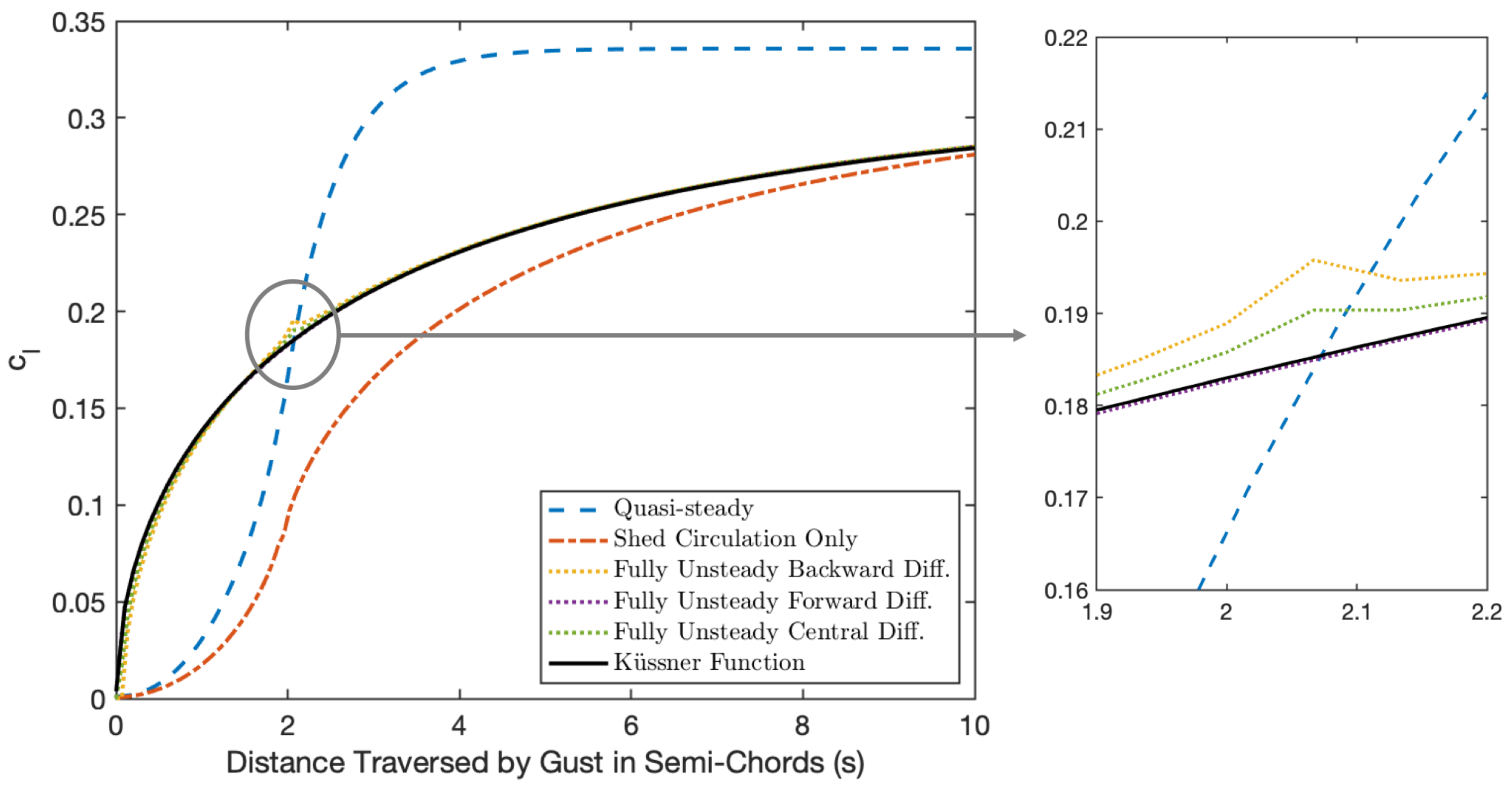
3.2. Sharp-Edged Gust Verification

In order to verify that the described method correctly accounts for the variations in local velocity experienced by a wing, the first case considered is an airfoil encountering a vertical sharp-edged gust. The lift response of a thin, two-dimensional airfoil entering a vertical sharp-edged gust of small magnitude, $w_0$, relative to the freestream velocity, $V_{\infty }$, i.e., $w_0/V_{\infty }<<1$ was solved by von Kármán and Sears [5,17,18]. According to this theory, the two-dimensional lift coefficient response ($c_l\left(s\right)$) is given by

$$c_l\left(s\right)=2\pi \left(\frac{w_0}{V_{\infty }}\right)\psi \left(s\right),$$

(5)

where $\psi$ is the Küssner function. The Küssner function as formulated by Kayran [19] varies with the location of the gust in semi-chords (s) as

$$\psi \left(s\right)=\frac{2}{\pi }{\int }_0^{\infty }\left(F\left(k\right)cos\left(k\right)+G\left(k\right)sin\left(k\right)\right)\frac{sin\left(ks\right)}{k}dk.$$

(6)

In Equation (6), F and G are the real and imaginary components of the Sears function as a function of the reduced frequency, k. Because Equation (6) does not have a closed form solution, it is numerically integrated for this application.

The sharp-edged gust was modeled in the higher-order potential flow method by applying symmetry boundary conditions (zero vorticity) to the tips of a finite wing, which results in an essentially two-dimensional analysis. The surface travels at a constant velocity in the global reference frame at an arbitrary very small angle of attack ($0.01°$) to allow for initialization of the wake. When it reaches a specified location in the global reference frame, it experiences a step change in the “induced” velocity on the surface of about 5% of the freestream velocity in the global z-direction. The magnitude of the step change (5% of the freestream) was selected such that the gust results in a measurable change in lift coefficient without violating the assumptions of the Küssner function (i.e., $w_0/V_{\infty }<<1$).

The lift response when 30 lifting lines are used with a time-step size scaled according to Equation (4) is shown in Figure 2 with forward, backward, and central differencing employed for the $\partial \Gamma /\partial t$ term. A discontinuity is visible in the fully unsteady response when backward differencing is used due to the lag in wake/lifting surface strengths, as is more clearly visible in the inset plot in Figure 2. On the time-step after the last control point on the surface experiences the gust, the $\partial \Gamma /\partial t$ term suddenly drops to zero on the lifting surface with backward differencing, but the shed circulation is still strongly influential. This problem can be solved by implementing forward differencing, effectively introducing a single time-step lead in the $\partial \Gamma /\partial t$ response such that it is in phase with the shed circulation response. Central differencing, while of a higher order of accuracy, does not fully account for this offset and thus the discontinuity remains. With forward differencing, the method is able to very closely match the lift response prediction using the Küssner function.

Also shown in Figure 2 is the unsteady response when the $\partial \Gamma /\partial t$ term, as implemented in the second integral in Equation (3), is omitted in order to characterize the relative magnitude of the unsteady terms. From this comparison, it is clear that it would be inappropriate to omit either of the unsteady terms in a gust response.

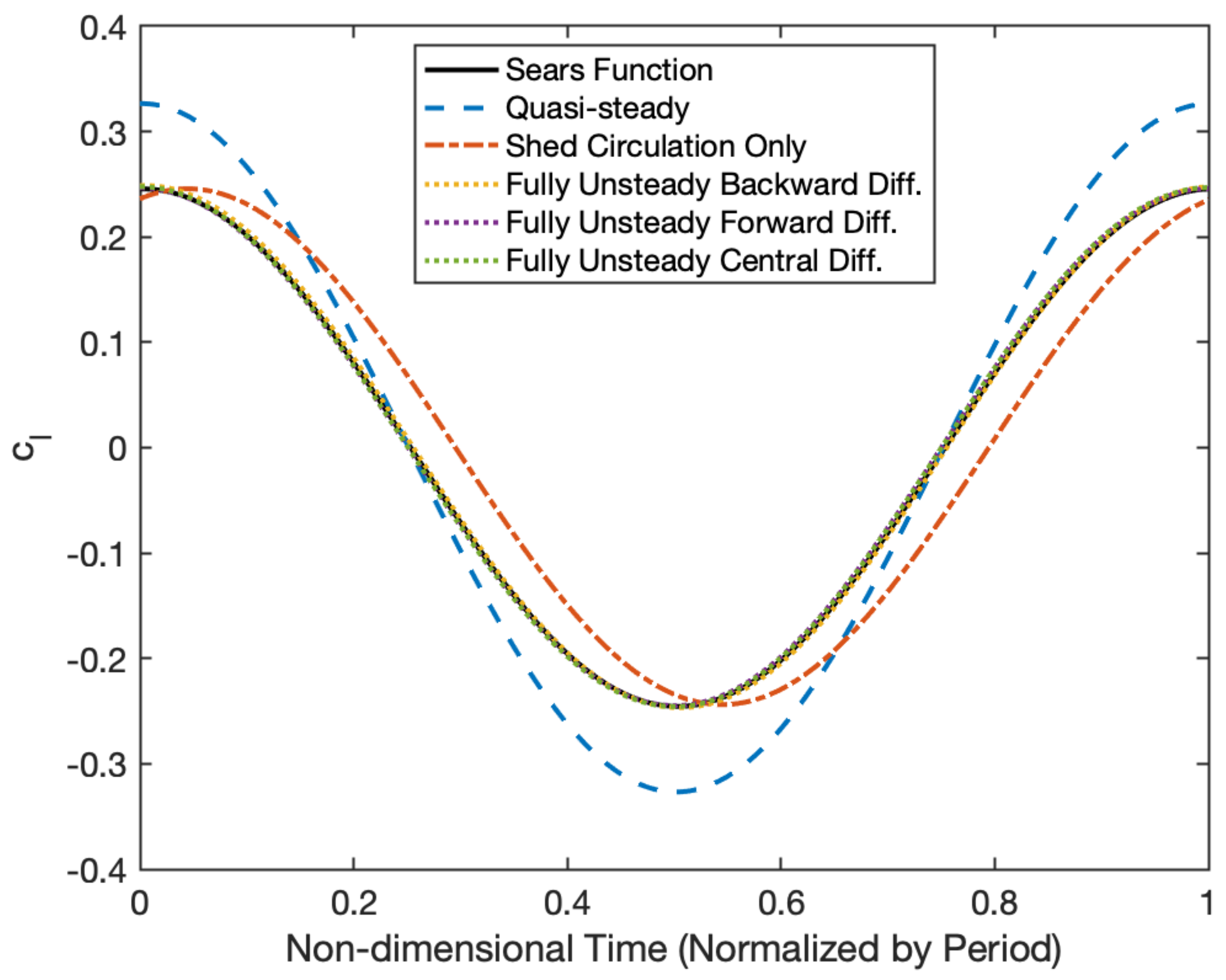
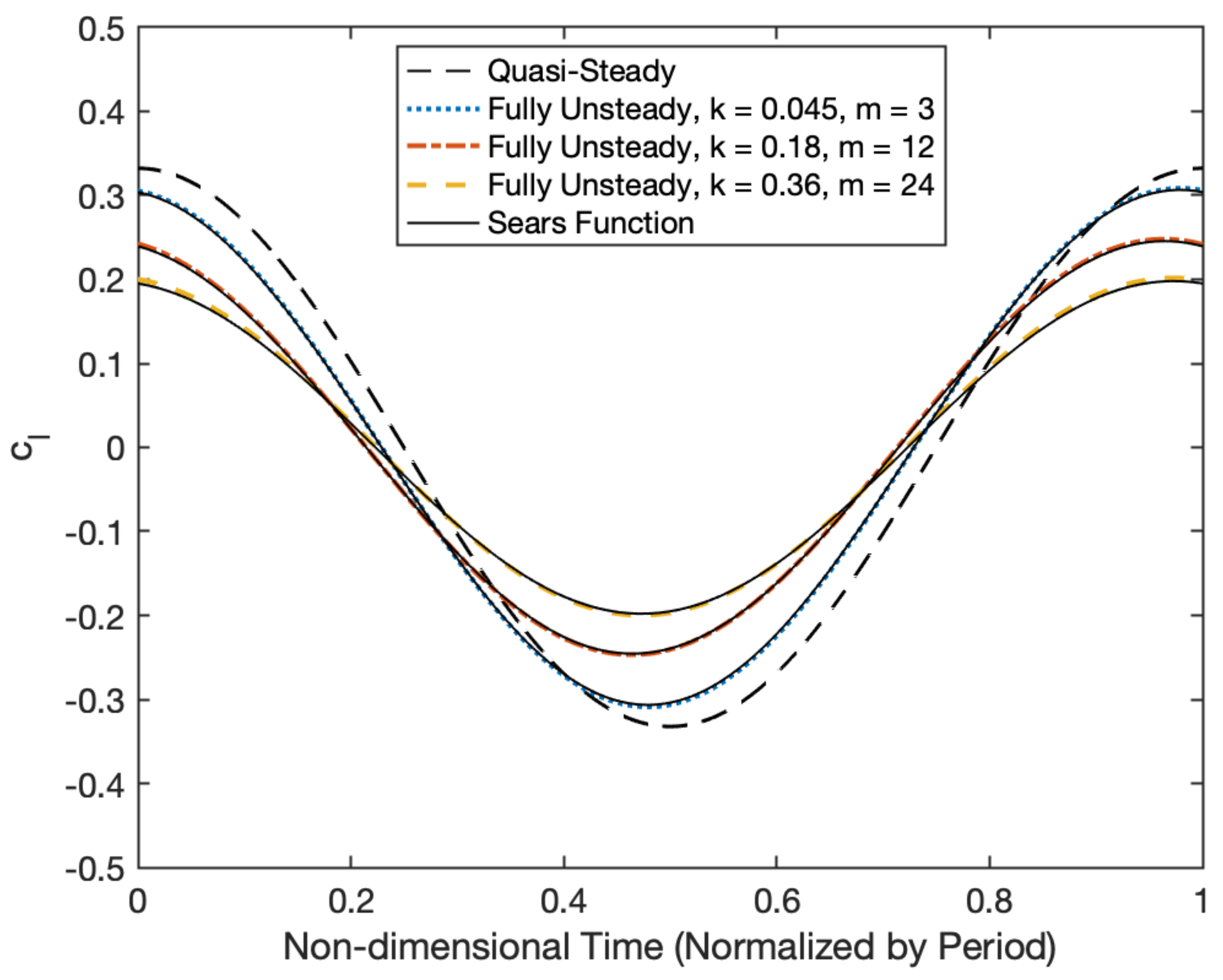
3.3. Sinusoidal Gust Verification

The lift response to a sinusoidal gust according to unsteady thin airfoil theory is given by

$$c_l\left(t\right)=2\pi \left(\frac{w_0}{V_{\infty }}\right)S\left(k\right)$$

(7)

where $w_0$ is the amplitude of the gust, $S\left(k\right)$ is the Sears function [17], and k is the reduced frequency. The reduced frequency is defined as

$$k=\frac{\omega c}{2V_{\infty }}$$

(8)

where $\omega$ is the frequency of the oscillation and c is the chord length.

To model this condition within the higher-order fixed-wake method, the z-component of the “induced” velocity was once again varied based on the x-location of each control point within the global reference frame. In this case, the amplitude of the variation was approximately 5% of the freestream and the frequency was varied to achieve reduced frequencies of 0.045 (quasi-steady), 0.18 (unsteady), and 0.36 (highly unsteady).

A comparison of the fully unsteady response with the quasi-steady and shed-circulation-only responses for the unsteady case ($k=0.18$) elucidates the influence of each term as shown in Figure 3. The quasi-steady response over-predicts the amplitude of the Sears function response. The addition of shed circulation damps this response (as in the sharp-edged gust response), but induces a phase-shift that is ultimately improved by the addition of the $\partial \Gamma /\partial t$ term. There is not a significant difference between the three discretization approaches, as would be intuitively expected due to both the smoothness of the velocity variations (in contrast to the sharp-edged gust) and the high time-step resolution at which the analysis was performed (approximately 200 time-steps per oscillation).

Comparisons of the lift response as calculated with the current approach and with unsteady thin-airfoil theory as a function of non-dimensional time are provided in Figure 4. These results are predicted with three chordwise panels in the quasi-steady case, twelve chordwise panels for the unsteady case, and 24 chordwise panels for the highly unsteady case with appropriately scaled time-steps. This resolution results in approximately 200 time-steps per oscillation for all three cases.

The predictions with the unsteady Kutta–Joukowski approach match the thin-airfoil-theory results well, as would be expected based on the step response and the assumptions of the model itself. The error in amplitude is less than 1% for all three cases. It is worth noting that a resolution of 200 time-steps per oscillation is not a universally applicable recommendation due to the interaction between the time and space discretization, and resolution studies are recommended on a case-by-case basis.

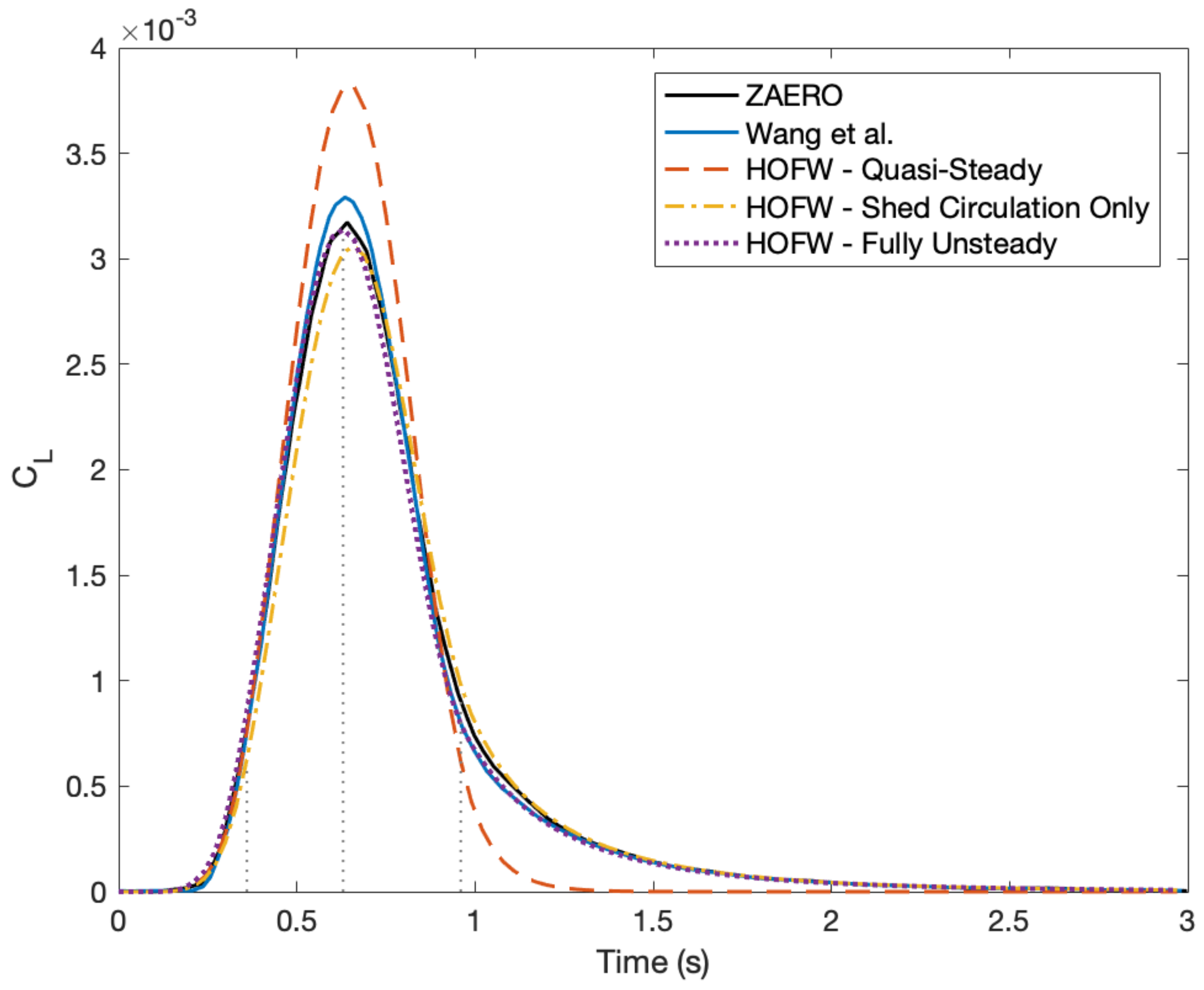
3.4. Finite Wing Comparison

While the previous results support the use of the method for two-dimensional unsteady lift predictions, the true strength of the higher-order method is in its application to lifting surfaces of finite spans. In addition, the implementation of the Kutta–Joukowski theorem as outlined in Equation (3) is three-dimensional in nature. Thus, it is important to compare predictions made with the method to other established methods for prediction of three-dimensional unsteady lift.

The case used for this purpose is that considered by Wang et al. [20], who considered the well-documented Goland wing [21] and provides results of two well-established unsteady vortex-lattice methods for comparison. The Goland wing is a rectangular wing with a half-span and chord of approximately 6.1 and 1.8 m, respectively [21]. Wang et al. [20] considered the wing traversing a 1-cosine gust that encompasses the full wing span. In this study, the freestream velocity was assumed to be 10 m/s with a gust amplitude of 0.01 m/s and gust length of four chord lengths.

The case considered by Wang et al. [20] was replicated in the current method with six chordwise elements, 15 spanwise elements, and a time-step size appropriate to satisfy the conditions outlined in Equation (4). Doubling the density of elements in the spanwise and chordwise direction changes the peak lift coefficient by less than 0.2%. Thus, six chordwise and 15 spanwise elements were deemed adequate.

The lift response as predicted by the higher-order fixed-wake (HOFW) method is shown in Figure 5 along with those predicted by the unsteady vortex-lattice method of Wang et al. [20] and the unsteady aerodynamic model in ZAERO [22], which is a commercially available aeroelastic analysis code. A 7% difference in the predicted peak lift coefficient is seen between the present method and Ref. [20] and a 1% difference between the present work and ZAERO. The remainder of the response is in good agreement, with a mean difference of less than 0.25%.

To elucidate the influence of each term on the lift response, the quasi-steady, shed circulation only and fully unsteady lift response are also provided Figure 5. The quasi-steady response both over-predicts the magnitude of the peak and the rate at which the lift returns to zero. The response prediction improves significantly with the addition of the influence of shed circulation, both in the magnitude of the peak and the rate of lift dissipation. This response slightly under-predicts the magnitude of the peak and lags behind the fully unsteady response. The phase shift in the circulation only response was also seen in the two-dimensional sinusoidal gust response (see Figure 3), although the change in peak magnitude was not. Thus, the $\partial \Gamma /\partial t$ term appears to shift the phase of the response in both two-dimensional and three-dimensional analysis, but to only influence the amplitude of the response in the three-dimensional analysis.

The spanwise lift distributions at three different instances in the gust encounter are provided in Figure 6 for both the shed circulation only (solid lines) and fully unsteady (dashed lines) responses. The vertical gray dotted lines in Figure 5 indicate the time instances for each lift distribution in Figure 6. The lag in the circulation only response is clear in the three time-steps in that at 0.36 s (prior to the peak lift coefficient), the fully unsteady lift is greater than the circulation only lift across the span. This effect then reverses at 0.96 s (after the peak lift coefficient), with the shed circulation lift exceeding the fully unsteady lift across the span. The spanwise distribution of the $\partial \Gamma /\partial t$ term is also visible in the figure as it is the difference between the shed circulation only response and the fully unsteady response at each time step. As per Equation (3), the sign and magnitude of this distribution is a function of the gradient in circulation with respect to time and can thus be resolved as a function of the spanwise location at the same resolution as the circulation distribution itself.

4. Conclusions

An unsteady formulation of the Kutta–Joukowski theorem has been used with a higher-order potential flow method for the prediction of three-dimensional unsteady lift. The approach has been verified with the classical responses to a two-dimensional airfoil entering a sharp-edged gust and a sinusoidal gust with errors of less than 1% for both. It was then compared with the three-dimensional unsteady lift response of a wing as modeled in two unsteady vortex-lattice methods. Results showed agreement in peak lift coefficient prediction to within 1% and 7%, respectively, and mean agreement within 0.25% for the full response.

Two points are noteworthy for future developers that are interested in implementing this approach. First, in order to capture the sharp-edged gust response, forward differencing in the $\partial \Gamma /\partial t$ term is necessary to avoid a discontinuity in the response when the gust reaches the trailing edge. Second, in all verification cases, both shed circulation and $\partial \Gamma /\partial t$ effects were necessary to correctly capture both the amplitude and phase of the response.

References

1. Bramesfeld, G. A Higher Order Vortex-Lattice Method with a Force-Free Wake. Ph.D. Thesis, The Pennsylvania State University, State College, PA, USA, 2006. [Google Scholar]
2. Bramesfeld, G.; Maughmer, M.D. Relaxed-Wake Vortex-Lattice Method Using Distributed Vorticity Elements. J. Aircr. 2008, 45, 560–568. [Google Scholar] [CrossRef]
3. Cole, J. A Higher-Order Free-Wake Method for Aerodynamic Performance Prediction of Propeller-Wing Systems. Ph.D. Thesis, The Pennsylvania State University, State College, PA, USA, 2016. [Google Scholar]
4. Cole, J.A.; Maughmer, M.D.; Kinzel, M.; Bramesfeld, G. Higher-Order Free-Wake Method for Propeller–Wing Systems. J. Aircr. 2019, 56, 150–165. [Google Scholar] [CrossRef]
5. Leishman, J. Principles of Helicopter Aerodynamics; Cambridge University Press: Cambridge, UK, 2006. [Google Scholar]
6. Katz, J.; Plotkin, A. Low-Speed Aerodynamics, 2nd ed.; Cambridge University Press: Cambridge, UK, 2001. [Google Scholar]
7. Drela, M. Flight Vehicle Aerodynamics; The MIT Press: Cambridge, MA, USA, 2014. [Google Scholar]
8. Drela, M. Integrated Simulation Model for Preliminary Aerodynamic, Structural, and Control-Law Design of Aircraft; AIAA Paper 99-1394; AIAA: Reston, VA, USA, 1999. [Google Scholar] [CrossRef] [Green Version]
9. Simpson, R.J.S.; Palacios, R.; Murua, J. Induced-Drag Calculations in the Unsteady Vortex Lattice Method. AIAA J. 2013, 51, 1775–1779. [Google Scholar] [CrossRef] [Green Version]
10. Leishman, J. Subsonic Unsteady Aerodynamics Caused by Gusts Using the Indicial Method. J. Aircr. 1996, 33, 869–879. [Google Scholar] [CrossRef]
11. Saberi, H.; Khoshlahjeh, M.; Ormiston, R.; Rutkowski, M. Overview of RCAS and Application to Advanced Rotorcraft Problems. In Proceedings of the AHS 4th Decennial Specialist’s Conference on Aeromechanics. American Helicopter Society International, San Francisco, CA, USA, 21–23 January 2004. [Google Scholar]
12. Johnson, W. A General Free Wake Geometry Calculation For Wings and Rotors. In Proceedings of the AHS 51st Annual Forum Proceedings, Forum, TX, USA, 9–11 May 1995; American Helicopter Society: Fairfax, VA, USA, 1995. [Google Scholar]
13. Johnson, W. Rotorcraft aerodynamics models for a comprehensive analysis. In Proceedings of the AHS 54th Annual Forum Proceedings, Washington, DC, USA, 20–22 May 1998; American Helicopter Society: Fairfax, VA, USA, 1998; Volume 54, pp. 71–94. [Google Scholar]
14. Wagner, H. Über die Entstehung des dynamischen Auftriebes von Tragflügeln. ZAMM J. Appl. Math. Mech./Z. Für Angew. Math. Und Mech. 1925, 5, 17–35. [Google Scholar] [CrossRef] [Green Version]
15. Kitson, R.; Lupp, C.A.; Cesnik, C.E.S. Modeling and Simulation of Flexible Jet Transport Aircraft with High-Aspect-Ratio Wings; AIAA Paper 2016-2046; AIAA: Reston, VA, USA, 2016. [Google Scholar] [CrossRef] [Green Version]
16. Simpson, R.; Palacios, R. Numerical Aspects of Nonlinear Flexible Aircraft Flight Dynamics Modeling; AIAA Paper 2013-1634; AIAA: Reston, VA, USA, 2013. [Google Scholar] [CrossRef] [Green Version]
17. von Karman, T.; Sears, W. Airfoil Theory for Non-Uniform Motion. J. Aeronaut. Sci. 1938, 5, 379–390. [Google Scholar] [CrossRef]
18. Bisplinghoff, R.; Ashley, H.; Halfman, R. Aeroelasticity; Dover Publications, Inc.: Mineola, NY, USA, 1996. [Google Scholar]
19. Kayran, A. Küssner’s Function in the Sharp-Edged Gust Problem - A Correction. J. Aircr. 2006, 43, 1596–1598. [Google Scholar] [CrossRef]
20. Wang, Z.; Chen, P.C.; Liu, D.; Mook, D. Nonlinear Aeroelastic Analysis for A HALE Wing Including Effects of Gust and Flow Separation. In Proceedings of the 48th AIAA/ASME/ASCE/AHS/ASC Structures, Structural Dynamics, and Materials Conference, Palm Springs, CA, USA, 4–7 May 2007. [Google Scholar]
21. Goland, M. The flutter of a uniform cantilever wing. J. Appl. Mech. 1945, 12, A197–A208. [Google Scholar]
22. ZONA. ZAERO; ZONA Technology Inc.: Scottsdale, AZ, USA, 2003. [Google Scholar]
Sample Availability: The potential flow method is available from the authors.
Figure 1. A visualization of a distributed vorticity element (DVE) [1].
Aerospace 07 00060 g001
Figure 2. Higher-order fixed-wake response to a sharp-edged gust as compared with the Küssner function.
Aerospace 07 00060 g002
Figure 3. Comparison of the unsteady lift response as a function of non-dimensional time due to a sinusoidal vertical gust as predicted using the unsteady Kutta–Joukowski approach with specified terms and discretization methods.
Aerospace 07 00060 g003
Figure 4. Comparison of the unsteady lift response due to a sinusoidal vertical gust as calculated with the unsteady Kutta–Joukowski approach.
Aerospace 07 00060 g004
Figure 5. Comparison of predictions made with the current approach (abbreviated as HOFW for higher-order fixed-wake) and two other methods for the finite wing unsteady lift response to 1-cosine gust.
Aerospace 07 00060 g005
Figure 6. Spanwise lift distributions at three different gust times.
Aerospace 07 00060 g006