Trajectory Optimization and Analytic Solutions for High-Speed Dynamic Soaring

Abstract

Dynamic soaring is a non-powered flight mode that enables extremely high speeds by extracting energy from thin shear wind layers. Trajectory optimization is applied to construct solutions of the maximum speed achievable with dynamic soaring and to determine characteristic properties of that flight mode, using appropriate models of the vehicle dynamics and the shear wind layer. Furthermore, an energy-based flight mechanics model of high-speed dynamic soaring is developed, with reference made to trajectory optimization. With this model, analytic solutions for high-speed dynamic soaring are derived. The key factors for the maximum speed performance are identified and their effects are determined. Furthermore, analytic solutions for other, non-performance quantities of significance for high-speed dynamic soaring are derived. The analytic solutions virtually agree with the results achieved with the trajectory optimization using the vehicle dynamics model. This is considered a validation of the energy-based model yielding analytic solutions. The analytical solutions are also valid for the high subsonic Mach number region involving significant compressibility effects. This is of importance for future developments in high-speed dynamic soaring, as modern gliders are now capable of reaching that Mach number region.

1. Introduction

Dynamic soaring is a flight mode by which an energy gain can be achieved from horizontally moving air so that the energy loss due to the drag can be compensated and non-powered flight becomes possible [1,2]. The type of horizontally moving air necessary for dynamic soaring shows changes with altitude, yielding what is termed shear flow or shear wind. Furthermore, a minimum in the strength of the wind shear is necessary for sustained non-powered flight by means of dynamic soaring [3].

Shear winds whose existence is fundamental for dynamic soaring show various features. One feature is that the change of the wind extends over a comparatively large altitude interval so that there are wind changes for the entire vertical motion during a dynamic soaring cycle [4]. Thus, a glider flies in a wind scenario where the wind always varies with respect to the flight path. Another shear wind feature is a thin shear layer that separates a region of constant, horizontally blowing wind from a region below the shear layer where the air is at rest [5]. This means that the shear layer is only traversed by a glider in the ascending and the descending flight phases of a dynamic soaring cycle, while the other flight phases take place in a constant wind field or in a zone of zero wind.

A thin shear-wind layer offers a unique mode of dynamic soaring in terms of a high-speed capability for gliders. This type of shear wind exists in the leeward side of ridges, where a thin layer separates the wind blowing over the ridge from a zone of still air below the layer [6]. By exploiting the difference in the velocities of the two adjacent air masses, dynamic soaring enables extremely high speeds. Such shear winds are utilized by radio-controlled gliders for dynamic soaring [5,6,7]. This has led to ever-growing speed records over the past years, which have reached now a value as high as 545 mph (244 m/s) [8].

The experience gained in high-speed dynamic soaring is an item of interest. This can relate to initial testing of dynamic soaring where the strong shear, easy access, and relatively obstruction-free environment makes ridge shears attractive.

The possibility of gaining energy for non-powered flight has stimulated research interest in using the wind as an energy source for technical applications. Evidence for this perspective are biologically inspired research and development activities directed at utilizing the dynamic soaring mode of albatrosses for aerial vehicles [9,10,11,12,13,14,15].

The goal of the present paper is to determine the maximum speed achievable in high-speed dynamic soaring and to find out the characteristic properties of this flight mode. For that purpose, a trajectory optimization is performed. This is based on appropriate flight dynamics and wind scenario models and a suitable optimization procedure. A further goal is to derive analytic solutions of this soaring mode. For that purpose, an energy-based model of dynamic soaring is developed. With this model, it is possible to determine the quantities decisive for the high-speed performance problem under consideration. The key factors for high-speed dynamic soaring are identified, and their effects on the maximum speed performance are determined. With reference to the results of the trajectory optimization, the analytical solutions are confirmed.

Further to the goal of the present paper, it is shown that the analytic solutions derived in this paper are also valid for the high subsonic Mach number region where compressibility exerts significant effects on the aerodynamic characteristics, involving relationships that are more complex. This is important for future developments in high-speed dynamic soaring in order to be able to solve problems related to the compressible Mach number region, as this region is now reached by modern gliders.

2. Trajectory Optimization

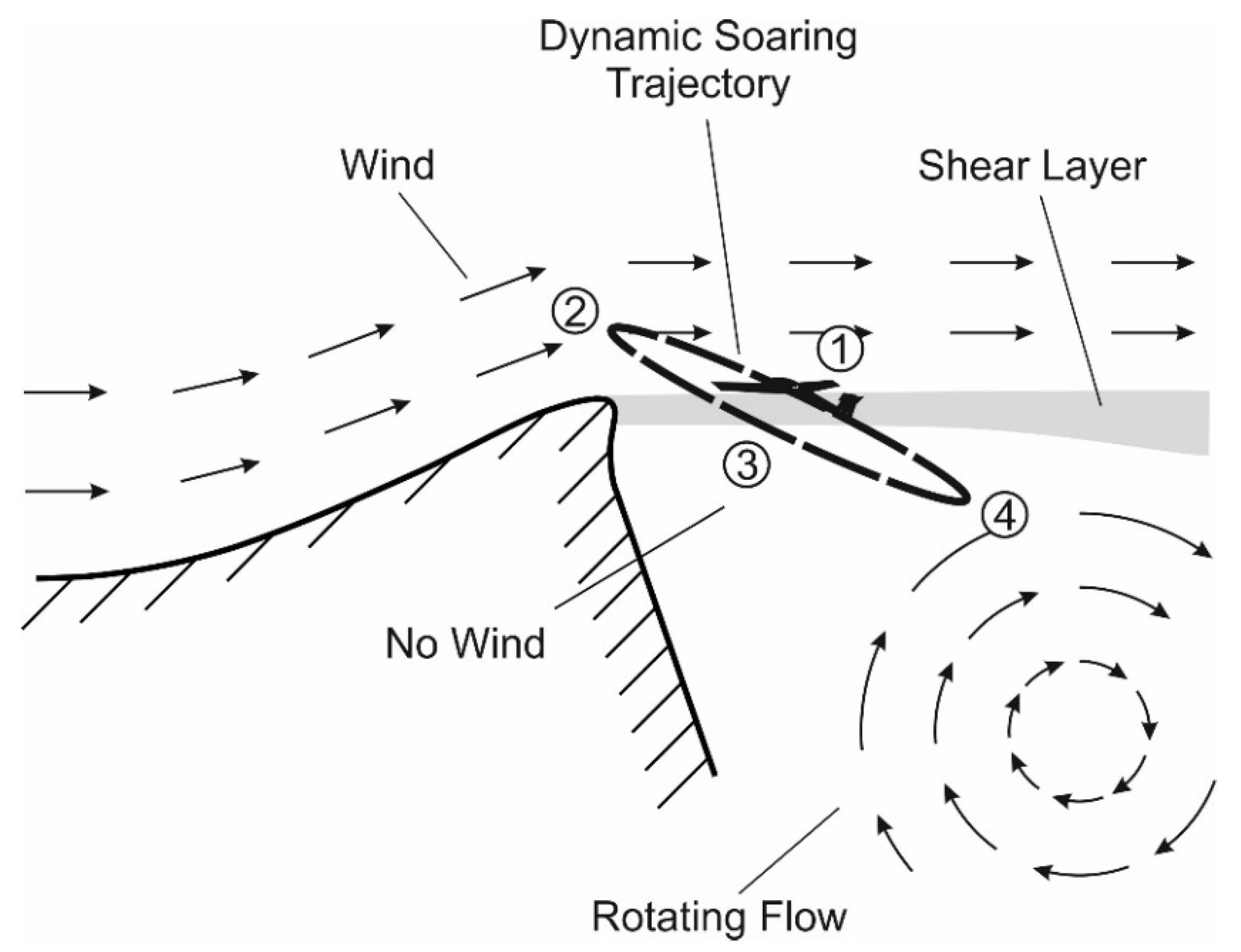
2.1. Modellings of Shear Wind and Vehicle Dynamics

The mode of dynamic soaring appropriate for achieving high speeds is schematically shown in Figure 1. It is possible in wind scenarios where a thin shear layer separates a region of high wind speed from a region of no wind. Such wind scenarios exist in areas leeward of ridges [5]. The high-speed dynamic soaring trajectory consists of a circle-like closed loop where the wind shear layer is traversed upwards in the climb phase and downwards in the descent phase. Characteristically for high-speed dynamic soaring, the inclination of the loop relative to the horizontal is small [16].

Figure 1. High-speed dynamic soaring trajectory at ridge.

The dynamic soaring trajectory comprises four flight phases that are characteristic for this flight mode (indicated by nos. 1 to 4 in Figure 1):

(1)

Windward climb;

(2)

Upper curve in region of high wind speed;

(3)

Leeward descent;

(4)

Lower curve in region of zero or low wind speed.

The wind scenario at the leeward side of the ridge shows features important for high-speed dynamic soaring. There is a shear layer that separates two regions involving different wind characteristics. The region above the layer shows a high wind speed, whereas the region below the layer involves calm air or low wind speeds. Furthermore, the shear layer is thin, implying a small vertical extension.

The model of the wind scenario used in the trajectory optimization of dynamic soaring is presented in Figure 2. The shear layer involves a rapid increase of the wind speed from zero to the value of the free stream wind speed, denoted by $V_{w,ref}$. The transitions to the zero-wind region and to the high wind speed region are modelled as gradual changes in the wind speed.

Figure 2. Modelling of wind scenario at ridge ($V_{w,ref}$: free stream wind speed in region above shear layer).

The motion of aerial vehicles performing high-speed dynamic soaring can be mathematically described using a point-mass dynamics model. Accordingly, the equation of motion in an inertial reference system can be expressed as

$$\begin{gathered} \mathrm{d}{u}_i/\mathrm{d}t=-a_{u1}D/m-a_{u2}L/m \\ \mathrm{d}{v}_i/\mathrm{d}t=-a_{v1}D/m-a_{v2}L/m \\ \mathrm{d}{w}_i/\mathrm{d}t=-a_{w1}D/m-a_{w2}L/m+g \\ \mathrm{d}{x}_i/\mathrm{d}t=u_i \\ \mathrm{d}{y}_i/\mathrm{d}t=v_i \\ \mathrm{d}h/\mathrm{d}t=-w_i \end{gathered}$$

(1)

The coefficients $a_{u1,2}$, $a_{v1,2}$ and $a_{w1,2}$ are factors used for describing relationships regarding the flight path, bank and azimuth angles (${\gamma }_a$, ${\mu }_a$, ${\chi }_a$), yielding

$$\begin{gathered} a_{u1}=\cos {\gamma }_a\cos {\chi }_a \\ {a}_{u2}=\cos {\mu }_a\sin {\gamma }_a\cos {\chi }_a+\sin {\mu }_a\sin {\chi }_a \\ {a}_{v1}=\cos {\gamma }_a\sin {\chi }_a \\ {a}_{v2}=\cos {\mu }_a\sin {\gamma }_a\sin {\chi }_a-\sin {\mu }_a\cos {\chi }_a \\ {a}_{w1}=-\sin {\gamma }_a \\ {a}_{w2}=\cos {\mu }_a\cos {\gamma }_a \end{gathered}$$

(2)

The lift $L$ and the drag $D$ in Equation (1) can be written as

$$\begin{gathered} D=C_D\left(\rho /2\right)V_a^{2}S \\ L=C_L\left(\rho /2\right)V_a^{2}S \end{gathered}$$

(3)

The airspeed, $V_a$, used for describing $L$ and $D$ is relating to the inertial speed components, $u_i$, $v_i$ $w_i$, and the wind speed, $V_w$, according to

$$V_a=\sqrt{{\left(u_i+V_w\right)}^2+v_i^2+w_i^2}$$

(4)

The drag in high-speed dynamic soaring is modelled as being dependent on the lift and the Mach number $Ma$, yielding

$$C_D=C_D(C_L,Ma)$$

(5)

The fact that the dependence of $C_D$ on $Ma$ needs to be accounted for is a unique feature of high-speed dynamic soaring. Usually, gliders soar at a low speed level that relates to the incompressible flight regime so that $C_D$ depends only on $C_L$, but not on $Ma$. By contrast, gliders capable of high-speed dynamic soaring can reach speeds that are in the high subsonic $Ma$ region where compressibility exerts an influence on the aerodynamic characteristics of aerial vehicles (for example, in the case of the above speed record). This holds especially for the drag which shows a significant increase with the Mach number, yielding what is termed compressibility-related drag rise.

The modelling of the drag characteristics for the glider under consideration is graphically addressed in Figure 3 which presents the relationship between $C_D$, $C_L$ and $Ma$. This figure shows that compressibility exerts a strong effect on $C_D$ which progressively increases with $Ma$. Further quantities for modelling the vehicle are the wing reference area $S=0.51 {\mathrm{m}}^2$, the aspect ratio $A=22.5$ and the mass $m=8.5 \mathrm{kg}$. For the described modelling of the vehicle, reference is made to existing vehicles and to experience in this field [6,17,18].

Figure 3. Relationship between drag coefficient, lift coefficient and Mach number.

2.2. Formulation of Optimal Control Problem

The optimization problem is to determine the maximum speed achievable with dynamic soaring. This means to find out the closed-loop dynamic soaring trajectory that shows the maximum speed in the course of the loop. For this purpose, the following performance criterion is specified

$$J\left[\mathit{x}\left(t\right)\right]=V_{inert}\left(t_f\right)$$

(6)

For maximizing $J\left[\mathit{x}\left(t\right)\right]$, the optimal control problem can be formulated as to determine the optimal controls

$${\mathit{u}}^{*}\left(t\right)={[{\widehat{C}}_L^{*}\left(t\right),{\mu }_i^{*}\left(t\right)]}^{\mathrm{T}}$$

(7a)

the optimal states

$${\mathit{x}}^{*}\left(t\right)={[u_i^{*}\left(t\right),v_i^{*}\left(t\right),w_i^{*}\left(t\right),x^{*}\left(t\right),y^{*}\left(t\right),h^{*}\left(t\right)]}^{\mathrm{T}}$$

(7b)

and the associated optimal cycle time $t_{cyc}$, subject to the dynamic system according to Equation (1)

$$\dot{\mathit{x}}\left(t\right)=\mathit{f}\left(\mathit{x}\left(t\right),\mathit{u}\left(t\right)\right)$$

(7c)

to control and state constraints

$$\begin{gathered} C_{L,min}\le C_L\le C_{L,max} \\ h\ge h_{min} \end{gathered}$$

(7d)

and to periodicity boundary conditions

$$\Psi \left(\mathit{x}\right)=\mathit{x}\left(t_{cyc}\right)-\mathit{x}\left(0\right)=\mathbf{0}$$

(7e)

The optimal control problem is solved using the direct optimal control tool FALCON.m [19]. To this end, a full discretization of the optimal control problem on the time grid $\stackrel{-}{\mathit{t}}$ is performed, resulting in the discretized states $\stackrel{-}{\mathit{x}}$ and controls $\stackrel{-}{\mathit{u}}$. The dynamic constraints given by the equations of motion are replaced by a set of defect equations (equality constraints)

$${\mathit{c}}_{\mathit{e}\mathit{q},\mathit{k}}\left(\overline{\mathit{x}},\overline{\mathit{u}}\right)={\stackrel{-}{x}}_{k+1}-{\stackrel{-}{x}}_k-\frac{{\overline{t}}_{k+1}-{\overline{t}}_k}{2}\left[\mathit{f}\left({\stackrel{-}{x}}_{k+1},{\stackrel{-}{u}}_{k+1}\right)+\mathit{f}\left({\stackrel{-}{x}}_k,{\stackrel{-}{u}}_k\right)\right]=\mathbf{0}$$

(8)

at every point on the discretized time grid. These constraints represent a trapezoidal quadrature of the dynamic equations. Furthermore, all path constraints given in Equation (7d), i.e., box constraints on selected control and state variables, are evaluated on this grid, yielding

$${\mathit{c}}_{\mathit{i}\mathit{n}\mathit{e}\mathit{q},\mathit{k}}\left(\overline{\mathit{x}},\overline{\mathit{u}}\right)=\left[\begin{array}{c}{C}_{L,min}-{\overline{C}}_{L,k}\\ {\overline{C}}_{L,k}-C_{L,max }\\ h_{min}-{\overline{h}}_k\end{array}\right]\le \mathbf{0}$$

(9)

for every point ${\overline{t}}_k$ on the discretized time grid. Using the above-mentioned discretized approximations of the objective function, differential equations and constraints contained in the original optimal control problem, the Lagrangian function can be constructed for a nonlinear programming (NLP) problem:

$$\mathcal{L}={\lambda }_0\cdot V_{inert}\left({\overline{t}}_f\right)+{\mathit{\lambda }}_k^{\mathrm{T}}\cdot {\mathit{c}}_{\mathit{e}\mathit{q},\mathit{k}}\left(\overline{\mathit{x}},\overline{\mathit{u}}\right)+{\mathit{\lambda }}_{\mathsf{\Psi }}^{\mathrm{T}}\cdot \Psi \left(\overline{\mathit{x}}\right)+{\mathit{\mu }}_k^{\mathrm{T}}\cdot {\mathit{c}}_{\mathit{i}\mathit{n}\mathit{e}\mathit{q},\mathit{k}}\left(\overline{\mathit{x}},\overline{\mathit{u}}\right)$$

(10)

The optimization software IPOPT [20] is utilized to find the solution of the constructed NLP problem which employs an interior-point method solving for the (Karush–Kuhn–Tucker) first-order optimality conditions

$$\begin{array}{cc}(optimality)\hfill & {\nabla }_{\mathit{z}}\mathcal{L}=\mathbf{0}\end{array}$$

(11a)

$$\begin{array}{cc}(feasibility)\hfill & {\nabla }_{\mathit{\lambda }}\mathcal{L}=\mathbf{0}\end{array}$$

(11b)

$$\begin{array}{cc}(complementarity)\hfill & {\mathit{\mu }}_k^{\mathrm{T}}\cdot {\mathit{c}}_{\mathit{i}\mathit{n}\mathit{e}\mathit{q},\mathit{k}}\left(\overline{\mathit{x}},\overline{\mathit{u}}\right)+\tau =\mathbf{0}\end{array}$$

(11c)

where $\mathit{z}$ represents the primal variables $\left(\overline{\mathit{x}},\overline{\mathit{u}},{\overline{t}}_f\right)$, $\mathit{\lambda }$ and $\mathit{\mu }$ represent dual variables, i.e., the vectors of Lagrange multipliers to equality and inequality constraints, respectively, and $\tau$ is the barrier parameter which is driven to zero by the interior-point optimization software. The corresponding function values, gradient and Hessian matrices are supplied to IPOPT by FALCON.m during every iteration. After calculation of an efficient step in the primal and dual variables, IPOPT returns an updated value of these variables until Equations (11a)–(11c) are satisfied. The solution of the original optimal control problem can be reconstructed from the solution of the NLP.

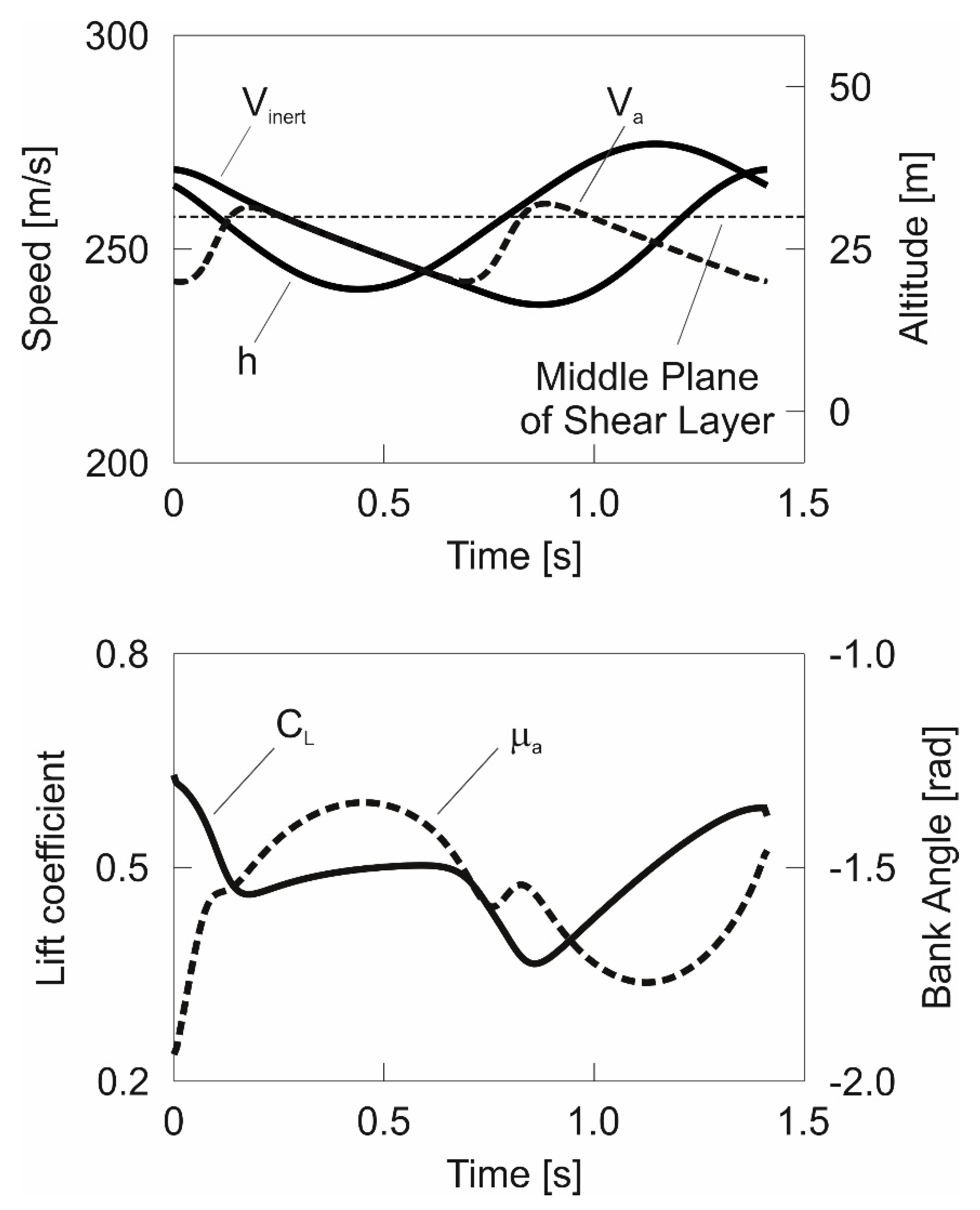
2.3. Results on Trajectory Optimization

A goal of this chapter is to show characteristic features of high-speed dynamic soaring, with emphasis on the features holding in the case of the maximum speed. Another goal is to provide a physical basis that is suitable for developing and validating analytical solutions of high-speed dynamic soaring which will be presented in the next chapter.

Results of the trajectory optimization for dynamic soaring are shown in Figure 4 which provides a perspective view of the closed-loop trajectory of a maximum-speed cycle. The achievable maximum speed determined by the described method of trajectory optimization amounts to $V_{inert,max}=268.6 \mathrm{m}/\mathrm{s}$ (for a given wind speed of $V_{w,ref}=28.5 \mathrm{m}/\mathrm{s}$). The trajectory point where $V_{inert,max}$ occurs is at about the end of the upper curve which is in the upper altitude region where the wind blows. Furthermore, Figure 4 shows how the optimized trajectory relates to the wind and the shear layer.

Figure 4. Dynamic soaring trajectory optimized for maximum speed $V_{inert,max}=268.6 \mathrm{m}/\mathrm{s}$ (Vehicle modelling data used here and in the following are the same as in the chapter “Trajectory Optimization”).

In Figure 5, top and side views are presented for the optimized trajectory. The side view in terms of a projection on the x_i-h plane shows that this involves two lines which are nearly straight and close to each other. Thus, the trajectory can be seen as being virtually in a plane. Furthermore, the inclination of the trajectory is small. The top view in terms of a projection on the x_i-y_i plane shows that this yields a circular-like shape. That feature and the small inclination suggest that the circular characteristic also holds for the trajectory itself. The described trajectory characteristics are part of the basis of a dynamic soaring model that is suitable for developing analytical solutions in the following chapter.

Figure 5. Side and top views of dynamic soaring trajectory optimized for maximum speed $V_{inert,max}=268.6 \mathrm{m}/\mathrm{s}$.

The time histories of the speeds, $V_{inert}$ and $V_a$, and the altitude,$h$, are presented in Figure 6. The $V_{inert}$ time history is plotted such that the maximum speed, $V_{inert,max}=268.6 \mathrm{m}/\mathrm{s}$, occurs at the beginning of the cycle and, because of periodicity reasons, at the end. The altitude shows an oscillation around the middle of the shear layer. The altitude at which $V_{inert,max}$ is reached is above the middle plane of the shear layer, implying that it is not at the lowest point of the trajectory but well above. With reference to Figure 2, the altitude time history shows that the top of the trajectory is above the shear layer and the bottom of the trajectory is below the shear layer. The airspeed $V_a$ the highest value of which is smaller than that of $V_{inert}$ features two oscillations which are rather similar.

Figure 6. Speeds, $V_{inert}$ and $V_a$, altitude,$h$, lift coefficient, $C_L$, and bank angle, ${\mu }_a$, during dynamic soaring cycle optimized for maximum speed $V_{inert,max}=268.6 \mathrm{m}/\mathrm{s}$.

Furthermore, the controls which are the lift coefficient, $C_L$, and the bank angle, ${\mu }_a$, are presented in Figure 6. The lift coefficient features an oscillatory behavior around $C_L=0.5$, with the lowest values occurring in the windward climb phase. The bank angle involves an oscillatory behavior around −1.5 where the banked attitude is smaller during the lower curve when compared with the upper curve.

The energy characteristics of the optimized trajectory are presented in Figure 7 which shows the energy gain from the wind and the energy loss due to the drag. The line denoted by energy gain from wind shows that the energy gain is achieved in the second half of the cycle. This cycle half is relating to the upper curve, as shown in Figure 4. The upper curve, together with the high wind speed in that altitude region, is essential for a large energy gain [21]. In the first half of the cycle, there is no energy gain because the vehicle is in a zone of zero wind. Other than the energy gain, the energy loss due to the drag takes place throughout the entire cycle. The energy loss shows a continuous increase which appears as a nearly straight line. At the end of the cycle, the energy gain from the wind and the energy loss due to the drag agree, to the effect that there is an energetically balanced flight condition. The described characteristics concerning the energy gain and the energy loss will be used in developing the dynamic soaring model that is suitable for deriving analytical solutions in the following chapter.

Figure 7. Energy gain from wind and energy loss due to drag during dynamic soaring cycle optimized for maximum speed $V_{inert,max}=268.6 \mathrm{m}/\mathrm{s}$.

For controlling the drag as the cause of the energy loss and for minimizing related detrimental effects, the relationship between drag and lift as a measure for the aerodynamic efficiency is important. Appropriate quantities for describing this are the actual lift-to-drag ratio, $C_L/C_D$, and the maximally possible lift-to-drag ratio, ${(C_L/C_D)}_{max}$. The time histories of these quantities are plotted in Figure 8. Comparing the two curves, it turns out that they are close to each other and overlap in parts. As a result, the flight is performed close to or at the highest aerodynamic efficiency in terms of the maximum lift-to-drag ratio, ${(C_L/C_D)}_{max}$. This characteristic will also be used in developing the dynamic soaring model that is suitable for deriving analytical solutions in the following chapter.

Figure 8. Actual lift-to-drag ratio, $C_L/C_D$, and maximum lift-to-drag ratio, ${(C_L/C_D)}_{max}$, during dynamic soaring cycle optimized for maximum speed $V_{inert,max}=268.6 \mathrm{m}/\mathrm{s}$.

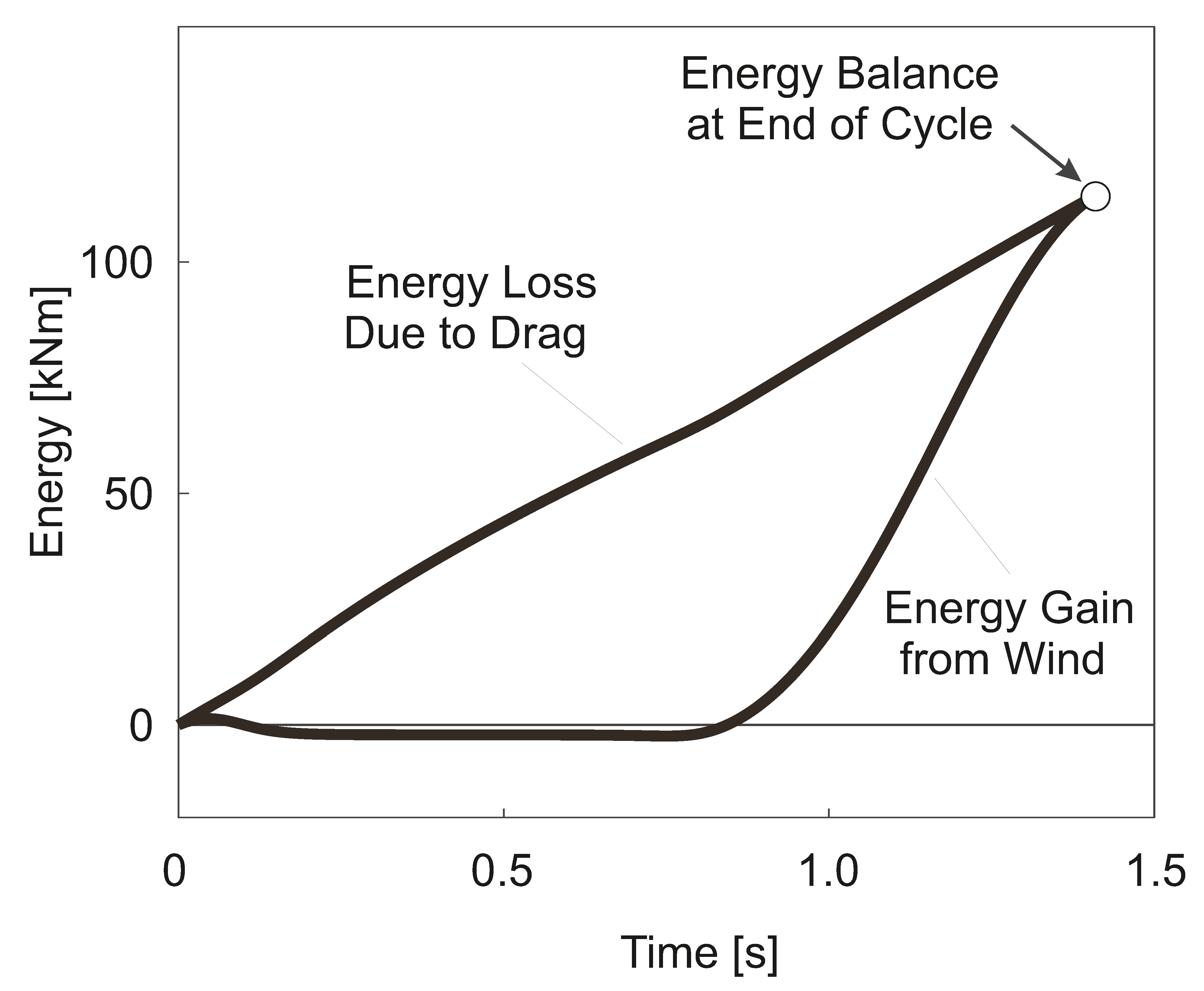
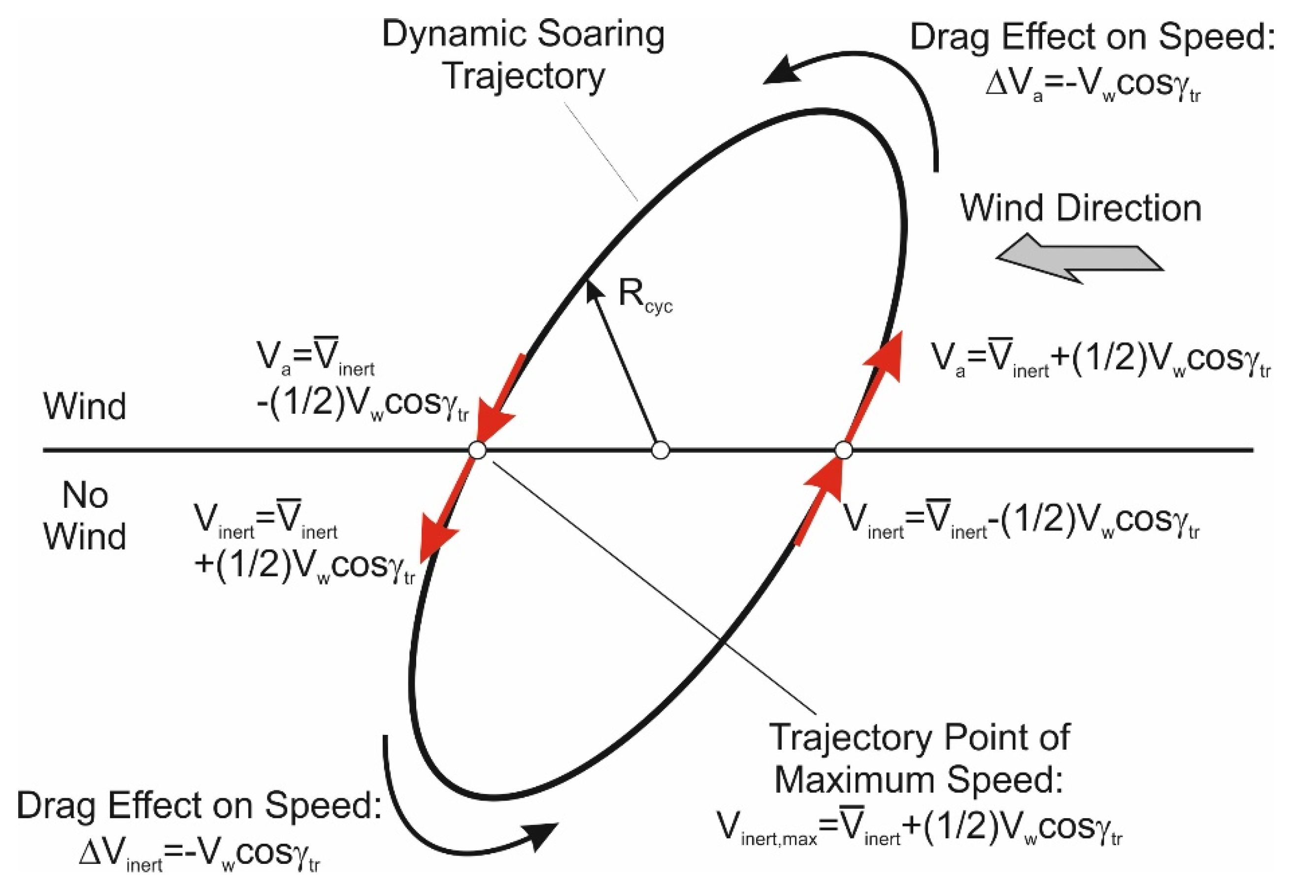
3. Energy Based Model of High-Speed Dynamic Soaring

To develop an energy-based flight mechanics model appropriate for deriving analytical solutions of high-speed dynamic soaring, assumptions about the trajectory and speeds are made. These assumptions are related to the results on trajectory optimization that are presented and discussed in the previous chapter.

As a starting point of developing an appropriate flight mechanics model, an oblique view of a dynamic soaring loop is presented in Figure 9. It is assumed in accordance with Figure 5 that the dynamic soaring loop is circular and the inclination is small. Furthermore, it is presupposed that the shear layer thickness is infinitesimally small. Another modeling aspect is that the dynamic soaring loop can be subdivided into two sections of which one is in the upper part of the loop where the wind is blowing and the other is in the lower loop part where the wind is zero.

Figure 9. Oblique view of a dynamic soaring loop (The trajectory inclination relative to the horizontal is shown overlarge for a clear representation of the pictorial elements).

Each time the shear layer is traversed, there is an approximate speed increase of $\left(1/2\right)V_w\cos {\gamma }_{tr}$. This yields for the airspeed in the windward climb after the transition point

$$V_a={\overline{V}}_{inert}+\frac{1}{2}{V}_w\cos {\gamma }_{tr}$$

(12)

and for the inertial speed in the leeward descent after the transition point

$$V_{inert}={\overline{V}}_{inert}+\frac{1}{2}{V}_w\cos {\gamma }_{tr}$$

(13)

where ${\overline{V}}_{inert}$is the average inertial speed of the loop and ${\gamma }_{tr}$ is the flight path angle at the transition point. These speed relations, together with the speed relations before the transition points (as indicated in Figure 9), relate to the periodicity characteristic of the loop cycle. This includes the effect of drag on the speed in the upper and lower parts of the loop, also indicated in Figure 9, yielding for the speed decreases $\Delta V_a=-\left(1/2\right)V_w\cos {\gamma }_{tr}$ and $\Delta V_{inert}=-\left(1/2\right)V_w\cos {\gamma }_{tr}$, respectively.

In the speed relations presented in Figure 9, the order of magnitude in the relationships between the speeds $V_{inert}$, $V_a$ and $V_w$ is accounted for. These relationships are graphically addressed in Figure 10, where speed vector triangles at two distinct points are presented; one refers to the windward climb and the other to the upper curve around the top of the trajectory. These results are from the trajectory optimization treatment performed in the previous chapter. The speed vector triangles in Figure 10 show that

$$\begin{gathered} V_w\ll V_{inert} \\ {V}_w\ll V_a \end{gathered}$$

(14)

Thus, the following relation applies in the wind region

$$V_a\approx V_{inert}$$

(15a)

In the zero-wind region, both speeds are equal, yielding

$$V_a=V_{inert}$$

(15b)

The described order of magnitude regarding $V_{inert}$, $V_a$ and $V_w$ can be considered as characteristic for high-speed dynamic soaring.

Figure 10. Speed vector triangles in windward climb (flight phase 1) and in upper curve (flight phase 2).

The energy gain from the wind is achieved in the upper section of the loop where the wind is blowing, as shown in Figure 7. This leads to an energy increase given by the kinetic energy increase between the two transition points which are at the same altitude, yielding

$$E_g=\frac{m}{2}\left[{\left({\overline{V}}_{inert}+\frac{1}{2}{V}_w\cos {\gamma }_{tr}\right)}^2-{\left({\overline{V}}_{inert}-\frac{1}{2}{V}_w\cos {\gamma }_{tr}\right)}^2\right]=m{\overline{V}}_{inert}{V}_w\cos {\gamma }_{tr}$$

(16)

The energy increase $E_g$ which is the net energy increase accounting for the drag-related loss in the upper loop section is required for balancing the work done by the drag in the lower loop section.

The drag work in the lower loop section can be expressed as

$$W_D=-\underset{t_1}{\overset{t_{cyc}}{{\displaystyle \int }}}D{V}_{inert}\mathrm{d}t$$

(17)

where $t_1$ refers to the transition from the wind region to the zero-wind region.

For expanding the drag work expression, the relation between the drag and the lift in curved flight is accounted for, yielding

$$D=\frac{C_D}{C_L}L=\frac{C_D}{C_L}nmg$$

(18)

It is assumed for the problem under consideration that the $C_D/C_L$ ratio and the load factor $n$ are constant. Thus, the following approximate result of the drag work can be derived from Equation (17)

$$W_D=-\frac{C_D}{C_L}nmgs$$

(19)

where

$$s=\pi R_{cyc}$$

(20)

is the length of the lower loop section.

Further to expanding the drag work expression, the relation between $n$, $R_{cyc}$ and ${\overline{V}}_{inert}$ in curved flight is introduced, yielding for sufficiently small flight path angles

$$n=\sqrt{1+{\left(\frac{{\overline{V}}_{inert}^2}{R_{cyc}g}\right)}^2}$$

(21a)

Since the load factor in high-speed dynamic soaring is of the order of $n=100$ [5,6,16], Equation (21a) can be replaced by

$$n=\frac{{\overline{V}}_{inert}^2}{R_{cyc}g}$$

(21b)

Thus, the drag work can be expressed as

$$W_D=-\pi \frac{C_D}{C_L}m{\overline{V}}_{inert}^2$$

(22)

The balance of the drag work and the energy gain is given by

$$E_g+W_D=0$$

(23)

Using this relation and Equation (22), the average inertial speed is obtained as

$${\overline{V}}_{inert}=\frac{1}{\pi }\frac{C_L}{C_D}{V}_w\cos {\gamma }_{tr}$$

(24)

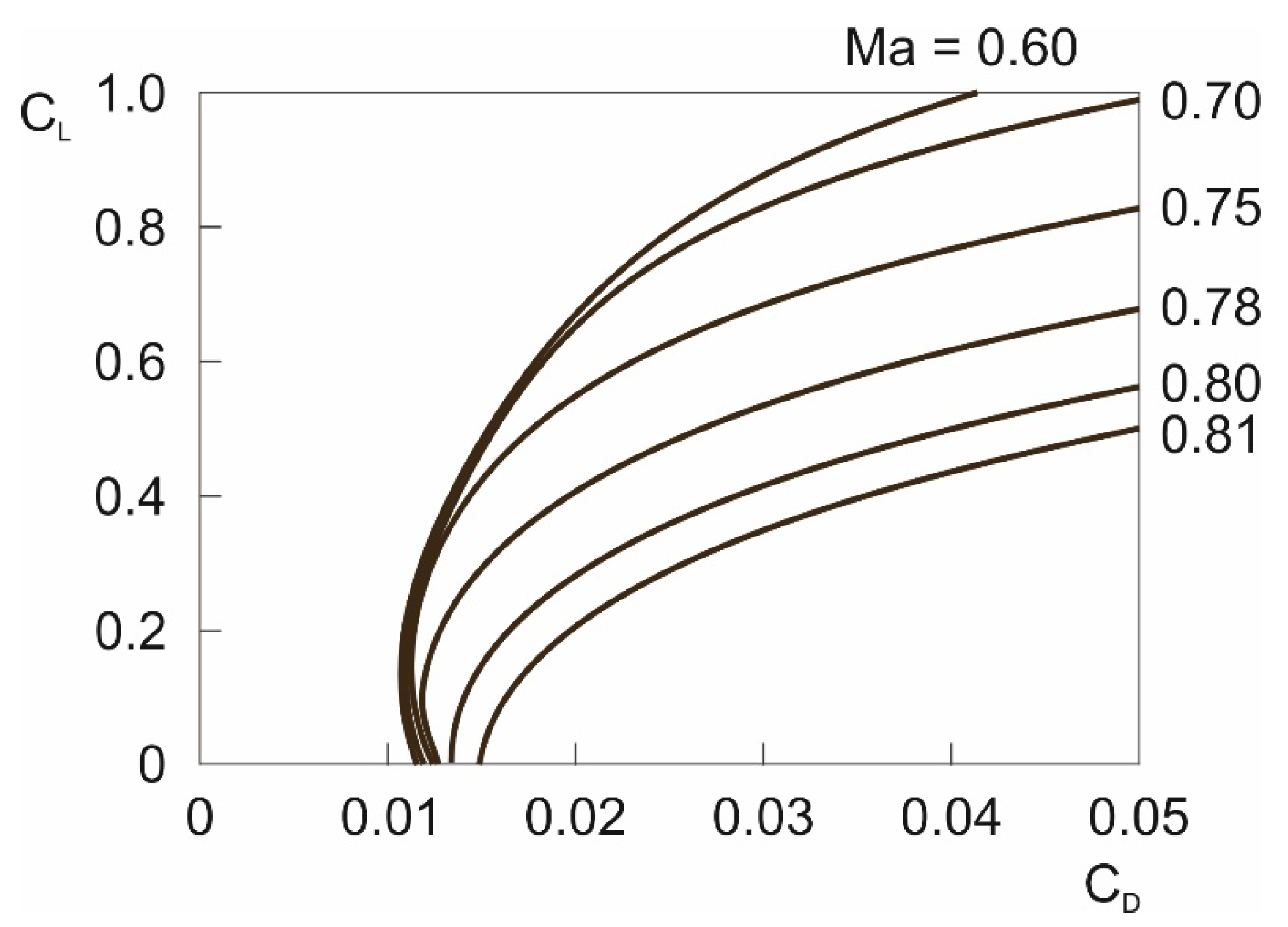
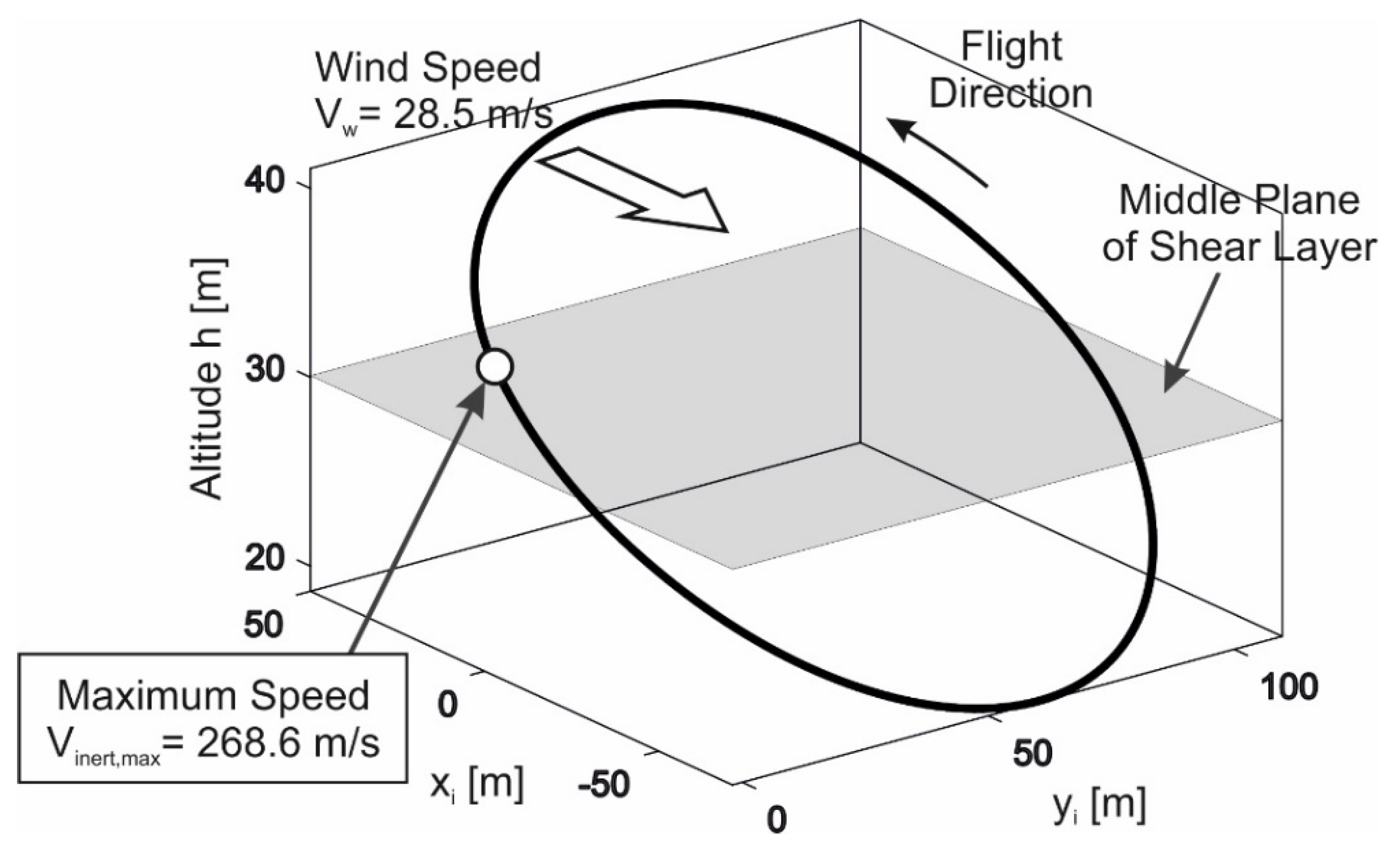
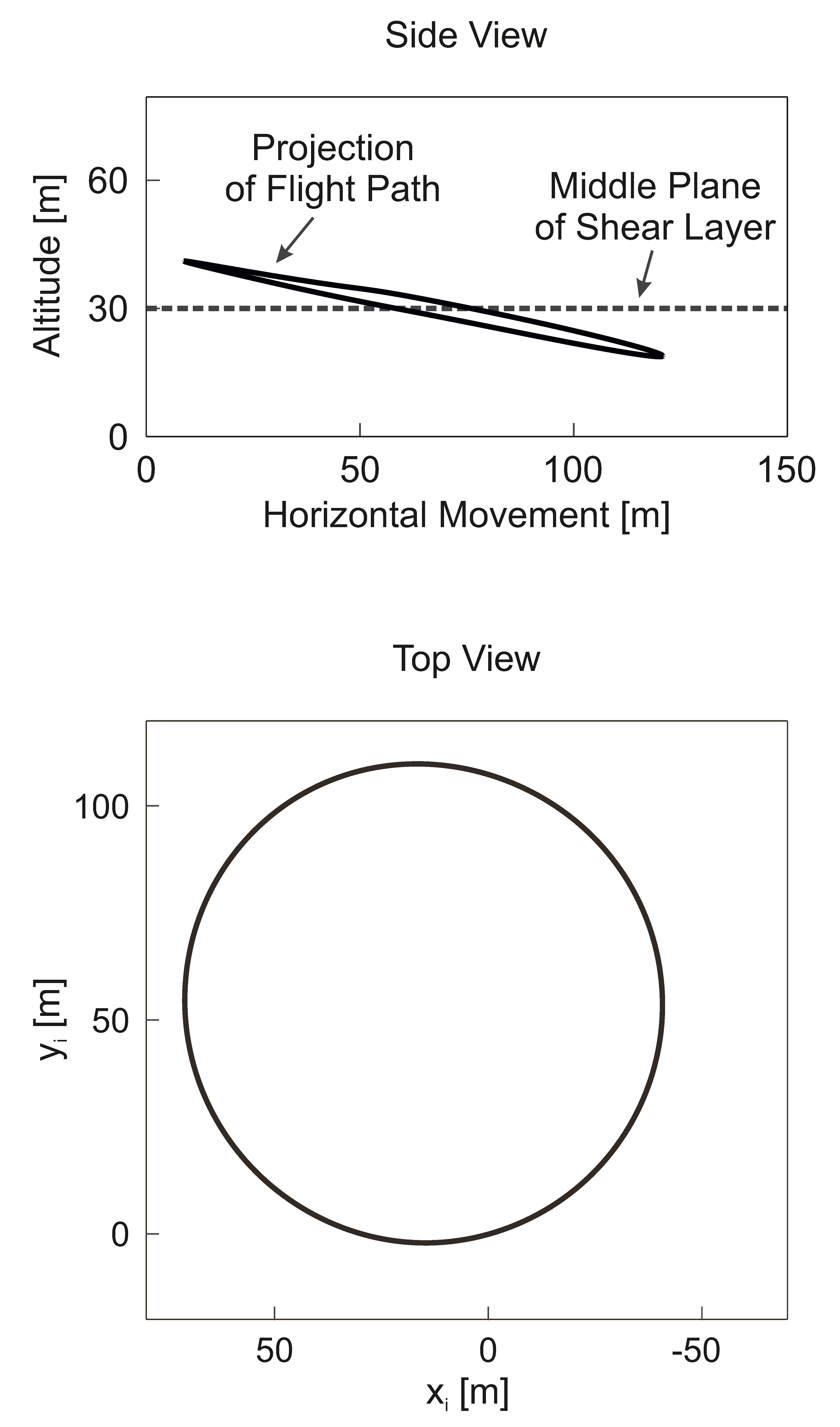
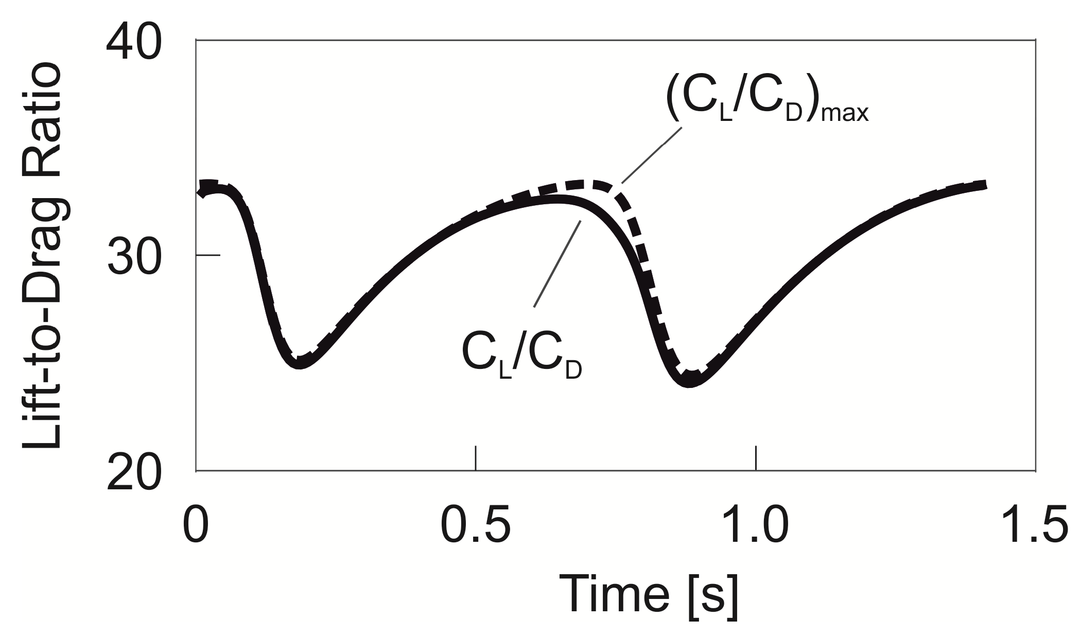
4. Maximum Speed Performance

The results presented in Figure 6 and Figure 9 show that the highest speed in the dynamic soaring loop—which is larger than ${\overline{V}}_{inert}$—occurs in the leeward descent at the transition point, as given by Equation (13). Accounting for this, and the fact that average inertial speed ${\overline{V}}_{inert}$ shows its greatest value at the maximum lift-to-drag ratio ${(C_L/C_D)}_{max}$ according to Equation (24), the following result on the maximum speed is obtained

$$V_{inert,max}=\left[\frac{1}{2}+\frac{1}{\pi }{\left(\frac{C_L}{C_D}\right)}_{max}\right]V_w\cos {\gamma }_{tr}$$

(25)

Assuming ${\gamma }_{tr}\ll 1$ in accordance with the results of the trajectory optimization on the smallness of the trajectory inclination (Figure 5), the relation of the maximum speed can be simplified to yield

$$V_{inert,max}=\left[\frac{1}{2}+\frac{1}{\pi }{\left(\frac{C_L}{C_D}\right)}_{max}\right]V_w$$

(26)

This relation provides an analytical solution for the maximum speed. Thus, a main goal of the treatment of high-speed dynamic soaring is achieved, and results of generally valid nature can be obtained.

Further to the relation given in Equation (26), the key factors for the maximum speed are identified, yielding

(1)

Wind speed, $V_w$;

(2)

Maximum lift-to-drag ratio in terms of ${(C_L/C_D)}_{max}$.

This means that there is no other factor that has an influence. For instance, the size or the mass of the vehicle or the altitude which usually have significant effects on the flight performance of aerial vehicles are without influence.

Moreover, the influence of the key factors on the achievable maximum speed is determined. The effect of the key factors on the achievable maximum speed is such that each of them yields a linear influence on $V_{inert,max}$. The overall effect is due to the product of both key factors.

The relationship between $V_{inert,max}$ and the key factors $V_w$ and ${(C_L/C_D)}_{max}$ is graphically addressed in Figure 11. The objective here is to show the validity of the energy-based model and the related analytical solution. Two $V_{inert,max}$curves are presented: one is the outcome of the analytical solution described by Equation (26), and the other is the outcome of the trajectory optimization using the vehicle dynamics model of the previous chapter. Basically, the two $V_{inert,max}$curves are close to each other and overlap in parts, with the result that both solutions virtually agree. This can be seen as a validation of the energy-based model. In the following sections, more details on the validity issue are provided.

Figure 11. Maximum speed $V_{inert,max}$.

Examining the curve characteristics in Figure 11, the left part of the $V_{inert,max}$ curve shows a comparatively large and constant gradient, whereas the gradient in the right part is reduced. Relating the behavior of the $V_{inert,max}$ gradient to the Mach number $Ma$ indicated on the ordinate shows that the change in the gradient starts in a zone where compressibility becomes effective. This is the zone where compressibility begins to become effective for the aerodynamic characteristics of the vehicle. Thus, the left part of the $V_{inert,max}$ curve can be related to the incompressible $Ma$ region, whereas the right part to the compressible one.

The differences in the left and right curve parts are due to the effect of compressibility on the maximum lift-to-drag ratio ${(C_L/C_D)}_{max}$ as one of the key factors for $V_{inert,max}$, Equation (26). Evidence of the compressibility effect is provided by Figure 12 which presents results from an examination of the drag polar plotted in Figure 3 with regard to ${(C_L/C_D)}_{max}$. In the incompressible $Ma$ region, ${(C_L/C_D)}_{max}$ is constant and shows the highest level. In the Mach number zone where compressibility becomes effective, ${(C_L/C_D)}_{max}$ begins to decrease to become continually smaller with $Ma$ in the compressible $Ma$ region.

Figure 12. Maximum lift-to-drag ratio ${(C_L/C_D)}_{max}$ dependent on the Mach number $Ma$ (relating to drag polar presented in Figure 3).

Returning to Figure 11 and examining the $V_{inert,max}$ characteristics with due regard to the described findings on ${(C_L/C_D)}_{max}$, it becomes clear that these characteristics are the result of the ${(C_L/C_D)}_{max}$ properties. This explains why there are two curve parts showing distinct differences, caused by corresponding differences in ${(C_L/C_D)}_{max}$. Concerning the left curve part, the fact that the gradient is constant and large is due to the constancy and largeness of ${(C_L/C_D)}_{max}$. In the right curve part, the gradient is reduced. This is caused by the decrease of ${(C_L/C_D)}_{max}$ in the compressible $Ma$ region.

The relationship between $V_{inert,max}$ and the key factors $V_w$ and ${(C_L/C_D)}_{max}$ is rather simple in the incompressible $Ma$ region because of the constancy in ${(C_L/C_D)}_{max}$. In the compressible $Ma$ region, this relationship is more complex. Nevertheless, the analytical solution achieved with the energy-based model and the solution obtained with the vehicle dynamics model of the previous chapter agree here too. This fact notably provides evidence for the validity of the energy-based model.

5. Further Issues Concerning High-Speed Dynamic Soaring

The key factors $V_w$ and ${(C_L/C_D)}_{max}$ dealt with above are decisive for the maximum speed performance in terms of $V_{inert,max}$. There are further significant topics of high-speed dynamic soaring where other aspects not related to the speed performance are involved. This concerns issues such as controllability of the vehicle at extremely high speeds or flyability in case of very short cycle periods, high loads acting on the vehicle, required air space and altitude related effects. For these issues, the following quantities can be regarded as representative and relevant:

-

cycle time $t_{cyc}$

-

load factor $n$

-

trajectory extension and loop radius $R_{cyc}$

-

altitude $h$

5.1. Cycle Time $t_{cyc}$

The cycle time, $t_{cyc}$, plays a significant role in high-speed dynamic soaring. This relates to cases of very small $t_{cyc}$ values which cause difficulties in flying and controlling the vehicle. Small $t_{cyc}$ values are a characteristic feature of high-speed dynamic soaring [5,6,17]. There are $t_{cyc}$ values of such small a magnitude in high-speed dynamic soaring that they are regarded critical. This is because cycle times of around 2 s, or smaller, are considered as difficult to fly in practice.

The cycle time is basically given by the relation

$$t_{cyc}=\frac{2\pi R_{cyc}}{{\overline{V}}_{inert}}$$

(27)

For expanding this expression, reference is made to the load factor relation in curved flight

$$n=\frac{C_L\left(\rho /2\right){\overline{V}}_{inert}^{2}S}{mg}$$

(28)

Using this relation and accounting for Equation (21b), the cycle time dependent on the average speed ${\overline{V}}_{inert}$ and the lift coefficient $C_L$ can be expressed as

$$t_{cyc}=2\pi \frac{m}{C_L\left(\rho /2\right)S{\overline{V}}_{inert}}$$

(29)

The optimal lift coefficient for achieving the maximum speed $V_{inert,max}$ is the one associated with ${(C_L/C_D)}_{max}$. Denoting this lift coefficient by $C_L^{*}$, and referring to Equations (24) and (26), the following result for the optimal cycle time dependent on the maximum speed $V_{inert,max}$ is obtained, yielding

$$t_{cyc}=2\pi \frac{m}{C_L^{*}\left(\rho /2\right)S\left(V_{inert,max}-V_w/2\right)}$$

(30)

The relationship between $t_{cyc}$ and $V_{inert,max}$ is graphically addressed in Figure 13. There is a decrease of $t_{cyc}$ with $V_{inert,max}$ until a value of about $V_{inert,max}=260 \mathrm{m}/\mathrm{s}$is reached. Thereafter, an increase of $t_{cyc}$ occurs. With reference to the $V_{inert,max}=260 \mathrm{m}/\mathrm{s}$ value and Figure 11, it can be concluded that the $V_{inert,max}$ region involving the $t_{cyc}$ decrease relates to the incompressible regime, while the $V_{inert,max}$ region showing the $t_{cyc}$ increase is associated with the compressible regime.

Figure 13. Optimal cycle time $t_{cyc}$ dependent on $V_{inert,max}$.

The reason why $t_{cyc}$ shows an increase in the upper $V_{inert,max}$ region (rather than a continuation of the decrease) is due to $C_L^{*}$ and its dependence on the Mach number $Ma$. The relationship between $C_L^{*}$ and $Ma$ is shown in Figure 14, based on an examination of the drag polar presented in Figure 3 with regard to ${(C_L/C_D)}_{max}$ and $C_L^{*}$, respectively. This relationship is such that $C_L^{*}$ is constant in the incompressible $Ma$ region whereas there is a decrease of $C_L^{*}$ in the compressible $Ma$ region. That decrease of $C_L^{*}$ is so strong that it outweighs the opposing effect of the increase of $V_{inert,max}$ in the denominator of Equation (30), with the result that $t_{cyc}$ is increased.

Figure 14. Optimal lift coefficient ${\mathrm{C}}_{\mathrm{L}}^{*}$ dependent on Mach number $Ma$.

The results presented in Figure 13 show that the decrease of $t_{cyc}$ is stopped and even reversed, occurring in the upper $V_{inert,max}$ range where the $t_{cyc}$ level is lowest. This can be considered a favorable effect, especially if $t_{cyc}$ is very small and of a magnitude regarded as critical.

5.2. Load Factor $n$

The loops performed in high-speed dynamic soaring involve rapid turning at a large speed. The centrifugal force associated with this flight condition leads to high loads acting on the vehicle, yielding load factors of an order of magnitude as large as 100 [5]. Accordingly, large loads are typical for high-speed dynamic soaring [6].

The load factor, dependent on the average speed ${\overline{V}}_{inert}$ and the lift coefficient $C_L$, is given by Equation (28). The lift coefficient for achieving the maximum speed $V_{inert,max}$ is $C_L^{*}$. Referring to Equations (24) and (26), the following result for the load factor flying at the maximum speed $V_{inert,max}$ is obtained, yielding

$$n=\frac{C_L^{*}\left(\rho /2\right)S}{mg}{\left(V_{inert,max}-V_w/2\right)}^2$$

(31)

The load factor $n$ dependent on $V_{inert,max}$ is presented in Figure 15. According to Equation (31), there is a quadratic increase of $n$ with $V_{inert,max}$ until a value of about $V_{inert,max}=260 \mathrm{m}/\mathrm{s}$is reached. Thereafter, $n$ shows a decrease. The two $V_{inert,max}$ regions, one showing a decrease and the other an increase of $n$, relate to the incompressible and compressible regimes, respectively. The reason for these differences in the $n$ effects is again due to $C_L^{*}$ and its dependence on the Mach number $Ma$, as shown in Figure 14.

Figure 15. Load factor $n$ dependent on $V_{inert,max}$.

5.3. Trajectory Extensions and Loop Radius $R_{cyc}$

High-speed dynamic soaring involves a closed-loop trajectory showing extensions in the longitudinal and lateral directions. A question is whether or not the extensions of the trajectory depend on the maximum speed $V_{inert,max}$. In case that the trajectory extensions are not independent of $V_{inert,max}$, the trajectory has to be adapted for a change in $V_{inert,max}$. This implies that a change in the trajectory extensions is necessary if $V_w$ changes, because $V_{inert,max}$ is dependent on the wind speed $V_w$ (Figure 11). The loop radius is considered a quantity that can be used to describe the relationship between the extensions of the trajectory and $V_{inert,max}$.

With reference to Equations (21b) and (28), the radius of the loop in high-speed dynamic soaring can be expressed as

$$R_{cyc}=\frac{m}{C_L\left(\rho /2\right)S}$$

(32)

Since the lift coefficient for achieving the maximum speed $V_{inert,max}$ is $C_L^{*}$, the relation for the optimal loop radius is obtained as

$$R_{cyc}=\frac{m}{C_L^{*}\left(\rho /2\right)S}$$

(33)

This relation shows that there is no direct dependence of $R_{cyc}$ on $V_{inert,max}$ or $V_w$. The only effect is due to $C_L^{*}$ in case that $C_L^{*}$ depends on the Mach number $Ma$ (Figure 14). Thus, $R_{cyc}$ is constant in the incompressible $Ma$ region since $C_L^{*}$ is constant here. In the compressible $Ma$ region, $R_{cyc}$ shows changes inversely proportional to $C_L^{*}$, to the effect that $R_{cyc}$ increases with $V_{inert,max}$ because of the decrease of $C_L^{*}$ with an increase of $Ma$.

The dependence of $R_{cyc}$ on $V_{inert,max}$ is presented in Figure 16. The loop radius is constant up to a $V_{inert,max}$ value where compressibility becomes effective. Thereafter, a continual increase of $R_{cyc}$ takes place. The results from the trajectory optimization (Chapter 2) are determined using the average of the greatest extensions in the x_i nd y_i directions.

Figure 16. Optimal loop radius $R_{cyc}$ dependent on $V_{inert,max}$.

5.4. Effects of Altitude $h$

There are different aspects concerning the effects of the altitude on high-speed dynamic soaring. Basically, these effects are due to the dependencies of the air density and the speed of sound on the altitude $h$, i.e., $\rho =\rho \left(h\right)$ and $a=a\left(h\right)$. This relates to all quantities treated above, including $V_{inert,max}$ as well as $t_{cyc}$, $n$ and $R_{cyc}.$

A main aspect is how the maximum speed performance in terms of $V_{inert,max}$ is influenced by the altitude. The relation of $V_{inert,max}$ given in Equation (26) shows that there is no term involving an explicit dependence on the altitude $h$. However, there is an altitude effect which is associated with the dependence of ${\left(C_L/C_D\right)}_{max}$ on $Ma$ (Figure 12). This refers to the following relation between $Ma$ and $h$:

$$Ma=V_a/a\left(h\right)$$

(34)

Since this is relevant only if compressibility becomes effective for ${\left(C_L/C_D\right)}_{max}$, it can be distinguished between the incompressible and the compressible $Ma$ regions regarding the effect of $h$ on $V_{inert,max}$. In the incompressible $Ma$ region, where ${\left(C_L/C_D\right)}_{max}$ is constant, there is no altitude effect so that $V_{inert,max}$ is independent of $h$. In the compressible $Ma$ region, an altitude effect exists due to the dependence of ${\left(C_L/C_D\right)}_{max}$ on $Ma$. As the speed of sound, $a$, shows comparatively little changes with $h$ (e.g., 3% between 0 and 3000 m), the relation for $V_{inert,max},$ Equation (26), together with the dependence of ${\left(C_L/C_D\right)}_{max}$ on $Ma$, Figure 12, suggests that the effect of $h$ on $V_{inert,max}$ is mall.

The described relationship between $V_{inert,max}$ and $h$ is graphically addressed in Figure 17 which shows $V_{inert,max}$ dependent on $V_w$ for $h=0$ and $h=3000 \mathrm{m}$, thus including $V_{inert,max}$ for the altitude range between these values. The left part of the $V_{inert,max}$ curve which is associated with the incompressible Ma region holds for both $h$ values, whereas the right curve part associated with the compressible Ma region shows a small reduction at $h=3000 \mathrm{m}$ compared to $h=0$.

Figure 17. Effect of altitude $h$ on maximum speed $V_{inert,max}$. Upper curve in each of solid and dotted lines relates to $h=0 \mathrm{m}$, and lower curve in each of solid and dotted lines relates to $h=3000 \mathrm{m}$ (atmosphere data from [22]).

In regard to the quantities $t_{cyc}$, $n$ and $R_{cyc}$, there are effects of the altitude $h$ associated with the air density $\rho$ and the speed of sound $a$. The expressions given in Equations (30), (31) and (33) show that the effect of $\rho$ manifests explicitly in a dependence that is linear in $\rho$ or inversely proportional to $\rho$. The effect of $a$ relates to the dependencies of $C_L^{*}$ and ${\left(C_L/C_D\right)}_{max}$ on $Ma$ (Figure 12 and Figure 14) and the relation between $Ma$ and $a\left(h\right)$ as given by Equation (34). Accordingly, it can be distinguished between the incompressible and the compressible $Ma$ regions regarding the effects of $h$. In the incompressible $Ma$ region, there is no altitude effect on $C_L^{*}$ and ${\left(C_L/C_D\right)}_{max}$ so that each of $t_{cyc}$, $n$ and $R_{cyc}$ is only dependent on $\rho$as described by Equations (30), (31) and (33). In the compressible $Ma$ region, an additional altitude effect exists due to the dependencies of $C_L^{*}$ and ${\left(C_L/C_D\right)}_{max}$ on $Ma$.

Concerning the optimal cycle time, the effect of the altitude is presented in Figure 18 which shows $t_{cyc}$for two altitude cases. Basically, $t_{cyc}$increases with an increase of $h$. This is a favorable effect, especially in the case of very small $t_{cyc}$ values. Furthermore, the difference between the two $t_{cyc}$ curves is significant. For the incompressible $Ma$ region in Figure 18, where $t_{cyc}$ is only dependent on $\rho$, the following result on the relation between $t_{cyc}$ and $h$ can be obtained from Equation (30) to yield

$$t_{cyc}=\frac{{\rho }_0}{\rho \left(h\right)}{t}_{cyc,0}$$

(35)

with ${\rho }_0$ and $t_{cyc,0}$ denoting the values at $h=0$.

Figure 18. Effect of altitude $h$ on optimal cycle time $t_{cyc}$.

The effect of the altitude on the load factor is presented in Figure 19 which shows $n$for two altitude cases. As a basic result, $n$decreases with the increase of $h$. This can be considered a favorable effect as the load on the vehicle is reduced. For the incompressible Ma region, where $n$ depends only on $\rho$, the relation between $n$ and $h$ can be expressed as

$$n=\frac{\rho \left(h\right)}{{\rho }_0}{n}_0$$

(36)

where $n_0$ denotes the load factor at $h=0$.

Figure 19. Effect of altitude $h$ on load factor $n$.

The effect of altitude on the optimal loop radius $R_{cyc}$is presented in Figure 20, where $R_{cyc}$ is plotted for the two altitude cases under consideration. Basically, $R_{cyc}$ increases with the altitude $h$ and the shape of the $R_{cyc}$ curve involving a constant part for a large $V_{inert,max}$ range is retained. The constant part of $R_{cyc}$ relates to the incompressible $Ma$ region, where $R_{cyc}$ is dependent only on $\rho$. Here, the effect of the altitude can be expressed as

$$R_{cyc}=\frac{{\rho }_0}{\rho \left(h\right)}{R}_{cyc,0}$$

(37)

where $R_{cyc,0}$ denotes the optimal loop radius at $h=0$. In the compressible Mach number region, there are additional altitude effects due to the dependencies of $C_L^{*}$ and ${\left(C_L/C_D\right)}_{max}$ on $Ma$.

Figure 20. Effect of altitude $h$ on optimal loop radius $R_{cyc}$.

5.5. Final Remark on Validity of Energy Based Model and Related Analytical Solutions

Concerning the results presented in the current Chapter 5, the goal here is also to show the validity of the derived analytical solutions. The analytical solutions using the energy-based model and the results obtained with the trajectory optimization using the vehicle dynamics model of Chapter 2 “Trajectory Optimization” virtually agree. This holds for all topics of high-speed dynamic soaring dealt with, including the maximum inertial speed $V_{inert,max}$ as the most important quantity, the cycle time $t_{cyc}$, the load factor $n$, the loop radius $R_{cyc}$ and the effects of the altitude. This is considered a validation of the energy-based model and the related analytical solutions of dynamic soaring.

6. Conclusions

Trajectory optimization is used as a means to determine the maximum speed achievable in high-speed dynamic soaring and to find out characteristic properties of that flight mode. With reference to the trajectory optimization results, an energy-based flight mechanics model is developed with the goal to derive analytic solutions. The analytic solutions regarding the performance concern determination of the achievable maximum speed. It is shown that the wind speed and the maximum lift-to-drag ratio are the key factors each of which exerts a linear influence on the maximum speed. Furthermore, analytic solutions are derived for other, non-performance quantities that are relevant for high-speed dynamic soaring. This concerns issues such as controllability of the vehicle at extremely high speeds or flyability in case of very short cycle periods, high loads acting on the vehicle, required air space and effects of the altitude. It is shown that the derived analytic solutions compare well with the trajectory optimization results. This also holds for the high subsonic Mach number region involving substantial compressibility effects which is now reached using modern model glider configurations. A main effect is that the increase in the achievable maximum speed is reduced in the compressible Mach number region.

References

- Idrac, P. Experimentelle Untersuchungen über den Segelflug Mitten im Fluggebiet Großer Segelnder Vögel (Geier, Albatros usw.)—Ihre Anwendung auf den Segelflug des Menschen; Verlag von R. Oldenbourg: München/Berlin, Germany, 1932. [Google Scholar]
- Cone, C.D., Jr. A Mathematical Analysis of the Dynamic Soaring Flight of the Albatross with Ecological Interpretations; Special Scientific Report No. 50; Virginia Institute of Marine Science: Gloucester Point, VA, USA, 1964. [Google Scholar]
- Sachs, G. Minimum shear wind strength required for dynamic soaring of albatrosses. IBIS Int. J. Avian Sci. 2005, 147, 1–10. [Google Scholar] [CrossRef]
- Sachs, G.; Traugott, J.; Nesterova, A.P.; Bonadonna, F. Experimental verification of dynamic soaring in albatrosses. J. Exp. Boil. 2013, 216, 4222–4232. [Google Scholar] [CrossRef] [PubMed]
- Richardson, P.L. High-Speed Dynamic Soaring. R/C Soar. Dig. 2012, 29, 36–49. [Google Scholar]
- Lisenby, S. Dynamic Soaring. In Proceedings of the Big Techday 10 Conference, München, Germany, 2 June 2017; TNG Technology Consulting GmbH: Unterföhring, Germany, 2017. [Google Scholar]
- Wurts, J. Dynamic Soaring. S&E Modeler Magazine, August/September 1998; Volume 5, 2–3. [Google Scholar]
- B2. In the Air. R/C Soaring Digest, 3 November 2018; Volume 7, 3.
- Sukumar, P.P.; Michael, S.; Selig, M.S. Dynamic Soaring of Sailplanes over Open Fields. J. Aircraft 2013, 50, 1430. [Google Scholar] [CrossRef]
- Deittert, M.; Richards, A.; Toomer, C.A.; Pipe, A. Engineless Unmanned Aerial Vehicle Propulsion by Dynamic Soaring. J. Guid. Control Dyn. 2009, 32, 1446–1457. [Google Scholar] [CrossRef]
- Langelaan, J.W.; Roy, N. Enabling New Missions for Small Robotic Aircraft. Science 2009, 326, 1642–1644. [Google Scholar] [CrossRef] [PubMed]
- Lawrance, N.R.J.; Acevedo, J.J.; Chung, J.J.; Nguyen, J.L.; Wilson, D.; Sukkarieh, S. Long Endurance Autonomous Flight for Unmanned Aerial Vehicles; Aerospace Lab: Palaiseau, France, 2014; pp. 1–15. [Google Scholar]
- NASA. 2010. Available online: http://www.max3dmodels.com/vdo/NASA-Albatross-Dynamic-Soaring-Open-Ocean-Persistent-Platform-UAV-Concept/F4zEaYl01Uw.html (accessed on 8 April 2020).
- Bonnin, V.; Toomer, C.; Moschetta, J.-M.; Benard, E. Energy Harvesting Mechanisms for UAV Flight by Dynamic Soaring. In Proceedings of the AIAA Atmospheric Flight Mechanics Conference 2013, Boston, MA, USA, 19–22 August 2013; pp. 761–774. [Google Scholar]
- Bird, J.J.; Langelaan, J.W.; Montella, C.; Spletzer, J.; Grenestedt, J. Closing the Loop in Dynamic Soaring. In Proceedings of the AIAA Guidance, Navigation and Control Conference, National Harbor, MD, USA, 13–17 January 2014; pp. 1–19. [Google Scholar]
- Sachs, G.; Grüter, B. Dynamic Soaring at 600 mph. In Proceedings of the AIAA SciTech Forum, San Diego, CA, USA, 7–11 January 2019; AIAA Paper 2019-0107. pp. 1–13. [Google Scholar]
- Richardson, P.L. High-Speed Robotic Albatross: Unmanned Aerial Vehicle powered by dynamic soaring. R/C Soaring Digest, 20 April 2012; 29, 4–18. [Google Scholar]
- DSKinetic. Available online: http://www.dskinetic.com (accessed on 8 April 2020).
- Rieck, M.; Bittner, M.; Grüter, B.; Diepolder, J. FALCON.m—User Guide, Institute of Flight System Dynamics; Technische Universität München: Munich, Germany, 2016. [Google Scholar]
- Wachter, A.; Biegler, L.T. On the implementation of an interior-point filter line-search algorithm for large-scale nonlinear programming. Math. Program. 2005, 106, 25–57. [Google Scholar] [CrossRef]
- Sachs, G. Kinetic Energy in Dynamic Soaring—Inertial Speed and Airspeed. J. Guid. Control Dyn. 2019, 42, 1812–1821. [Google Scholar] [CrossRef]
- International Organization for Standardization. Standard Atmosphere; ISO: Geneva, Switzerland, 1975; p. 2533. [Google Scholar]
© 2020 by the authors. Licensee MDPI, Basel, Switzerland. This article is an open access article distributed under the terms and conditions of the Creative Commons Attribution (CC BY) license (http://creativecommons.org/licenses/by/4.0/).