Automated Design of CubeSats using Evolutionary Algorithm for Trade Space Selection

Abstract

The miniaturization of electronics, sensors, and actuators has enabled the growing use of nanosatellites for earth observation, astrophysics, and even interplanetary missions. This rise of nanosatellites has led to the development of an inventory of modular, interchangeable commercially-off-the-shelf (COTS) components by a multitude of commercial vendors. As a result, the capability of combining subsystems in a compact platform has considerably advanced in the last decade. However, to ascertain these spacecraft’s maximum capabilities in terms of mass, volume, and power, there is an important need to optimize their design. Current spacecraft design methods need engineering experience and judgements made by of a team of experts, which can be labor intensive and might lead to a sub-optimal design. In this work we present a compelling alternative approach using machine learning to identify near-optimal solutions to extend the capabilities of a design team. The approach enables automated design of a spacecraft that requires developing a virtual warehouse of components and specifying quantitative goals to produce a candidate design. The near-optimal solutions found through this approach would be a credible starting point for the design team that will need further study to determine their implementation feasibility.

1. Introduction

The development of commercially-off-the-shelf (COTS) components has led to the capability of developing compact spacecraft platforms by combining subsystems from the readily available COTS inventory. For these COTS assembled spacecrafts, the availability of rideshare opportunities on small spacecraft launchers and the prospect of being launched as a secondary payload on larger launch vehicles has led to the rapid advancement of COTS components and expansion of the small spacecraft market. As such, the buses for these small spacecrafts are designed as modular platforms and the components designed to be as diverse and capable as possible, which can be assembled with a payload in a short amount of time, ready to fly [1]. One such platform is the CubeSat platform, which weighs only a few kilograms and is based on a form factor of a 10 × 10 × 10 cm³. CubeSats can be composed of a single cube (a “1U” CubeSat) or several cubes combined, forming, for instance, 3U or 6U units [2]. Although the COTS components are readily available, designing these spacecrafts is a long, expensive endeavor, where a team of experts work together to design the system for a specific mission using their engineering judgement. An alternative design approach is required that shortens and simplifies the spacecraft design process. In this paper, we propose a tool for automated design of a spacecraft using machine learning algorithms that utilize modular, interchangeable components from a COTS inventory to develop a spacecraft design. In our approach, the spacecraft design is presented in the form of a gene that selects subsystem components from an inventory, and a numerical goal function is specified along with constraints, based on which the spacecraft design is evaluated. An evolutionary algorithm (EA) is used to generate a population of candidate solutions, which undergo evolutionary operations such as selection, crossover, and mutation, and the fittest individuals are carried to the next generation, while the unfit individuals are culled off. This method of evolution is performed over hundreds of generations until the fittest individual in the population meets a desired performance metric [3]. This approach can be very useful to a design team to make informed system design decisions by finding a set of near-optimal solutions that represent the trade-offs among conflicting objectives, such as mass, cost, and performance.

Automated design of engineering systems is not new. When compared to human created designs, computationally derived evolutionary designs have shown competitive advantages in terms of robustness, performance, and creativity. Design optimization through evolutionary computation has been studied for decades. Work has been done to design several satellite subsystems. One such example is an X-band antenna for NASA’s Space Technology 5 (ST5) spacecraft, which is in fact the first computer-evolved hardware in space [4]. Other work includes design optimization of a power subsystem [5], low-thrust orbit transfer [6], spacecraft structure [7], and a corner retroreflector for satellites [8], which has shown potential improvements over traditional methods. An evolutionary approach has also been applied to design satellite constellations for continuous regional coverage [9], nontraditional constellations such as heterogeneous and rideshare constellations using COTS components to increase resiliency and responsiveness [10], reconfigurable satellite constellations [11], regional navigation satellite system constellations [12], pattern forming tasks using robot teams [13] and even teams of excavating robots for lunar base preparation [14], which have produced human-competitive designs. This process has also been successfully applied to the design of mobile robots [15] and water desalination systems [16]. Automated design is in sharp contrast to current spacecraft design methods. Current design methods use engineering experience and judgement of a team of experts to identify candidate designs. This process requires significant expertise and experience and is long and expensive in terms of time and labor. The lack of a systematic approach to fully evaluate the whole design space might lead to a sub-optimal solution or worse an intractable solution. Such an approach can also miss innovative designs not thought of by the human design team. Evolutionary design techniques however benefit from the exponential rise in computational speed and can overcome human team limitations, including number of experts available, time available to perform a design task, and time available to meet together and work continuously. A machine-automated approach can augment a human design team by being able to review a larger candidate of designs than would otherwise be possible and thus find better designs.

Our approach to the spacecraft design problem is modelled after the knapsack problem (KP). Optimization of the knapsack problem is considered an NP (non-deterministic polynomial-time) hard problem. NP is the set of decision problems in computational complexity theory that are solvable by a non-deterministic Turing machine in polynomial time. NP hard are the problems that are at least as hard as the hardest problems in NP and they are not necessarily decision problems [17]. In the knapsack problem, the goal is filling a knapsack with as many items so that the value of the items is maximized without exceeding the capacity of the knapsack. For a spacecraft, thanks to high launch costs, mass and volume are still a premium. In our spacecraft design problem, the focus is to effectively package components from a COTS inventory within a specified mass and volume constraint satisfying the standard CubeSat form factor. In our approach, the design of the spacecraft is specified by a gene that determines what components are to be packaged inside the spacecraft. This method of describing the design with genes keeps the process simple and produces results fast using desktop computers. In the following sections, we provide a brief description of the knapsack problem and the multidimensional multiple-choice knapsack problem which is the basis for our CubeSat design problem through trade space selection. Next, we present the optimization problem to design a 3U nadir-pointing, earth-observing CubeSat in low Earth orbit (LEO) followed by the models used for simulation. This is followed by the results and conclusions.

2. Knapsack Problem

The knapsack problem is analogous to the packing of items into a knapsack, where items are selected from an available set such that the total value of the selected items is maximized while simultaneously not exceeding the knapsack’s capacity [18]. It is a highly popular problem in the research field of constrained and combinatorial optimization. The most common problem being solved is the 0-1 knapsack problem, which restricts the number of copies, $x_i$, of each kind of object, $o_i$, to zero or one. Given a set of $n$ objects $O=\left(o_1, o_2,\dots , o_n\right)$, each with a weight, $w_i$, and a value, $v_i$, along with a maximum weight capacity, $W$, of the knapsack, the objective is to find a subset, $S\subseteq O$, in such a way that the weight sum over the objects in $S$ does not exceed the knapsack capacity and yields a maximum value. The problem is mathematically expressed as Equation (1).

$$KP=\{\begin{array}{c}\max {\displaystyle {\displaystyle \sum }_{i=1}^n}{x}_i{v}_i\\ \mathrm{subject} \mathrm{to} {\displaystyle {\displaystyle \sum }_{i=1}^n}{x}_i{w}_i\le W\\ x_i\in \left\{0, 1\right\} \forall i\in \left\{1,\dots , n\right\}\end{array}$$

(1)

Here, $x_i$ represents the number of instances of item $i$ to include in the knapsack. Informally, the problem is to maximize the sum of the values of the items in the knapsack so that the sum of the weights is less than or equal to the knapsack’s capacity. The problem is a reduction of real-world resource allocation problems with constraints. The 0–1 KP is weakly NP-hard, which means it can be solved exactly by utilizing pseudo-polynomial time algorithms based on dynamic programming. There are also other algorithms that can solve it a very short amount of time such as greedy algorithms and core branch and bound algorithms. However, the difficulty of the problem increases as the number of variables and correlation between them is increased.

3. Knapsack Problem in System Design

The knapsack problem is also relevant for designing systems consisting of multiple subsystems such that its performance is maximized satisfying multiple resource constraints. Considering a system to be composed of $n$ subsystems with each subsystem, $i, \forall i\in \left\{1,\dots , n\right\}$, consisting of $l_i$ options, as shown in Figure 1, each option of the subsystem has a particular value and it requires $m$ resources. The objective is to pick exactly one option from each subsystem for the maximum total value of the collected items, subject to $m$ resource constraints of the knapsack (system).

This is a variant of the classical 0-1 knapsack problem and is termed the multidimensional multiple-choice knapsack problem (MMKP) [19]. In mathematical notation, let $v_{ij}$ and $r_{ij}=\left(r_{ij1}, r_{ij2},\dots , r_{ijm}\right)$ be the value and resource vector of the object $o_{ij}$, i.e., $j-\mathrm{th}$ option of the $j-\mathrm{th}$ subsystem. In addition, assume that $R=\left(R_1, R_2,\dots , R_m\right)$ is the resource bound to the knapsack (system). Now, the problem is mathematically expressed as Equation (2).

$$MMKP=\{\begin{array}{c}\max {\displaystyle {\displaystyle \sum }_{i=1}^n}{\displaystyle {\displaystyle \sum }_{j=1}^{l_i}}{x}_{ij}{v}_{ij}\\ \mathrm{subject} \mathrm{to} {\displaystyle {\displaystyle \sum }_{i=1}^n}{\displaystyle {\displaystyle \sum }_{j=1}^{l_i}}{x}_{ij}{r}_{ijk}\le R_k \forall k\in \left\{1,\dots , m\right\}\\ x_{ij}\in \left\{0, 1\right\}\\ {\displaystyle \sum }_{j=1}^{l_i}{x}_{ij}=1 \forall i\in \left\{1,\dots , n\right\}\end{array}$$

(2)

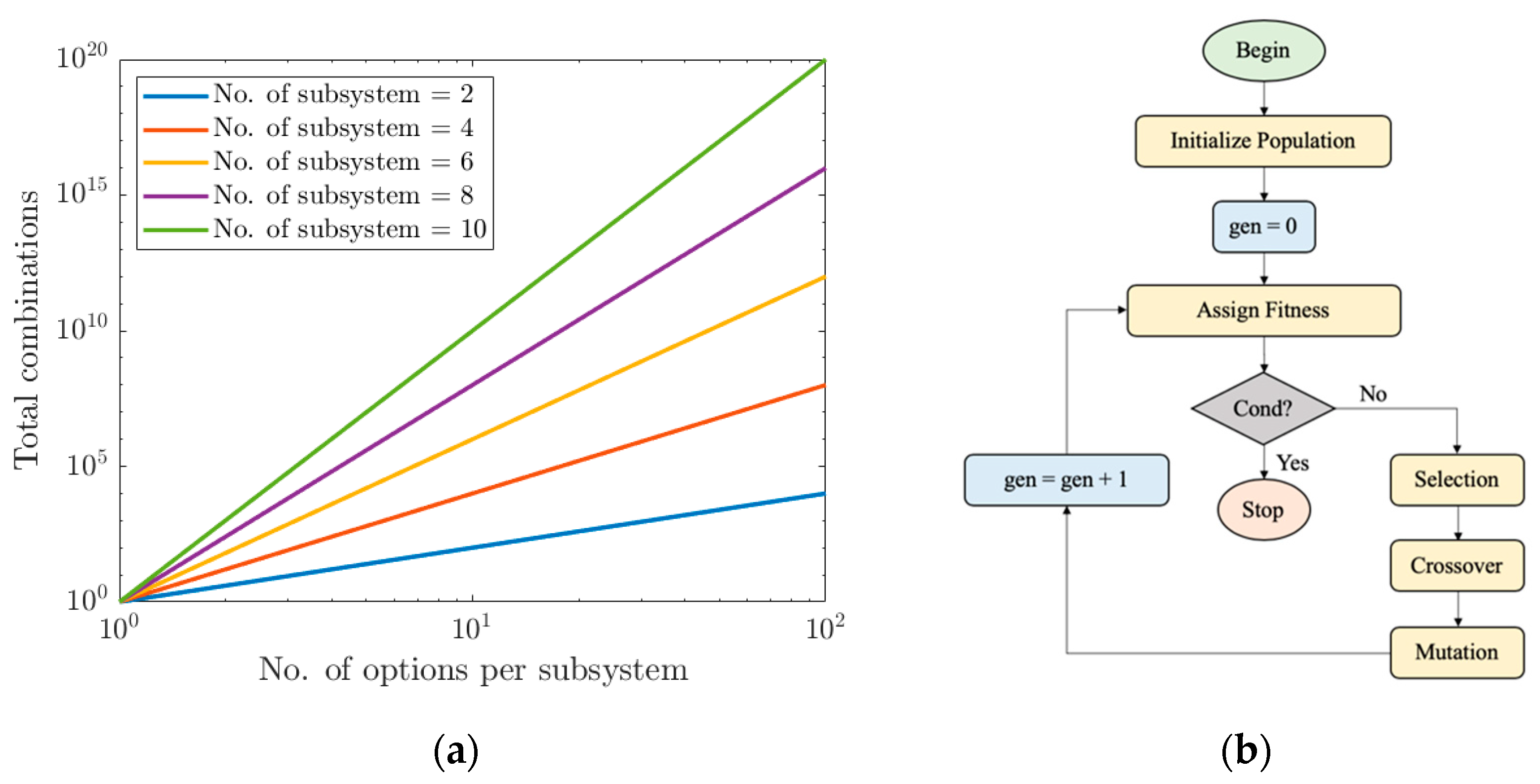
The number of possible designs, $D$, is the product of the number of options of all $n$ subsystems; $D={\displaystyle \prod }_{i=1}^n{l}_i$, which grows exponentially as the number of subsystems, $n$, and number of options, $l_i$, increases as shown in Figure 2a. One way to solve this problem is to use a brute force method by trying all $D$ possible designs, which is highly inefficient. Other methods include greedy algorithms and dynamic programming [18]. Several heuristic algorithms have also been proposed for MMKP. One such algorithm is based on the Lagrange multiplier method [20]. Other methods include HEU [21], the modified guided local search [22], the modified reactive local search [23], the convex hull-based method [24], and the column generation method [25]. Several exact algorithms have also been proposed such as the branch-and-bound method with linear programming [21] and the EMKP algorithm [26]. Although these algorithms are able to obtain fairly good solutions for small search spaces, they become ineffective due to the curse of dimensionality when approaching practical scenarios, where the number of subsystems and the number of options for each subsystem grows significantly.

However, EA provides a way to solve the knapsack problem in linear time. Evolutionary algorithms gain their inspiration from the natural process of evolution and emulate evolution by applying recombination (crossover), mutation, and natural selection on a population [27]. Highly fit individuals from the population are sampled, recombined, and resampled to form offspring of potentially higher fitness. As the evolutionary algorithm progresses through generations, fitter building blocks proliferate and unfit building blocks are culled from the population. In a way, by working with these particular schemata the complexity of the problem is reduced. Instead of building a high-performance individual by trying every conceivable combination, better and better individuals are constructed from the best partial solutions of past sampling.

Evolutionary algorithms (EAs) are a stochastic optimization method that provides an approach to learning by mimicking the metaphor of natural biological evolution or Darwinian evolution. By applying the principle of survival of the fittest, EAs progressively produce a better solution over generations by operating on a population of potential solutions. By mimicking the process of natural evolution, EAs perform evolutionary operations borrowed from natural genetics such as selection, crossover, and mutation. Theoretically, this method of evolving a population of individuals would progressively generate individuals that are better suited to their environment, just as in natural adaptation [28,29]. Figure 2b shows the structure of a simple evolutionary algorithm (EA). When successful, this approach will produce near-optimal solutions. These solutions when compared to solutions obtained through point design by a team of experts potentially presents major improvements. However, these solutions should be used as a starting point by the design team and would need further study to determine their implementation feasibility.

4. CubeSat Design

Current CubeSat design methods require a team of experts, who use their engineering expertise and decision to develop a spacecraft design from available COTS components. Such an approach may not result in an optimal design in terms of mass, volume, and power capabilities and can also miss innovative designs not thought of by the human design team. As such, the CubeSat design problem is modeled as a multidimensional multiple-choice knapsack problem. The goal is to effectively package subsystems from an inventory of COTS components within a specified mass and volume constraint such that the spacecraft can meet the defined mission goals.

As a test example, the objective is to design a 3U nadir-pointing, earth-observing CubeSat in LEO. The CubeSat is composed of many components that can be broken down into six major subsystems: (a) structure, (b) command and data handling (on-board computer), (c) communication (transceiver and antenna), (d) power (solar panels, battery pack, and power management board), (e) attitude determination and control unit (reaction wheels, magnetorquers, sun sensor, accelerometer, star tracker, magnetometer), and (f) payload (camera and lens) [1]. At first, an inventory of all the components is created from major CubeSat vendors (GomSpace, ISIS, Nanoracks, EnduroSat, DHV, NanoAvionics, Maryland Aerospace, Blue Canyon, Clydespace, Pumpkin, Space Micro, Rincon Research) which is used as a database for the Knapsack Problem. To solve the MMKP, an EA is used where a candidate population is evolved for hundreds of generations using evolutionary operators like selection, crossover, and mutation. Each individual in the population is defined by a gene, $\mathcal{G}$, which specifies what and how many components are to be packaged inside the spacecraft. This keeps the gene and design process simple and produces results fast using desktop computers. There are also other approaches to automated design, and these include the use of variable length generative coding schemes [28] that generate a constructive program to design the gene. Other bio-inspired approaches model morphogenesis [30].

An example gene structure is shown in

Table 1. Genotype of the CubeSat showing the structure of the gene: subsystem specifier; and specifier for number of batteries, and number and location of solar panels.

Structure	OBC		Antenna	Transceiver	Battery		PMB	ADCS	Solar Panel		Camera
sID	cID		aID	tID	bID		pID	adID	spID		caID
Integers $\left[\begin{array}{cc}1& l_i\end{array}\right]$: $l_i\to$ no. of options available
No. of Batteries	No. of Body Panels				No. of Deployed Panels (Side)				No. of Deployed Panels (Top)
$n_b$	b1	b2	b3	b4	ds1	ds2	ds3	ds4	dt1	dt2	dt3	dt4
Integers $\left[1 10\right]$	Integers $\left[0 1\right]$				Integers $\left[0 3\right]$

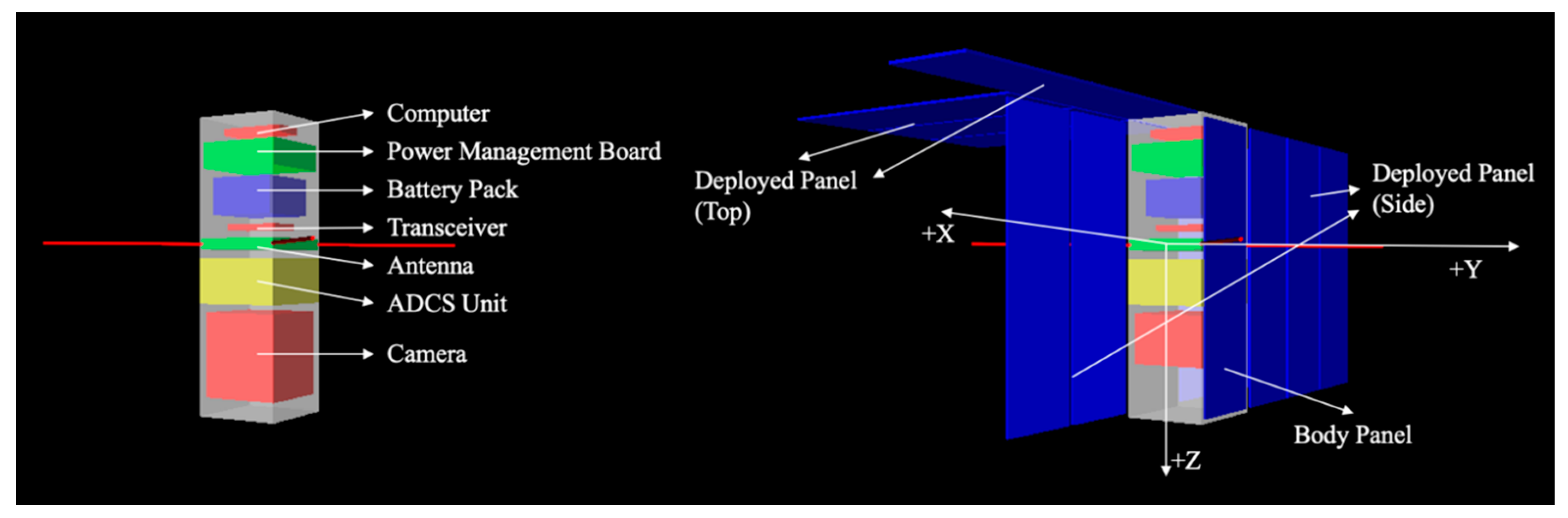
. It consists of two parts: the first part is the subsystem specifier {sID, cID, aID, tID, bID, pID, adID, spID, caID} that selects components from the available database, and the second part selects the number of batteries {$n_b$} and the number and location of solar panels: body panels {b1, b2, b3, b4}, side deployed panels {ds1, ds2, ds3, ds4}, and top deployed panels {dt1, dt2, dt3, dt4}. Figure 3 shows an example of a phenotype of the CubeSat rendered in MATLAB VRML. A script for automated assembly of all the components inside the structure is written such that each component is modeled as a cube with its maximum dimensions, and a spacing of 5 mm between components is provided for the wiring space requirement.

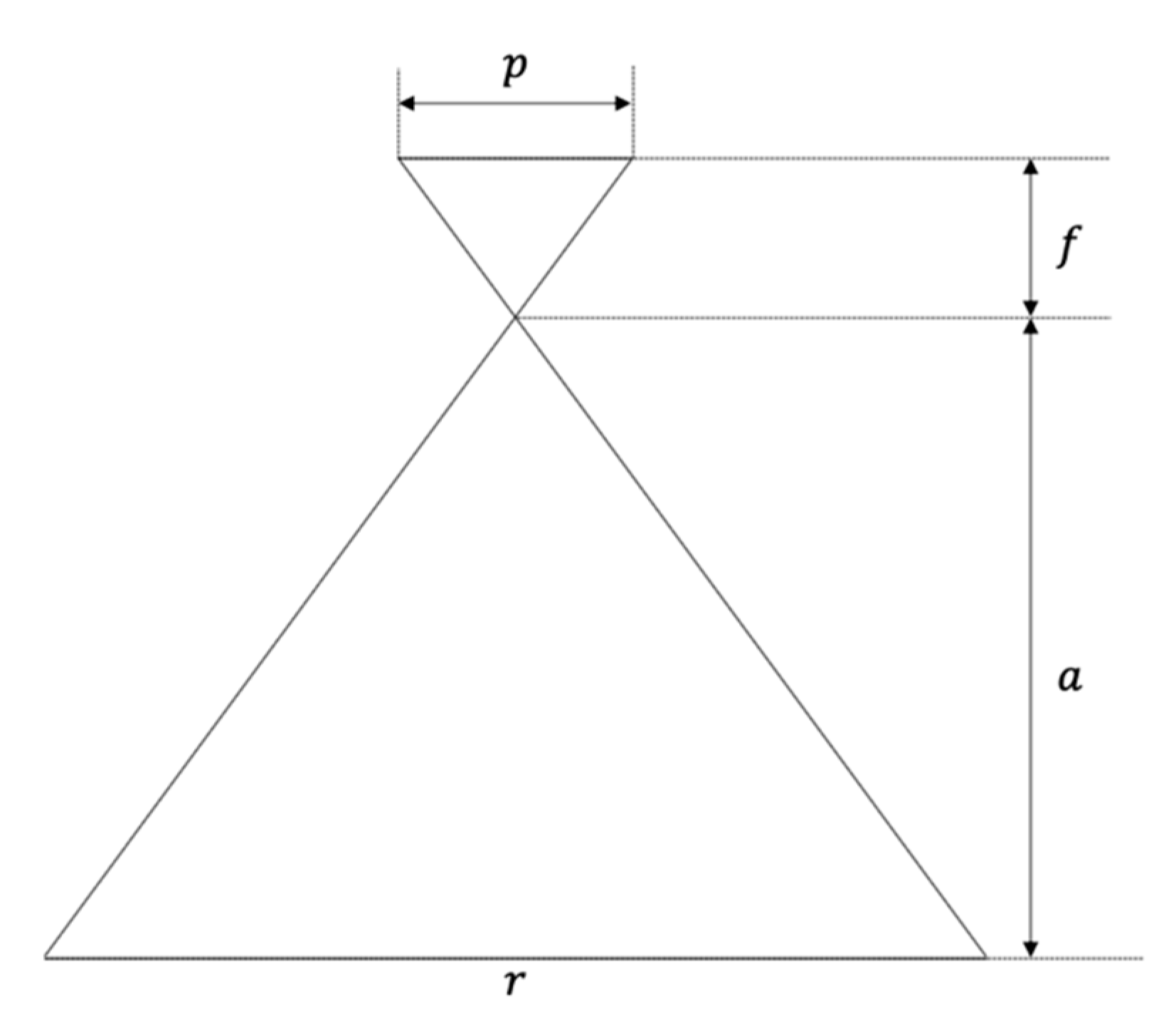
The design objective is to maximize the total downloadable ground area coverage and minimize the total mass and total cost of the satellite. For a selected camera from the inventory, the spatial resolution, $r$, is calculated as Equation (3).

$$r=\frac{ap}{f}$$

(3)

where $a$ is the altitude of the satellite, $f$ is the focal length of the lense, and $p$ is the pixel pitch of the image sensor as shown in Figure 4. Considering the sensor having $p_H\times p_V$ number of pixels, the total ground area covered per image is given by $r^2{p}_H{p}_V$ and the total size of each image is $b{p}_H{p}_V$, where $b$ is the size of each pixel. If $D$ is the total downloadable data, then the total downloadable ground area coverage, $A{C}_D$, is expressed as Equation (4).

$$A{C}_D=\frac{D}{b{p}_H{p}_V}{r}^2{p}_H{p}_V=\frac{D{r}^2}{b}$$

(4)

The mass and cost of each component is added to determine the total mass, $m_T$, and total cost, $c_T$, of the CubeSat, and thus, the objective function for the MMKP is expressed as Equation (5).

$$\min \frac{-A{C}_D}{m_T{c}_T}$$

(5)

To complete the knapsack problem, several constraints are added in terms of mass, volume, power and other properties such as the state of charge (SOC) of the battery subsystem, the pointing accuracy of the ADCS subsystem, the frequency and storage capacity of the on-board computer (OBC), and the bandwidth of the antenna and transceiver. The first constraint is such that the total mass of the CubeSat is less than the maximum allowable mass of a 3U CubeSat (4 kg). For volume constraint, three constraints are added such that after all the components are stacked inside the structure the dimensions along x, y, and z direction ($l_x,l_y,l_z$) are within the 3U CubeSat standard (10 × 10 × 34 cm) [31]. For power, two constraints are added: the first is that the average solar power generated per orbit, $P_{avg}$, should be greater than the total power requirement of the CubeSat, $P_T$, (which is determined from each component selected), and the second is that the state of charge of the battery subsystem should not drop below a minimum value (user-defined). Other constraints are also added: ADCS—pointing accuracy is within a user-defined value, OBC—clock frequency, $f_{OBC}$ and storage capacity are within some user-defined values, transceiver and antenna—bandwidth of antenna selected matches that of transceiver. The complete MMKP CubeSat design problem is then mathematically expressed as Equation (6).

$$\begin{gathered} \underset{\mathcal{G}}{\min }f\left(\mathcal{G}\right)=\frac{-A{C}_D}{m_T{c}_T} \\ \mathrm{s}.\mathrm{t}.\{\begin{array}{l}{g}_1\left(\mathcal{G}\right)\equiv m_T-4\le 0 \mathrm{kg}\\ g_2\left(\mathcal{G}\right)\equiv l_x-105\le 0 mm\\ g_3\left(\mathcal{G}\right)\equiv l_y-105\le 0 mm\\ g_4\left(\mathcal{G}\right)\equiv l_z-340\le 0 mm\\ g_5\left(\mathcal{G}\right)\equiv P_{avg}\ge P_T\equiv P_T-P_{avg}\le 0 W\\ g_6\left(\mathcal{G}\right)\equiv SOC\ge 0.2\equiv 0.2-SOC\le 0\\ g_7\left(\mathcal{G}\right)\equiv Pointing Accuracy-1°\le 0\\ g_8\left(\mathcal{G}\right)\equiv f_{OBC}\ge 730\equiv 730-f_{OBC}\le 0 \mathrm{MHz}\\ g_9\left(\mathcal{G}\right)\equiv Storage Capacity\ge 1.25\equiv 1.25-Storage Capacity\le 0 \mathrm{Gb}\\ g_{10}\left(\mathcal{G}\right)\equiv f_{trans}^{\left(L\right)}+\frac{BW}{2}\le f_{ant}\le f_{trans}^{\left(U\right)}-\frac{BW}{2}\end{array} \end{gathered}$$

(6)

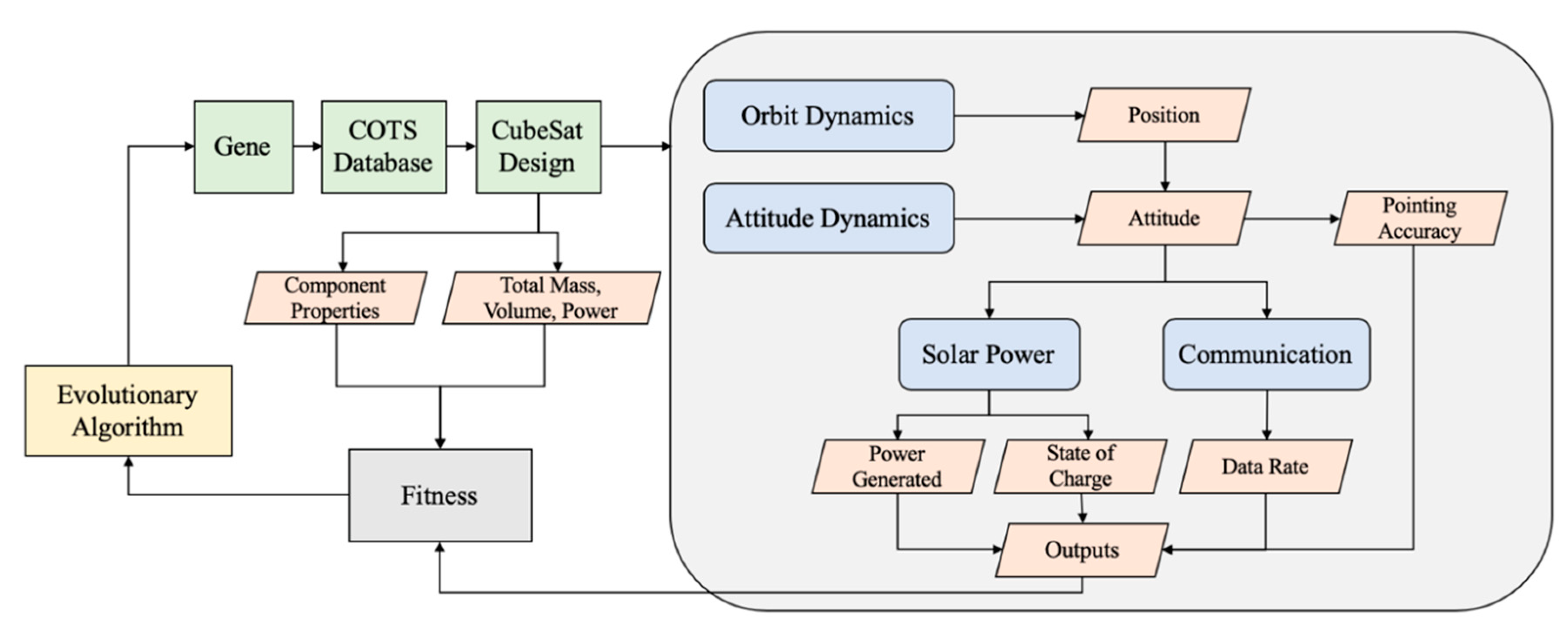
Now, to calculate the total downloadable data, $D$, average solar power generated, $P_{avg}$, state of charge of the batteries, $SOC$, and pointing accuracy of the ADCS system, a simulation environment is created that models orbit dynamics, attitude dynamics, solar power generation, battery state of charge, and communication disciplines as shown in Figure 5. Every individual of the population is an input to the COTS database that produces the CubeSat design. The design is then an input to the simulation environment, and then the outputs of the simulation environment along with mass, volume, power, and other properties of the design are used to determine the fitness (combination of objective function and the constraints). Details of the modeled disciplines are provided below.

4.1. Orbit Dynamics

The orbit-dynamics discipline computes the Earth-to-body position vector of the satellite in the Earth-centered-inertial (ECI) frame. In the orbit equation, the $J_2$, $J_3$, and $J_4$ coefficients capture the fact that the Earth is not a perfectly spherical and homogeneous mass and is expressed by Equation (7).

$$\begin{gathered} \ddot{\overrightarrow{r}}=-\frac{\mu }{r^3}\overrightarrow{r}-\frac{3\mu J_2{R}_e^2}{2r^5}\left[\left(1-\frac{5r_z^2}{r^2}\right)\overrightarrow{r}+2r_z\widehat{z}\right]-\frac{5\mu J_3{R}_e^3}{2r^7}\left[\left(3r_z-\frac{7r_z^3}{r^2}\right)\overrightarrow{r}+\left(3r_z-\frac{3r^2}{5r_z}\right)r_z\widehat{r}\right]+ \\ \frac{15\mu J_4{R}_e^4}{8r^7}\left[\left(1-\frac{14r_z^2}{r^2}+\frac{21r_z^4}{r^4}\right)\overrightarrow{r}+\left(4-\frac{28r_z^2}{3r^2}\right)r_z\widehat{z}\right] \end{gathered}$$

(7)

where $\overrightarrow{r}$ is the position vector of the satellite in the ECI frame, $\mu$ is Earth’s gravitational parameter, $R_e$ is Earth’s radius and $J_2$, $J_3$, and $J_4$ are orbit perturbation coefficients. The $J_2$, $J_3$, and $J_4$ terms must be considered because their effect is to rotate the orbit plane, which affects the power generation and communication discipline.

4.2. Attitude Dynamics

Since the CubeSat is an earth observing satellite, it must always maintain a nadir-pointing orientation. The attitude dynamics is simulated based on the reaction wheels/magnetorquers available in the selected ADCS system from the COTS inventory according to Equation (8).

$$J_s{\dot{\overrightarrow{\omega }}}_s=-{\overrightarrow{\omega }}_s\times \left(J_s{\overrightarrow{\omega }}_s+J_{RW}{\overrightarrow{\omega }}_{RW}\right)+{\tau }_{RW}+{\tau }_m+{\tau }_d$$

(8)

where $J_s$ is the moment of inertia matrix of the satellite, ${\overrightarrow{\omega }}_s$ is the angular velocity vector of the satellite, $J_{RW}$ is the moment of inertia matrix of the reaction wheel system, ${\overrightarrow{\omega }}_{RW}$ is the angular velocity vector of the reaction wheel system, ${\tau }_{RW}$ is the torque applied by the reaction wheels system, ${\tau }_m$ is the torque applied by the magnetorquers, and ${\tau }_d$ is the external disturbance torques, which is a sum of the gravity gradient, aerodynamic, and solar radiation pressure disturbances. The simulation of the attitude dynamics based on the selected ADCS system provides the pointing accuracy of the satellite, which is used for the optimization problem.

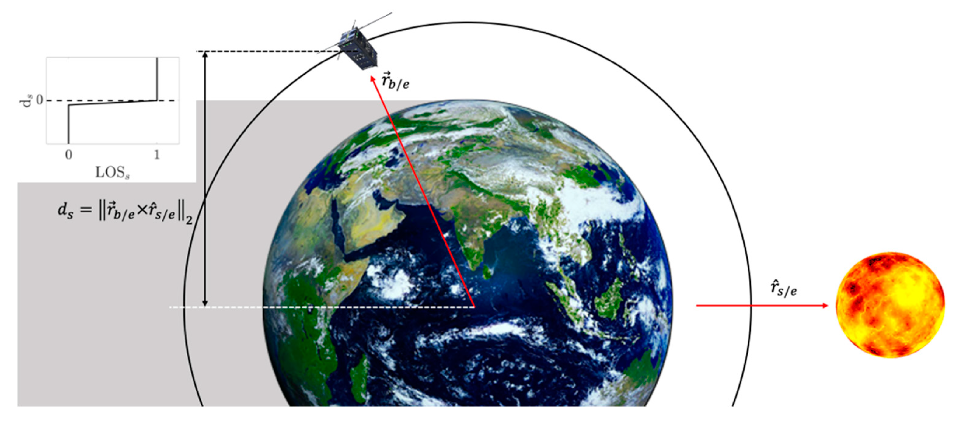
4.3. Solar Power Generation

For solar power, first the sun-to-satellite line-of-sight, $LO{S}_s$, is calculated which is essentially a multiplier for the solar panel exposed area to calculate the solar power generated. The $LO{S}_s$ is 0 if the satellite is in the eclipse and 1 otherwise, however, to implement the umbra and penumbra effects, the discontinuous function is smoothed by using a cubic function [32], as shown in Equation (9).

$$LO{S}_s=\{\begin{array}{cc}1& ,{\overrightarrow{r}}_{b/e}·{\widehat{r}}_{s/e}\ge 0\\ \left\{\begin{array}{ccc}1& ,& d_s>R_e\\ 3{\eta }^2-2{\eta }^3& ,& \alpha R_e<d_s<R_e\\ 0& ,& d_s<\alpha R_e\end{array}\right\}& ,{\overrightarrow{r}}_{b/e}·{\widehat{r}}_{s/e}<0\end{array}$$

(9)

where $d_s$ and $\eta$ are given by Equation (10).

$$d_s=\Vert {\overrightarrow{r}}_{b/e}\times {\widehat{r}}_{s/e}\Vert {}_2 \mathrm{and} \eta =\frac{d_s-\alpha R_e}{R_e-\alpha R_e}$$

(10)

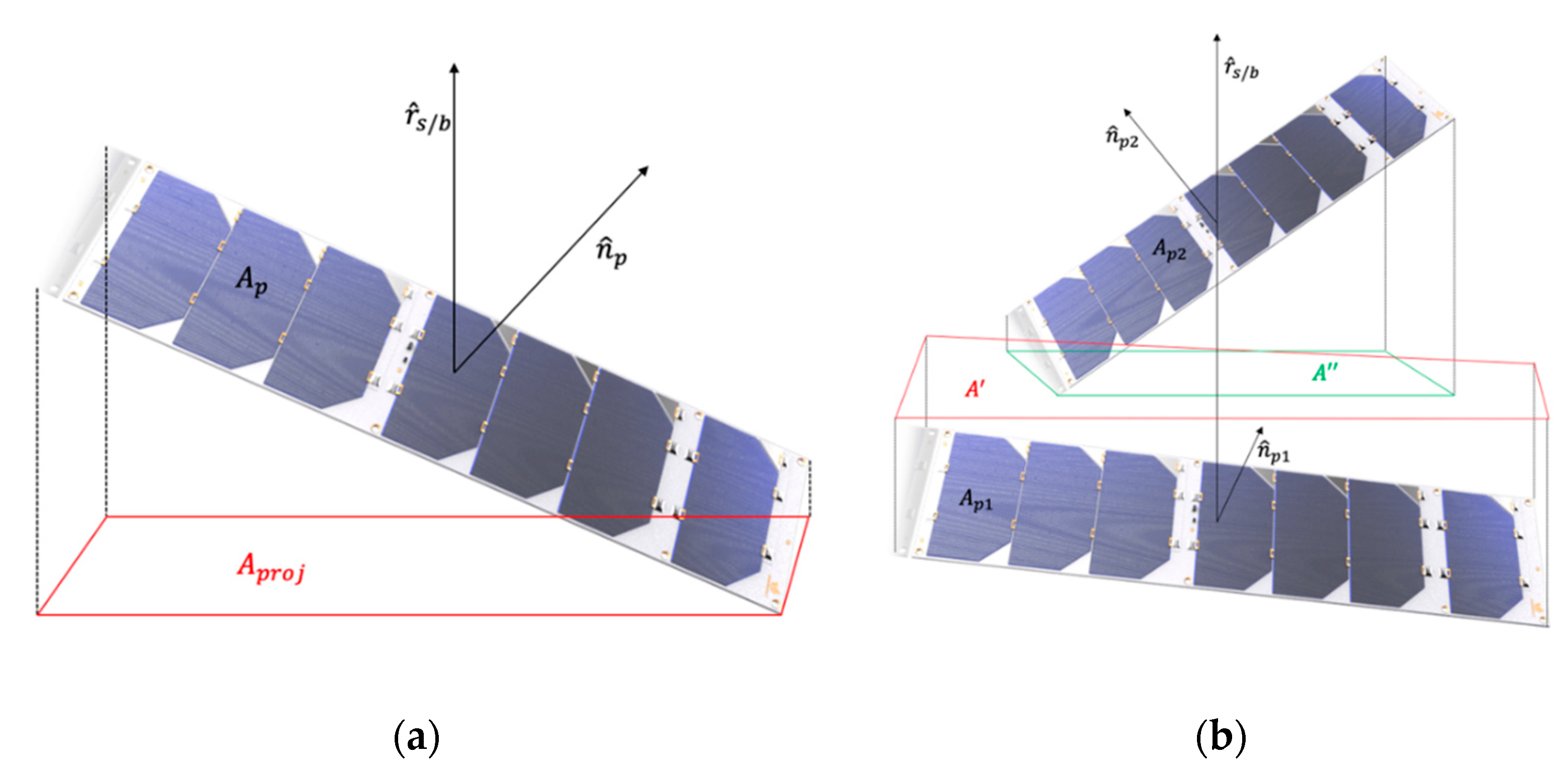
The vectors ${\overrightarrow{r}}_{b/e}$ and ${\widehat{r}}_{s/e}$ are shown in Figure 6. The value of $\alpha$ represents how far this smoothing effect extends into the Earth’s shadow, typically $\alpha =0.9$. Next, with the position of the sun known with respect to the satellite, the exposed solar panel area is required to calculate the total solar power generated. The exposed solar panel area is done in two steps. First for each panel having an area $A_p$ and unit normal vector ${\widehat{n}}_p$ and the body-to-sun unit vector ${\widehat{r}}_{s/b}$, the projected area of each panel on a plane perpendicular to ${\widehat{r}}_{s/b}$ is given by Equation (11) and shown in Figure 7a.

$$A_{proj}=\{\begin{array}{cc}{\widehat{r}}_{s/b}·{\widehat{n}}_p{A}_p& ,{\widehat{r}}_{s/b}·{\widehat{n}}_p>0\\ 0& ,{\widehat{r}}_{s/b}·{\widehat{n}}_p\le 0\end{array}$$

(11)

Next, if the satellite consists of deployable solar panels, the effects of shadows projected by one panel onto another must be considered. For two panels $\left\{\mathrm{panel} 1, \mathrm{panel} 2\right\}$ with areas $\left\{A_{p1}, A_{p2}\right\}$ and unit normal vectors $\left\{{\widehat{n}}_{p1},{\widehat{n}}_{p2}\right\}$, and body-to-sun unit vector ${\widehat{r}}_{s/b}$, the shadow cast by $\mathrm{panel} 2$ on $\mathrm{panel} 1$ is calculated by two successive projections and an intersection operator as shown in Figure 7b. The first projection is of $\mathrm{panel} 1$ on a plane perpendicular to ${\widehat{r}}_{s/b}$ given by $A^{\prime }={\widehat{r}}_{s/b}·{\widehat{n}}_{p2}{A}_{p1}$, and the second projection is of $\mathrm{panel} 2$ on a plane perpendicular to ${\widehat{r}}_{s/b}$ given by $A^{″}={\widehat{r}}_{s/b}·{\widehat{n}}_{p1}{A}_{p2}$. Finally, the projected shadow cast by $\mathrm{panel} 2$ on $\mathrm{panel} 1$ on a plane perpendicular to ${\widehat{r}}_{s/b}$ is the intersection of areas $A^{\prime }$ and $A^{″}$, as shown by Equation (12).

$$A_{shad}=A_{p1}{{\displaystyle \cap }}^{}{A}^{″}$$

(12)

Thus, the total exposed solar panel area is expressed as Equation (13).

$$A_{exp}={\displaystyle {\displaystyle \sum }_{i=1}^n}\left(A_{\left(i\right)proj}-{\displaystyle {\displaystyle \sum }_{j=1}^k}{A}_{shad\left(j\right)}\right)$$

(13)

where $n$ is the total number of solar panels, and $j=\left\{1,\dots ,k\right\}$ are the neighboring panels for panel $i$. Finally, the solar power generated is calculated as Equation (14).

$$P_{solar}=S_0{\epsilon }_{cell}{A}_{exp}$$

(14)

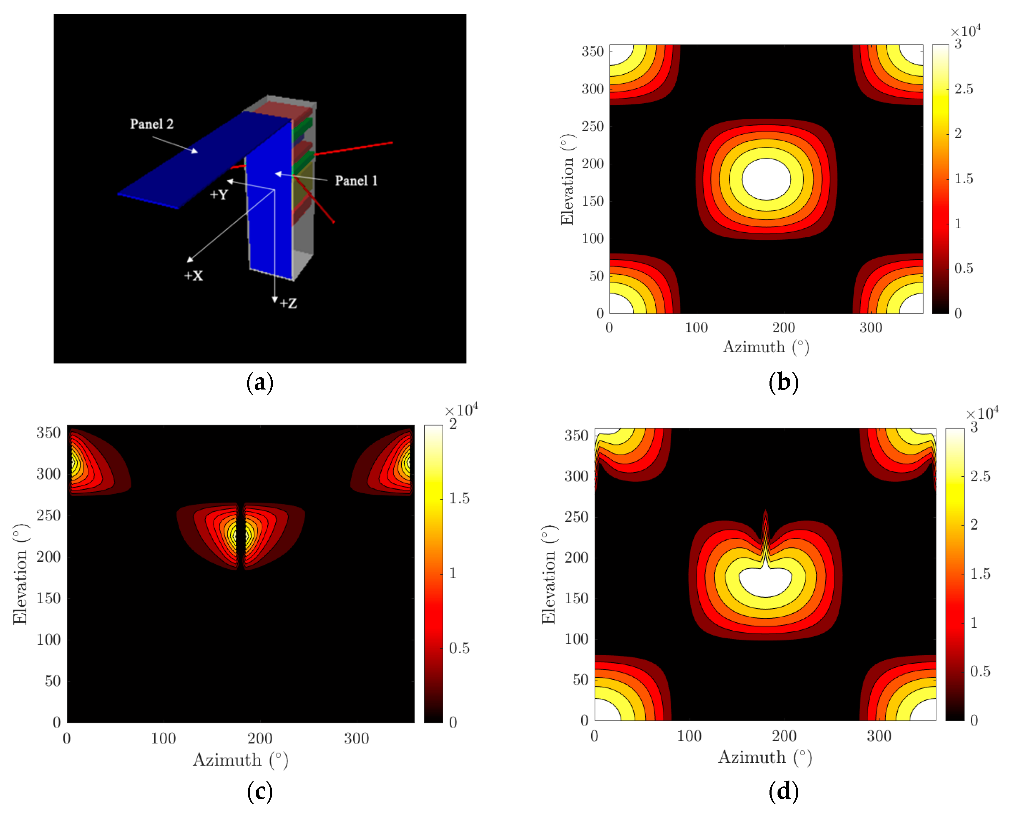
where $S_0$ is the solar constant, and ${\epsilon }_{cell}$ is the efficiency of the photovoltaic solar cells on each solar panel. Figure 8 shows the simulation results of the solar panel exposed area model for a CubeSat with two panels: one body panel and one deployed panel, as shown in Figure 8a. The simulation is performed in MATLAB, and the rendering of the CubeSat model shown in Figure 8a is done in MATLAB VRML. The body-to-sun unit vector ${\widehat{r}}_{s/b}$ is represented in a spherical coordinate system with respect to the body frame, and as such, the results are presented against azimuth and elevation angles of the sun. Figure 8b shows the exposed area of panel 1 ignoring shadows cast by panel 2, while Figure 8c shows the projected shadow cast by panel 2 on panel 1, and finally, Figure 8d shows the total exposed area of panel 1. Our method is able to calculate the total exposed solar panel area for the above CubeSat with two panels, which is used for more complicated designs evolved through the optimization process.

4.4. Battery State of Charge

The state of charge of the battery system is determined by the Ordinary Differential Equation (ODE) (Equation (15)) [32].

$$\dot{SOC}=\frac{P_{bat}}{V_{bat}Q}$$

(15)

where $Q=n_{b}q$ is the nominal discharge capacity of the battery system with $n_b$ being the number of batteries and $q$ being the discharge capacity of each battery. The dependence of the battery voltage is on the SOC and also on the temperature, which is exponential, as shown by Equation (16).

$$V_{bat}\left(SOC\right)=\left(3+\frac{e^{SOC}-1}{e-1}\right)\left(2-e^{\lambda \frac{T-T_0}{T_0}}\right)$$

(16)

where $T_0$ is the reference temperature, and $\lambda$ is the temperature decay coefficient. At any given time, the battery power is the sum of the loads, given by Equation (17).

$$P_{bat}=P_{sol}-P_{adcs}-P_{comm}-P_0$$

(17)

where $P_{sol}$ is the power generated by the solar panels, $P_{adcs}$ is the power consumed by the ADCS system, $P_{comm}$ is the communication power, and $P_0$ is the power consumed during the nominal operation of the CubeSat and the payload (camera).

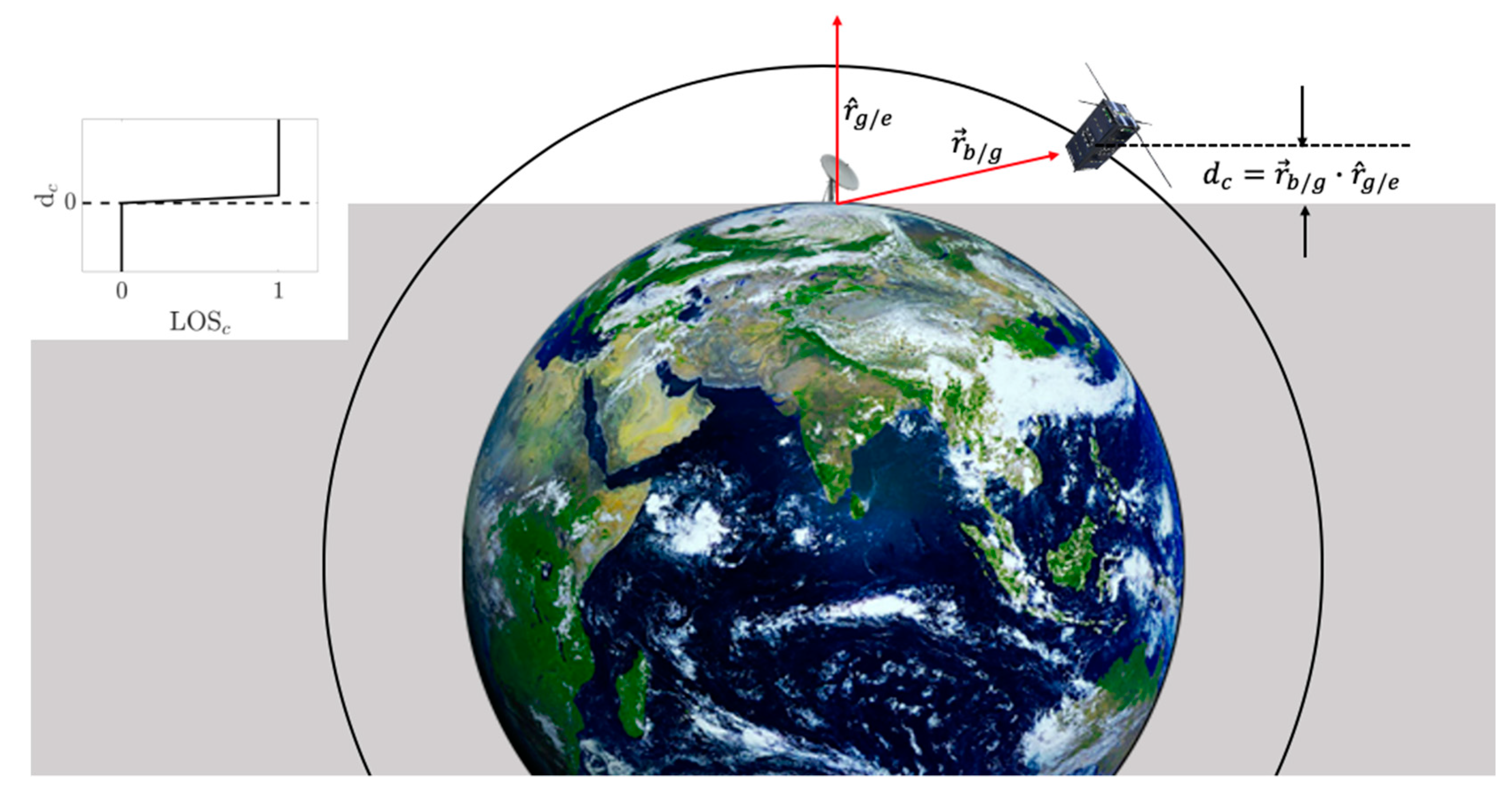
4.5. Communication

For communication, first the ground station-to-satellite line-of-sight, $LO{S}_c$, is computed based on the dot product between the Earth-to-ground station unit vector and the ground station-to-body vector in the inertial frame, as shown in Figure 9. The discontinuous function is smoothed using a cubic function. Next, the resulting data download rate, $B_r$, is calculated using Equation (18) [32,33].

$$B_r=\frac{c^2{G}_r{\eta }_p{P}_{comm}{L}_l{G}_t}{16{\pi }^2{f}^{2}k{T}_s\left(SNR\right)S^2}LO{S}_c$$

(18)

where $c$ is the speed of light, $k$ is the Boltzmann constant, $f$ is the transmission frequency, $T_s$ is the system noise temperature, $G_r$ is the receiver (ground station) gain, $SNR$ is the maximum acceptable signal to noise ratio, ${\eta }_p$ is the communication efficiency, $L_l$ is the line loss factor, $P_{comm}$ is the communication power, $G_t$ is the transmitter (satellite) gain, and $S$ is the distance from the satellite to the ground station.

4.6. Optimization

Now to solve the described CubeSat design problem implemented as a multidimensional multiple-choice knapsack problem, an evolutionary algorithm is used. The constraints described in Equation (6) divide the search space into two regions—feasible and infeasible regions. The constraints are handled using the penalty function approach. For each solution ${\mathcal{G}}^{\left(i\right)}$, $i$ being the index of the gene, the constraint violation for the inequality constraints ${\displaystyle {𝔾}_j}\left({\mathcal{G}}^{\left(i\right)}\right)\le 0$ are calculated as in Equation (19).

$$\begin{array}{c}{𝓌}_j\left({\mathcal{G}}^{\left(i\right)}\right)=\{\begin{array}{l}\left|{𝔾}_j\left({\mathcal{G}}^{\left(i\right)}\right)\right|, if {𝔾}_j\left({\mathcal{G}}^{\left(i\right)}\right)>0\hfill \\ 0 otherwise\hfill \end{array}\end{array}$$

(19)

Thereafter, all constraint violations are added together to get the overall constraint violation as in Equation (20). There are 10 constraints in the optimization problem and constraint 10 is decomposed into 2 inequality constraints.

$$\mathsf{\Omega }\left({\mathcal{G}}^{\left(i\right)}\right)={\displaystyle {\displaystyle \sum }_{j=1}^{11}}{𝓌}_j\left({\mathcal{G}}^{\left(i\right)}\right)$$

(20)

This constraint violation is then multiplied with a penalty parameter, $𝒫$, and then the product is added to each of the objective function as in Equation (21).

$$ℱ\left({\mathcal{G}}^{\left(i\right)}\right)=f\left({\mathcal{G}}^{\left(i\right)}\right)+𝒫\Omega \left({\mathcal{G}}^{\left(i\right)}\right)$$

(21)

The fitness function, $ℱ$, takes into account the constraint violations. For a feasible solution the corresponding $\mathsf{\Omega }$ term is zero and $ℱ$ becomes equal to the original objective function $f$. However, for an infeasible solution, $ℱ>f$, thereby adding a penalty corresponding to the total constraint violation. Once the fitness function is derived, the steps for an EA are used to optimize the problem. Initially, a random parent population, $P_0$, is created of size $N_P$. Each individual of the parent population comprises of the design variables represented by the gene, $\mathcal{G}$, chosen by a discrete uniform distribution ${\mathcal{G}}_j=\mathcal{U}\left({\mathcal{G}}_j^{\left(U\right)},{\mathcal{G}}_j^{\left(L\right)}\right)$, where ${\mathcal{G}}_j$ is the j-th design variable and ${\mathcal{G}}_j^{\left(U\right)}$ and ${\mathcal{G}}_j^{\left(L\right)}$ are the upper and lower bounds of the design variables. For each individual, the value of the fitness function $ℱ\left(\mathcal{G}\right)$ is evaluated using the simulation environment as shown in Figure 6. Next, the usual tournament selection, crossover, and mutation operators are used to create an offspring population, $Q_0$, of size $N_Q$ [34]. For crossover, a blend crossover (BLX-α) operator is used [35]. During mutation, we use a non-uniform mutation operator. The mutation operator is constructed such that the probability of creating a solution closer to the parent is more than the probability of creating one away from it [36]. By comparing the current population with previously found best solutions, elitism is introduced into the algorithm. For the $t^{th}$ generation, first a combined population $R_t=P_t+Q_t$ is formed. The population $R_t$ is of size $N_{ }+N_Q$. Since all previous and current population members are included in $R_t$, elitism is automatically ensured. Next, the fitness of each individual in $R_t$ is calculated according to the fitness function $ℱ\left(\mathcal{G}\right)$. Based on the value of the fitness function, the population is sorted in ascending order and the best $N$ individuals are selected for the next generation. The new population, $P_{t+1}$, of size $N$ is again used for selection, crossover, and mutation to create a new population, $Q_{t+1}$, of size $N_Q$. The process is repeated until the desired results are obtained, or the max number of generations are achieved.

5. Results

For the test case the orbit of the satellite is simulated for an altitude of 400 km, inclination of 90°, eccentricity of 0 (circular orbit), RAAN of 90°, argument of perigee of 0°, and mean anomaly of 0°. The values of the constants used in the simulation are shown in

Table 2. Constants used in simulation.

Constant	Symbol	Value
Earth’s gravitational parameter	$\mu$	398,600.44 km3·s−2
Earth’s radius	$R_e$	6378.137 km
Orbit perturbation coefficients	$J_2$	1.08264 × 10−3
	$J_3$	−2.51 × 10−6
	$J_4$	−1.60 × 10−6
Solar constant	$S_0$	1367 W/m2
Reference temperature	$T_0$	293 K
Temperature decay coefficient	$\lambda$	ln(1/(1.1)5)
Speed of light	$c$	2.99792458 × 108 m/s
Boltzmann constant	$k$	1.380648 × 10−23 m2kg/(s2K)
System noise temperature	$T_s$	500 K
Receiver gain	$G_r$	12 dB
Signal-to-noise ratio	$SNR$	5.0 dB
Communication efficiency	${\eta }_p$	0.2
Line loss factor	$L_l$	−2.0 dB
Penalty parameter	$𝒫$	100
PSO tuning parameters	$\omega$	1.1
	$\beta$	1.49
	$\gamma$	1.49
Annealing parameter	$\kappa$	5

. The optimization problem is simulated for 10 orbits in MATLAB, and the results are presented in Figure 10 and Figure 11.

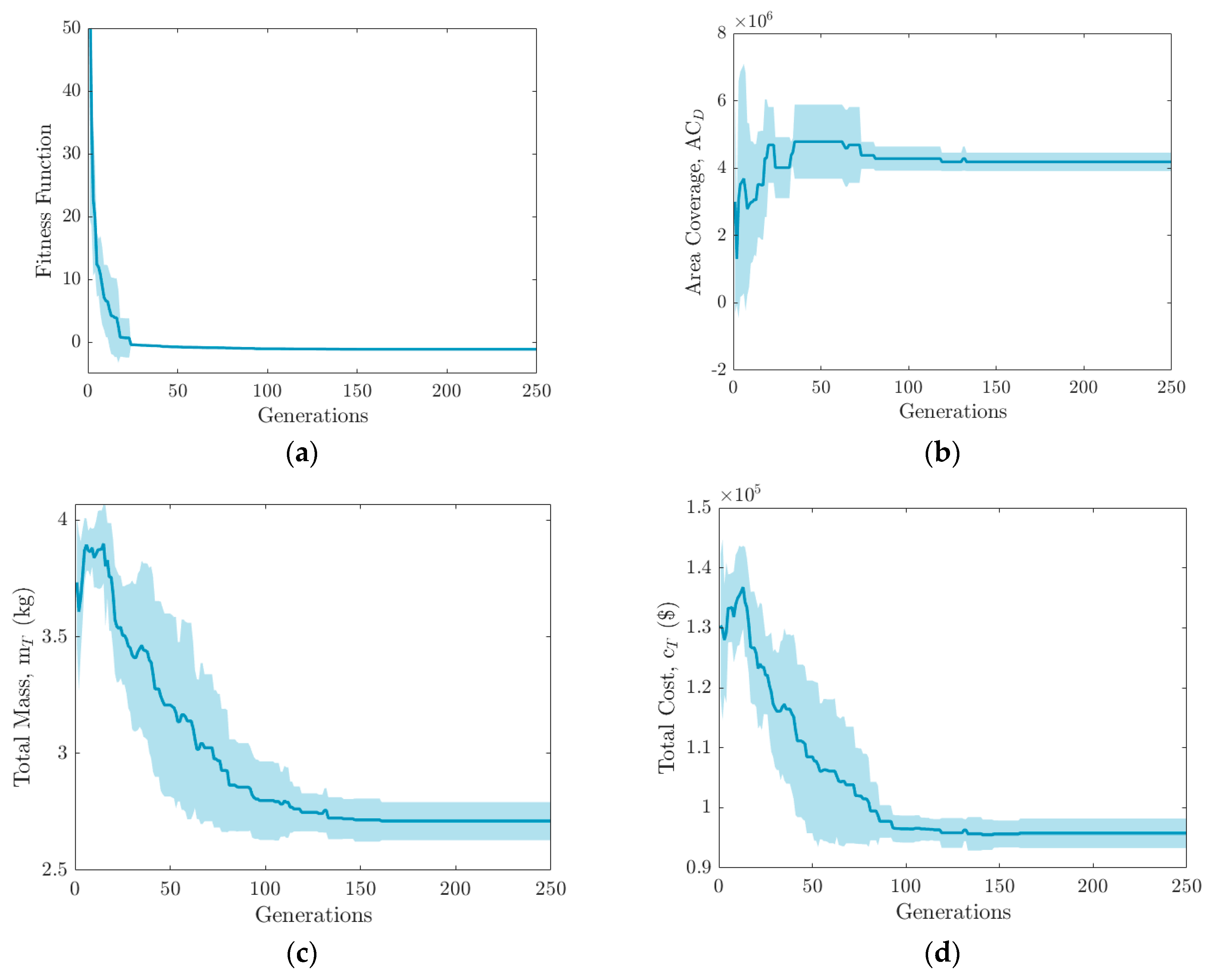
Figure 10a shows the evolution of the fitness function $ℱ\left(\mathcal{G}\right)$ over 250 generations with 100 populations in each generation. Figure 10b shows the evolution of the total downloadable ground area coverage, $A{C}_D$, Figure 10c shows that of the total mass, $m_T$, and Figure 10d shows that of the total cost, $c_T$, of the CubeSat over 250 generations. The shaded region of each of the plots show the 95% confidence interval over 20 runs. The results of the plots show that the fitness function decreased with generations converging to a constant fitness, while the total downloadable ground area coverage increased, and the total mass and total cost decreased with generations as implemented in the optimization problem.

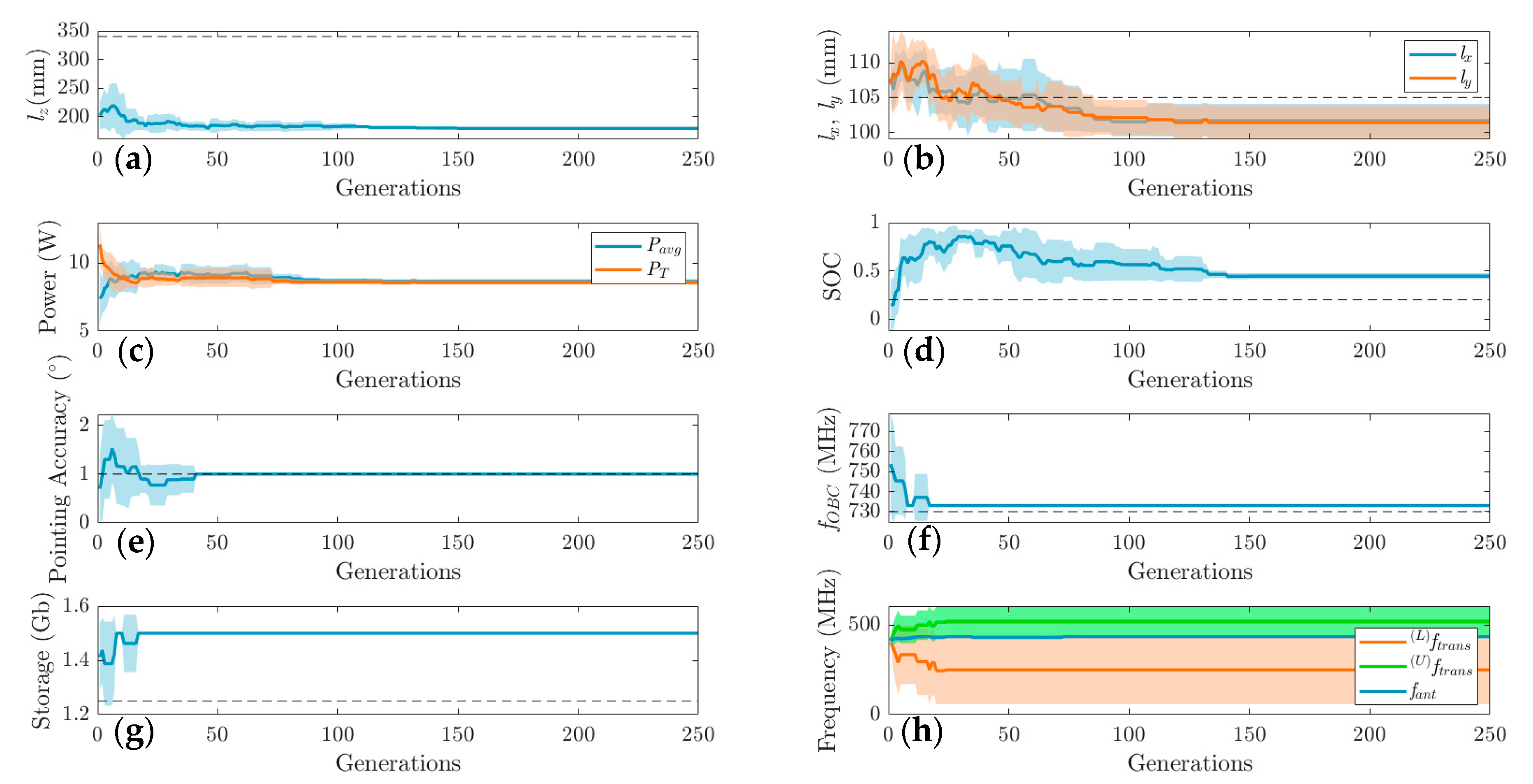
Figure 11 shows the evolution of the constraints $g_2$ to $g_{10}$. The constraint $g_1$ is already presented in Figure 10c, which shows that the total mass is below the 4 kg allotted mass of a 3U CubeSat. Figure 11a,b shows the evolution of the dimension of the assembled CubeSat components along z, x, and y directions, showing it is within the 340 mm and 105 mm limit (shown by the dashed lines). Figure 11c shows the evolution of the average solar power generated per orbit, $P_{avg}$, and the total power requirement of the CubeSat, $P_T$, satisfying the requirement $P_{avg}\ge P_T$. Figure 11d shows the evolution of the state of charge, SOC, of the battery system with the dashed line showing the minimum requirement of 0.2. Figure 11e shows the evolution of the pointing accuracy of the ADCS system, which satisfies the constraint $Pointing Accuracy\le 1°$. Figure 11f,g shows the evolution of the clock frequency and storage capacity of the on-board computer, which are greater than the specified values of 730 MHz and 1.25 Gb, respectively (shown by the dashed lines). Figure 11h shows the evolution of the antenna frequency ($f_{ant}$) along with the upper ($f_{trans}^{\left(U\right)}$) and lower ($f_{trans}^{\left(L\right)}$) limit of the frequency of the transceiver, showing the antenna frequency is within the limit of the bandwidth of the transceiver. It is clearly evident that all the constraints have been satisfied when the optimization process was terminated, and as such, the final solutions found are in the feasible region of the design space.

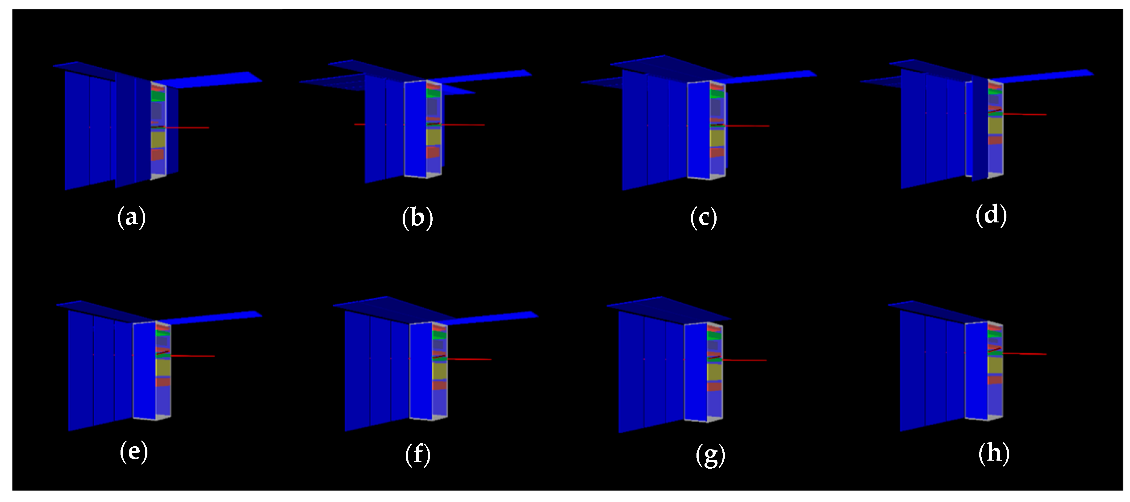
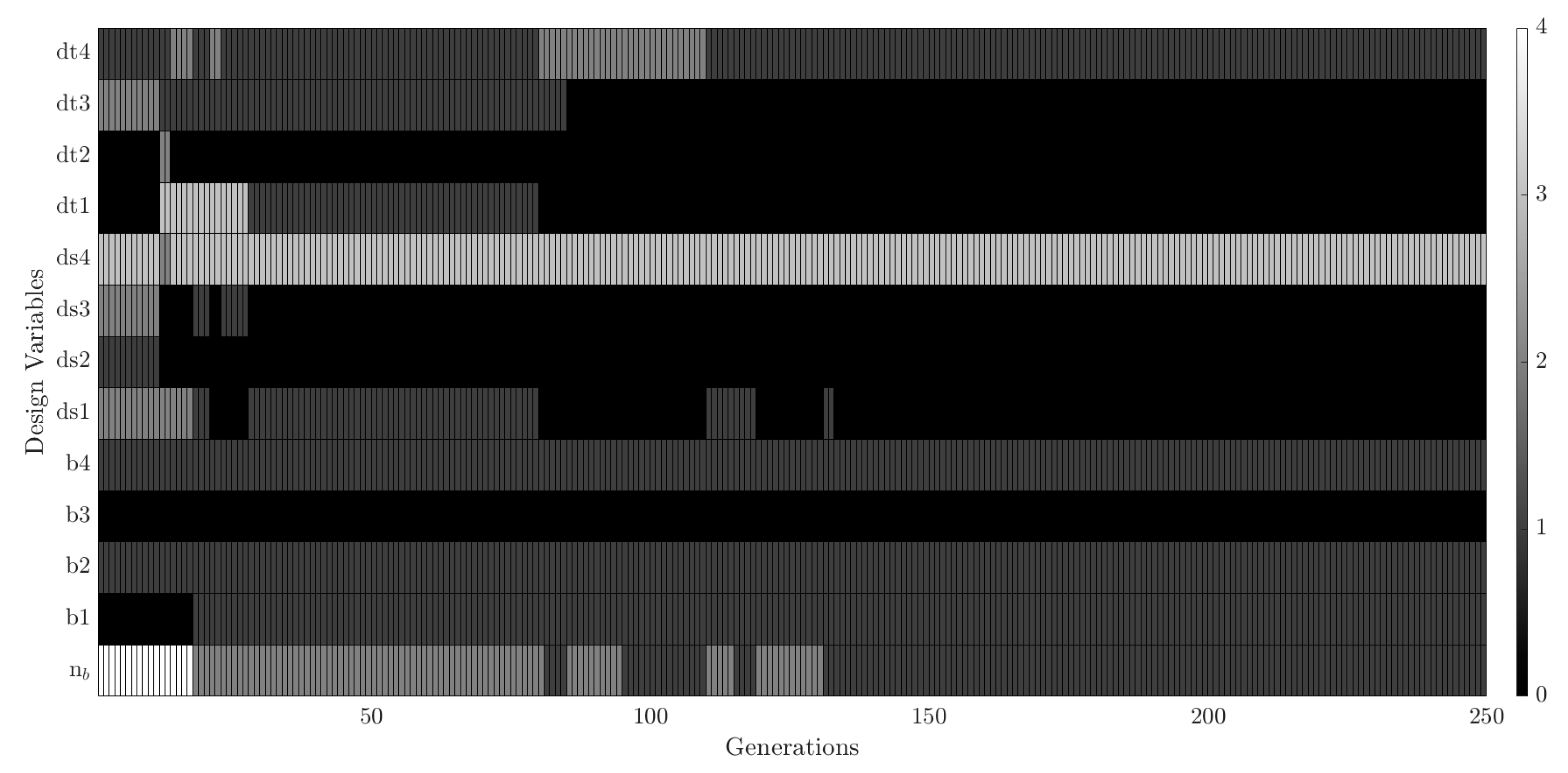
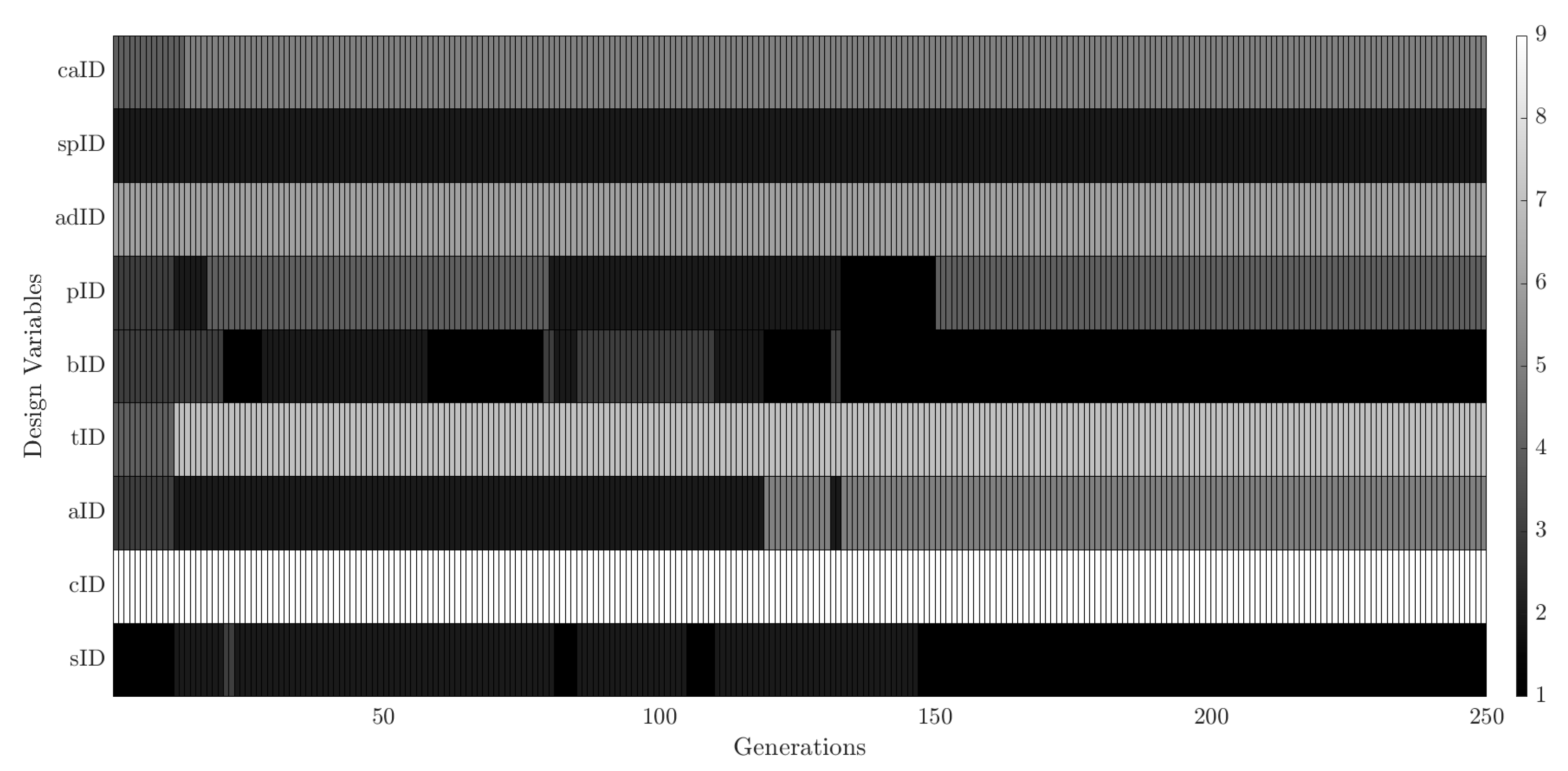
Figure 12 shows the rendering of the evolution of the best design over generations 1, 12, 15, 20, 30, 80, 100, and 150. It can be seen that the number of solar panels and their positions changed over generations, and at the same time, the internal components vertically stacked inside the structure also changed. Figure 13 and Figure 14 show the variation of the design variables (represented by the gene in Figure 3) of the best individual over generations. The color of the design variables represents the component selected from the inventory in Figure 13 and the number of batteries and solar panels in Figure 14. It can be seen that the combination of the subsystems and the number of batteries and solar panels changed until generation 150, and then an optimal combination was found.

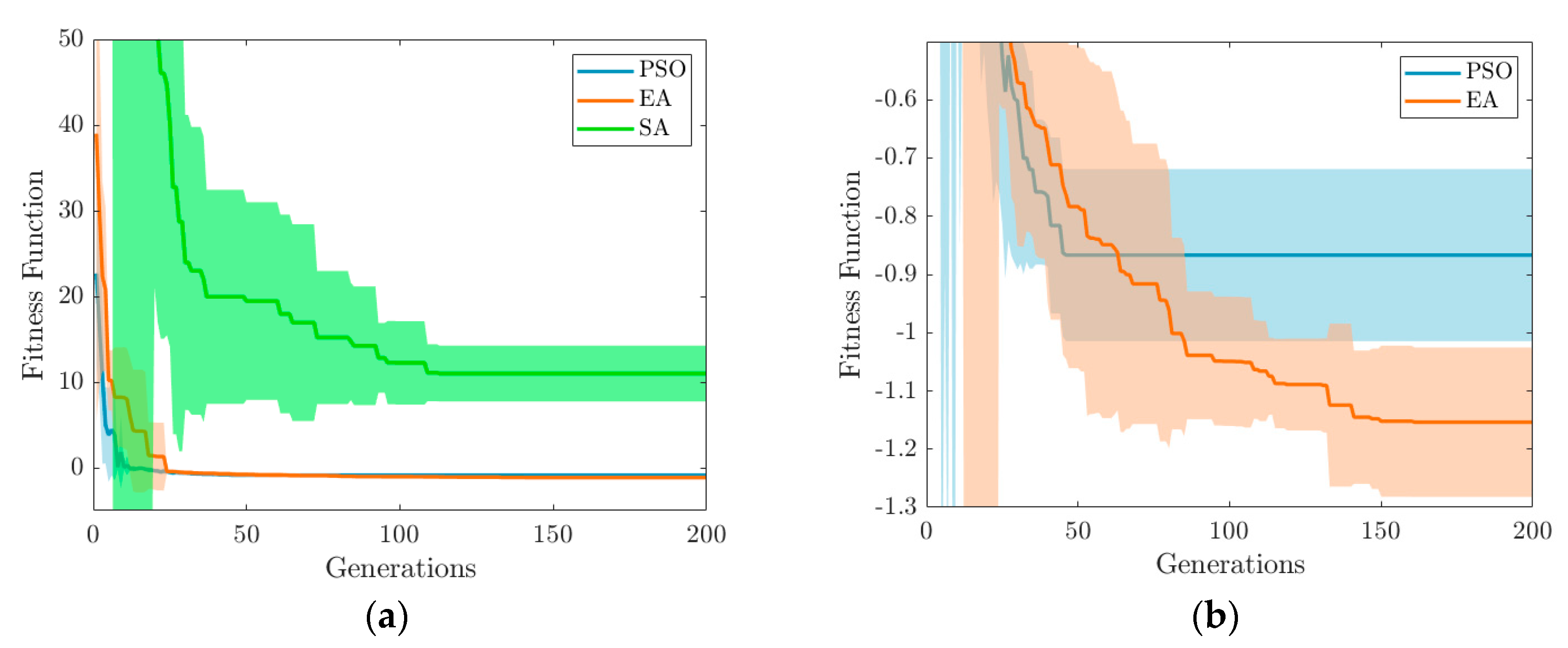
Finally, we present a comparative analysis between three stochastic algorithms, evolutionary algorithm (EA), particle swarm optimization (PSO) [37], and simulated annealing (SA) [38], in terms of performance on the CubeSat design MMKP problem. The theory behind the application of the EA to our design problem has already been discussed in the preceding sections. We now provide a brief explanation on how PSO and SA are implemented.

5.1. Particle Swarm Optimization

Particle swarm optimization is a stochastic optimization method that is inspired from the social behavior of fish schooling or birds flocking. Just like EA, PSO is also initialized with a population (swarm) of individuals (particles). However, unlike EA, PSO does not use evolutionary operations to search for optima; instead, each particle is guided through the search space in every iteration by updating their positions and velocities using better positions found by other particles. In our CubeSat design problem, the fitness is defined by Equation (21) as $ℱ\left({\mathcal{G}}^{\left(i\right)}\right)$, where ${\mathcal{G}}^{\left(i\right)}$ is the position of each particle, and the velocity of each particle is denoted by ${\mathcal{V}}^{\left(i\right)}$. The algorithm is initialized by generating $N$ particles with their positions and velocities initialized randomly. Next, at every iteration, $t$, the velocity and position of each particle are updated by Equations (22) and (23), respectively.

$${\mathcal{V}}_{t+1}^{\left(i\right)}=\omega {\mathcal{V}}_{t+1}^{\left(i\right)}+\beta r_1\left(p_t^{\left(i\right)}-{\mathcal{G}}_t^{\left(i\right)}\right)+\gamma r_2\left(p_t^{\left(g\right)}-{\mathcal{G}}_t^{\left(i\right)}\right)$$

(22)

$${\mathcal{G}}_{t+1}^{\left(i\right)}={\mathcal{G}}_t^{\left(i\right)}+{\mathcal{V}}_{t+1}^{\left(i\right)}$$

(23)

where $\omega$, $\beta$, and $\gamma$ are the tuning parameters, $r_1$ and $r_2$ are random numbers generated between 0 and 1, $p_t^{\left(i\right)}$ is the best remembered individual particle position, and $p_t^{\left(g\right)}$ is the best remembered swarm position. This process of updating the position and velocity of each particle continues until the desired fitness is achieved or maximum number of iterations reached.

5.2. Simulated Annealing

Simulated annealing is another stochastic optimization method that is inspired from annealing in metallurgy. The algorithm starts with a random trial solution, $\mathcal{G}$, whose fitness is determined by $ℱ\left(\mathcal{G}\right)$, defined by Equation (21), and a large initial temperature, $T_0$. At each iteration, $t$, the algorithm randomly generates a new solution, ${\mathcal{G}}_{t+1}$, and its corresponding fitness, $ℱ\left({\mathcal{G}}_{t+1}\right)$, is calculated. If the new solution is better than the current solution, it is automatically selected as the next solution. However, if the new solution is worse, the algorithm accepts it as the next solution based on a probability of acceptance function defined by Equation (24).

$$P\left({\mathcal{G}}_{t+1}\right)=\frac{1}{1+\exp \left(\frac{∆}{\max \left(T\right)}\right)}$$

(24)

where $∆=ℱ\left({\mathcal{G}}_{t+1}\right)-ℱ\left({\mathcal{G}}_t\right)$ and $T$ is the current temperature, which is systematically lowered by the algorithm at each iteration according to Equation (25).

$$T=\frac{T_0}{\ln \left(\kappa \right)}$$

(25)

where $\kappa$ is the annealing parameter. Since the values of Δ and $T$ are positive, larger Δ and a lower temperature leads to a smaller acceptance probability. The algorithm stores the best solution found so far and proceeds until the desired fitness is achieved or maximum number of iterations reached.

Figure 15a shows the evolution of the mean and standard deviation of fitness function over generations for all the 3 algorithms simulated and averaged over 20 times. The constant parameters used for PSO and SA are presented in Table 2. It can be clearly seen that the optimal solution found using simulated annealing lies in the infeasible region as the fitness function is positive. Both the evolutionary algorithm and particle swarm optimization were able to find a feasible solution, but the performance of the EA is better than PSO, as shown in Figure 15b, making it the better choice for this problem. Our observations show PSO stagnates prematurely, while EAs are more effective in continuing to innovate over generations.

6. Conclusions

This paper provides an analysis of the use of evolutionary algorithms to design complex systems that consist of multiple subsystems. It utilizes an inventory of components that are made available for each subsystem. The mathematical formulation for designing such a system is presented as a multidimensional multiple-choice knapsack problem (MMKP). The number of possible designs for a MMKP problem increases exponentially as the number of subsystems and number of options available for each subsystem increases. As such, the use of stochastic methods such as evolutionary algorithms (EAs) that mimic the metaphor of natural biological evolution provides a way to solve the problem in linear time complexity. A CubeSat design problem is presented as an example and an evolutionary algorithm is successfully applied in finding near-optimal designs. The approach has the potential for producing designs that maximize a mission-specific cost function while minimizing cost and mass. Traditionally, mission concepts are created by a team of engineers by conducting trade studies for mass, cost, volume, performance, and risk. Our approach of automated design using evolutionary algorithms for trade space selection speeds up the design process. Moreover, it provides us with a better basis for detailed system architecture, and hence, better design decisions can be made with confidence. This method generates a set of near-optimal designs, which provides multiple designs to start with and potentially presents vast improvements over a solution obtained through engineering judgement and point design alone. Our EA approach also shows improvement over other stochastic optimization methods including particle swarm optimization (PSO) and simulated annealing (SA). Although our approach shows a credible pathway to identify and evaluate many more candidate designs, these optimized designs will need further study to determine their implementation feasibility.