1. Introduction
Today’s aircraft manufacturers are eager to fulfill the greener imperative demanded by society and allow for a more economic operation of aircraft. Besides the efficiency of engines and aerodynamics, the aircraft weight and the wing aspect ratio have a major impact on the fuel consumption. A reduction of aircraft weight is achieved by using new materials like carbon composites, as it has been successfully achieved for example with the Airbus A350 or the Boeing 787, where higher aspect ratios yield reduced aerodynamic drags. These approaches, however, decrease the aircraft velocity at which undesired effects like flutter, i.e., the unstable coupling between the aerodynamics and the aircraft structure, occur. If the trend of reducing the aircraft structure is continued, these effects will appear within the desired flight envelopes. Possible countermeasures are active control techniques which allow for stabilizing these unstable dynamics and extending the operational region of the aircraft. Such advanced control algorithms require model-based design methods which call for adequate models of the aeroservoelastic effects. Thus, the design of flutter suppression controllers is a challenging task and has raised attention to the academic community, see for example [
1,
2,
3] for valuable contributions. In this article, the design of a flight control system including the baseline and flutter suppression controller for a highly flexible flutter demonstrator is presented. The considered aircraft, depicted in
Figure 1, is the main demonstrator of the Horizon 2020 project Flutter Free FLight Envelope eXpansion for ecOnomic Performance improvement (FLEXOP) to develop and test active flutter suppression control algorithms [
4,
5].
The proposed control system features two main parts, the baseline flight control system to navigate the aircraft fully autonomously around the predefined flight test track and the active flutter control algorithms to stabilize the aircraft’s flutter modes thereby extending its operational range. The architecture of the presented baseline controller to augment the rigid body motion features a classical cascaded flight controller architecture [
6,
7,
8] with well proven feedback loops of proportional-integral-derivative (PID) controllers together with damping augmentation. These control loops provide capabilities for augmented pilot-in-the-loop flights as well as for autonomous flights. A major task during the design of active flutter suppression algorithms is the adequate fusion of the numerous available measurements on the wings and the different control inputs. This is commonly done in a pre-processing step by the control engineer before deriving the control algorithm. In
Section 2 of this article, a new systematic approach to analytically blend the available inputs and outputs to isolate the aeroelastic modes to be stabilized is presented. This enables a simple control design for each individual mode, using parametrized single-input single-output (SISO) controllers of a predefined structure.
By defining the structure of the controllers in advance, the design of the flutter suppression controller as well as the baseline controller reduces the selection of adequate control gains. For this selection a model-based approach using robust control techniques is proposed in
Section 3. Two generic control design problems are defined: the first problem defines a multi-model, multi-objective optimization for deriving a controller which is robust against parameter variations. The second design is posed as parametric multi-objective problem for designing gain-scheduled controllers. Both problems are solved using non-smooth optimization based on robust control algorithms [
9]. In the case of the gain-scheduled controller, this approach enables the direct determination of the controller parameters over the entire flight envelope in a single design step, i.e., avoiding the classically applied point-wise design. The presented tool chain for the controller design is applied to the FLEXOP flutter demonstrator in
Section 4. A detailed overview of the baseline controller functionality and the employed loops and design criteria is provided. Furthermore, the application of the proposed blending vector design and parameter tuning to derive the flutter suppression controller is discussed, providing valuable insight to the reader on how such algorithms are developed. The designed flight control system of the FLEXOP flutter demonstrator is verified in an extensive verification campaign and its results are reported in
Section 5. For the verification campaign a high fidelity, non-linear simulator of the closed-loop aircraft [
10,
11], including structural and aerodynamic effects as well as detailed actuator, sensor and engine models, is available. The verification includes wind scenarios to test the disturbance attenuation, acceleration scenarios to verify the stabilization capabilities of the active flutter control algorithm, and flights along the predefined flight test pattern on which the real flight tests will be performed.
2. -Optimal Input and Output Blending
In this section, the theoretical background to optimally blend inputs and outputs of a system is provided. The approach blends the inputs and outputs in a way that the controllability and observability of the mode to be controlled is maximized in terms of the -norm. For aeroelastic control problems, this approach is especially applicable since no model order reduction of the typically high dimensional aeroelastic model is required. Furthermore, a high number of sensors, e.g., strain or acceleration measurements, are available and need to be fused accordingly within the control algorithm.
2.1. Modal Control of Linear Time-Invariant Systems
A linear time-invariant (LTI) system with
inputs,
outputs and
states which is physically realizable is described by the transfer function matrix
where
and
s denotes the Laplace variable. Assuming that
is diagonalizable, a modal decomposition of
is possible such that
where the individual modes
are given as
According to Equation (
2), a mode
m is either described by a single real pole
with an imaginary part
or a conjugate complex pole pair
and
. Hence, the number of modes
does not necessarily equal the number of states
, i.e.,
. Each pole
is associated with a residue
, where the residues of a conjugate complex pole pair are also conjugate complex.
In general, a mode
m is considered to be asymptotically stable if
and unstable if
. In case
, the mode is considered to be undamped, which also includes a pole in the origin. Furthermore, the natural frequency of a mode is given as
and for
, the corresponding relative damping is
. Please note that for a conjugate complex pole pair, the corresponding real parts
and magnitudes
are equal. For more information on modal decomposition and the properties of individual modes see, for instance, [
12].
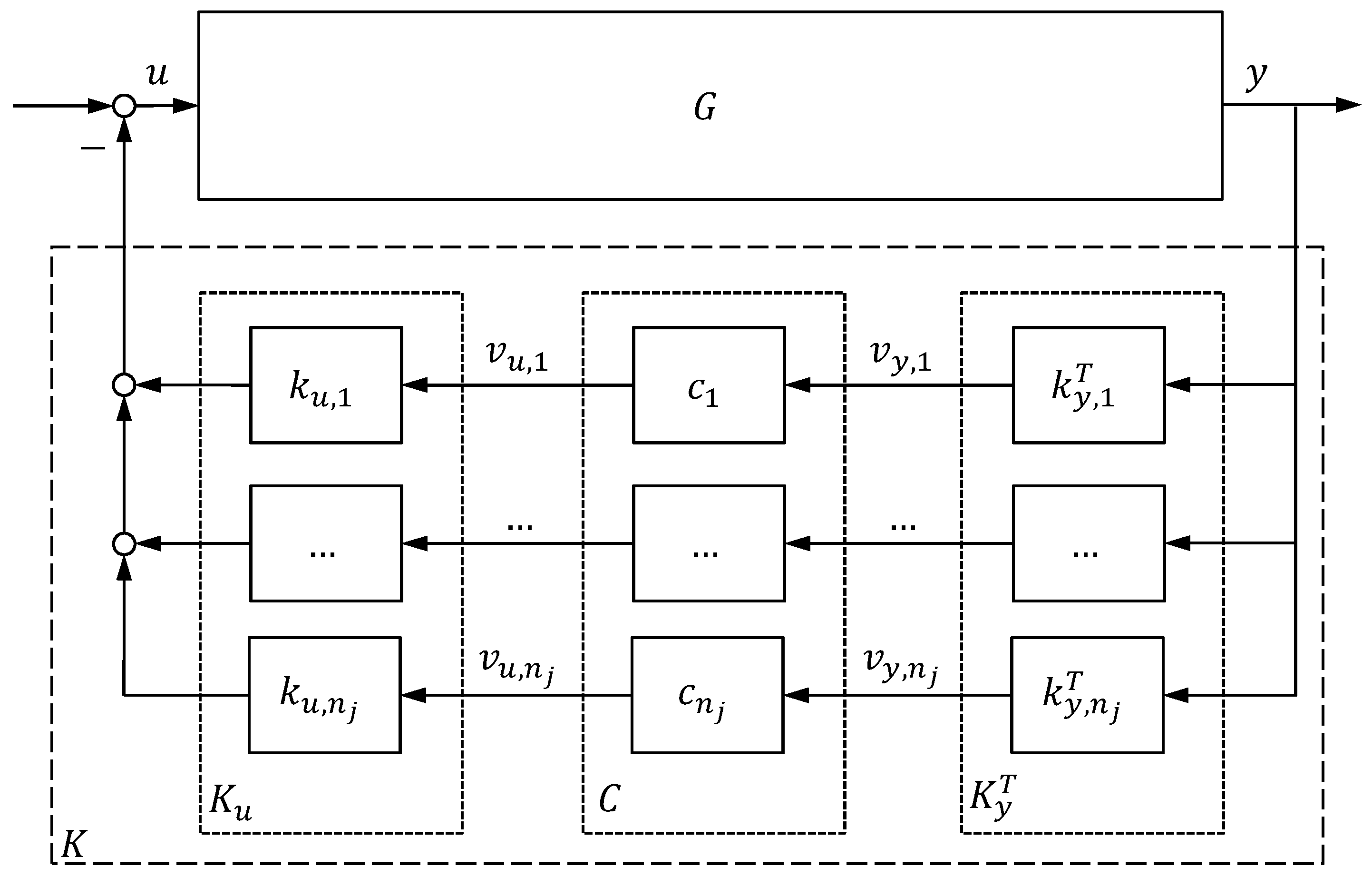
The task of controlling a single mode of a high order dynamic system is challenging when the number of control inputs or measurement outputs is increased. To reduce the complexity of the control problem, it is proposed to weight and sum the measurement signals such that the resulting virtual measurement output represents the response of the mode to be controlled. Similarly, it is proposed to generate a virtual control input which is distributed to available control inputs such that the target mode are individually controlled. In other words, the mode to be controlled is isolated by blending inputs and outputs. The corresponding input and output blending vectors and depend on the shape of the targeted mode and are seen as directional filters. This implies a high robustness against frequency variations as the blending vectors are independent of the mode’s natural frequency. Blending the inputs and outputs as proposed, a simple single input and single output (SISO) controller is designed to control the isolated mode. Hence, the multiple inputs and multiple outputs (MIMO) control design problem becomes a SISO one with the challenge to find adequate blending vectors.
In
Figure 2, the resulting feedback interconnection is depicted, where the modes
are subject to be controlled. Summarizing the input and output blending vectors in
and
, the overall controller is
where the SISO controllers are collected on the diagonal of
.
2.2. -Optimal Blending Vector Design
The goal addressed herein is to find blending vectors which yield a maximum controllability and observability of the mode to be controlled in terms of the -norm. This requires a joint design of the input and output blending vectors as controllability and observability cannot be regarded independent of each other. Furthermore, the proposed method is extended to undamped and unstable modes, for which the -norm becomes infinite by definition.
In this article, the combined controllability and observability of an asymptotically stable mode
is quantified in terms of the
-norm. Hence, the goal is to stay as close as possible to the original controllability and observability of the targeted mode when blending inputs and outputs with real-valued unit vectors
and
, respectively. This gives rise to quantify the loss of controllability and observability via the efficiency factor
where
for
being fully controllable and observable. Based on that, a pair of input and output blending vectors is considered as
-optimal when the efficiency factor
is maximized. The resulting optimization problem are formulated as
To efficiently solve the nonlinear optimization problem Equation (
4), the findings in [
13,
14] are applied to the objective function (
4) giving
where the term
is actually independent of the blending vectors. Hence, the original problem of maximizing the
-norm is turned into a problem of maximizing the magnitude of the complex scalar
. Computing this magnitude according to [
14] and factoring the real-valued blending vectors
and
, results in
where
is defined as
Recalling that the actual goal is to find a maximum of Equation (
6) gives
In Equation (
8), the term
can be directly computed for a given value of
by applying a singular value decomposition (SVD) on
where the placeholder • denotes a matrix of adequate size. In Equation (
10), both
and
are orthogonal matrices which are real-valued as
is also real-valued. Furthermore,
is a rectangular diagonal matrix with the singular values of
in descending order on its diagonal. Selecting only the largest singular value
, the corresponding input and output singular vectors
and
directly yield the input and output blending vectors which solve Equation (
9) for a given value of
.
Finally, inserting (
9) into (
8), an equivalent formulation of the optimization problem (
4) is given as
where the optimization variables
and
are constrained by
and
while
is unconstrained. Solving
yields an optimal phase angle
for which the
-optimal blending vectors are directly determined according to Equation (
10). Hence, the number of optimization variables is reduced from
to a single one, or, in other words, the difficulty of finding a solution of Equation (
4) becomes independent of the actual number of inputs and outputs. Finally, the optimization problem (
4) has been transformed to the numerically tractable problem (
11). The latter is easily solved using readily available numerical software tools, further discussed and described in [
14]. With the proposed transformations, the computational demands of the design method are low and the optimized blending vectors are designed within fractions of a second even for complex, high order models.
In case the mode
is unstable, the corresponding
-norm becomes infinite and the optimization problem (
4) cannot be solved. Considering the definition of the
-norm for asymptotically stable systems [
12], it becomes maximum iff the integral over the (squared) magnitude of the frequency response becomes a maximum. For an unstable mode, this integral is also computed by exploiting the fact that the magnitude is not affected when mirroring the unstable pole(s) across the imaginary axis. As a result, an asymptotically stable system is obtained for which the
-norm can easily be computed. Based on that, it is proposed to design the blending vectors of an unstable mode by first mirroring the underlying poles across the imaginary axis and then applying the algorithm described above. Please note that to preserve the magnitude of the frequency response when mirroring a pole, the zeros of each individual transfer channel need to be preserved which typically affects the corresponding residue(s).
3. Optimization-Based Control Design
The controller structures of the baseline controller are defined based on classical flight-mechanical considerations. The blending vectors in the active flutter control algorithm allow defining a generic, parametrized SISO controller structure to control the flutter modes. Thus, for both design tasks only the actual gains have to be selected. These controller gains are derived by solving one of the two robust control design problems specified herein. The presented model-based gain optimizations pose non-convex design problems which are solved using MATLAB’s
systune routine based on non-smooth optimization techniques [
9]. The software tools allow an intuitive definition of tuning requirements in the frequency domain (e.g., bandwidth) and in the time domain (e.g., rise time) as either minimization criteria (soft requirements) or as inequality constraint (hard requirements).
For the model-based approach, a low order, Linear Parameter-Varying (LPV) model of the FLEXOP demonstrator has been derived in [
15,
16] via linearization and advanced model order reduction techniques. It serves as basis for the design herein. The order reduction of the full aeroservoelastic model described in [
10] was performed to facilitate the optimization-based control design as the full aeroservoelastic model includes modes at frequencies far beyond the targeted flutter frequencies. The high order model is the result from detailed structural and aerodynamic computations required during the aircraft design process and is not well suited for the actual control design. The derived LPV model of the form
has the grid-based representation
In Equation (
12)
is the LPV model depending on the parameter
with the state vector
x, the input vector
u, the output vector
y, and the state space matrices
,
,
, and
. In Equation (
13)
defines the set of
linear time invariant models on the
grid points. Thus, the model
is evaluated with the
constant parameter values
, giving the LTI models
with the space matrices
,
,
, and
. Please note that for the LPV model of the flutter demonstrator the scheduling parameter is the indicated airspeed, i.e.,
, in an interval between 32 m/s and 70 m/s.
Depending on the variability of the aircraft dynamics to be considered for the underlying control design two control design problems to be solved are distinguished. In case of low variations in the aircraft dynamics over the aircraft velocity, the goal is to design a constant controller for the whole velocity range via a multi-model approach. Larger variations in the aircraft dynamics call for a scheduled controller design to achieve better performance.
3.1. Constant Controller Design
The multi-model, multi-objective optimization problem to derive constant gains of a predefined controller structure [
17] is stated by
where
are the
posed soft requirements, and
are the
hard requirements. The upper index
indicates that the requirements are evaluated for all
models. The free controller gains
to be optimized, with
, are staked in the vector
and tuned over all models and are limited by the upper and lower bounds
and
. The software normalizes the soft and hard requirements and applies non-smooth optimization techniques to solve the corresponding multi-objective problem [
9].
3.2. Scheduled Controller Design
The scheduled controller design problem [
18] is similar to the one presented in Equation (
14). The main difference is that the controller gains in
K depend on the scheduling variables described in the vector
. This vector belongs to the bounded region
, where
is the
-dimensional parameter space. The design problem is defined by
To avoid the necessity to optimize over the multi-dimensional function space
, the gains in
are restricted to polynomial basis functions of the parameters in
. For example, the
element of the vector
is described by
where
defines the polynomial order of the basis function. The vectors
with
and
, are constant and have the size
. The notation ∘ is used to indicate that the exponent is used on each element of the parameter vector
. For the control designs herein the indicated airspeed is the only scheduling parameter of the controller, i.e.,
and
. Also, the scheduling parameter of the controller is equal to the parameter of the underlying LPV design model described in Equation (
13), i.e.,
.
3.3. Design Requirements
The soft and hard design constraints
f and
g in Equations (
14) and (
15), respectively, are defined using classical control objectives in the frequency and time domain. This includes desired bandwidth, robustness margins, overshoot, tracking error, rise time, maximum loop gains, and desired loop shapes. Another possibility used in this article is to provide a
reference model and use the error between this reference model and the resulting dynamics as criteria to be minimized in either Equation (
14) or (
15). Such a model matching setup provides an elegant way to achieve the desired dynamics over the whole parameter range.
4. Application to the FLEXOP Demonstrator
The presented approaches to optimally blend input and outputs in
Section 2 and the optimization to determine the controller parameters in
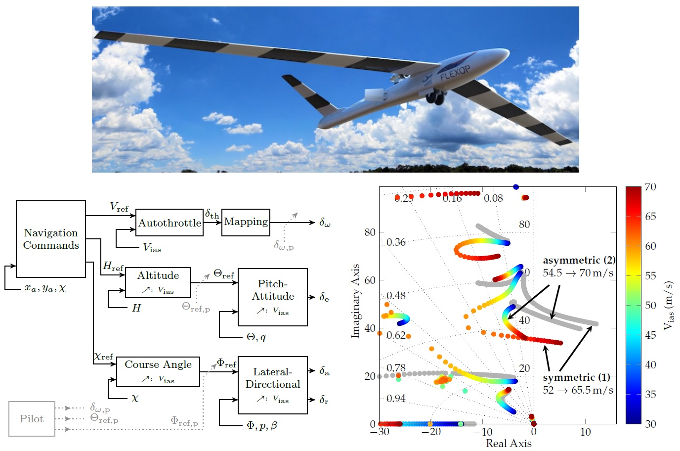
Section 3 are applied to the FLEXOP aircraft. The single-engined FLEXOP flutter demonstrator features a wing span of 7 m and is illustrated in
Figure 1. The takeoff weight is typically 55 kg but can be increased by up to 11 kg of ballast. Two wing-sets are designed and manufactured for the aircraft. The first one features a rigid structure with a flutter speed far beyond the operational aircraft velocity. This wing-set is mainly used for basic flight testing and rigid model verification. The second wing-set, which is considered in the models in this article, is flexible and has two main flutter modes within the operational velocity range.
The rigid body motion of this aircraft is described by a standard nonlinear six-degrees-of-freedom flight mechanics model (e.g., [
19]) in terms of translational velocities
u,
v,
w and angular velocities
p (roll),
q (pitch),
r (yaw) in the body-fixed frame. Orientation in the earth-fixed reference frame is described in terms of Euler angles
(bank),
(pitch), and
(heading). The angles between body-fixed frame and wind axes are angle of attack
and side-slip angle
. The flight path is described with respect to earth by the path angle
and the course angle
. To describe the flutter phenomena, the structural dynamics from a reduced finite element model are coupled with aerodynamics derived via the doublet lattice method. This coupling to derive the aeroelastic model is achieved via splining. For the flexible wing-set the first flutter mode (symmetric), becomes unstable at around 52 m/s with 8 Hz, while the second one (asymmetric) mode, follows at 54.5 m/s with 7.3 Hz [
11,
20]. A detailed description of the aircraft modeling and its analysis is also provided in [
10,
21].
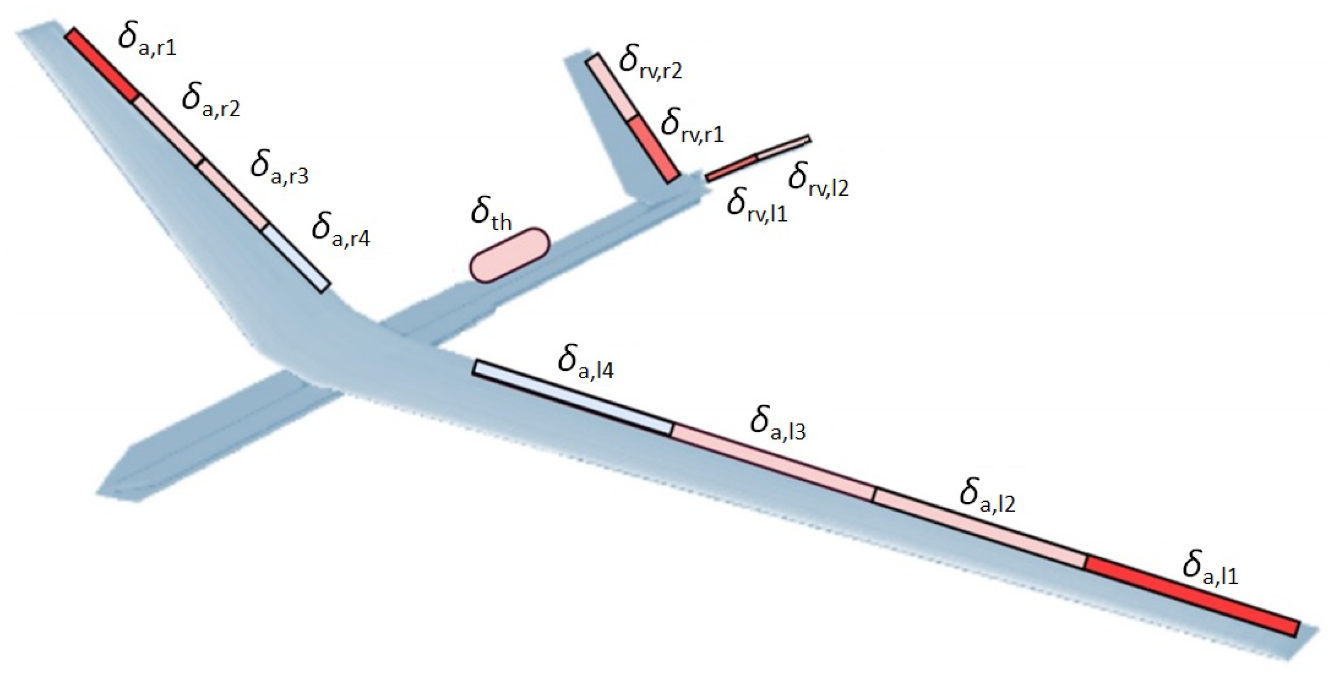
As control inputs the aircraft features four ruddervators on the aircraft’s V-tail, two on the left (
,
) and two on the right side (
,
) as illustrated in
Figure 3. These ruddervators combine the functionalities of classical rudders and elevators. The symmetric deflections of the ruddervator correspond to classical elevator deflections, while asymmetric deflections exhibit rudder deflections. Additionally, the aircraft has four pairs of ailerons. The most outer pair (
,
) is used for flutter control while the most inner pair (
,
) is used as high lift devices during takeoff and landing. The inner two pairs (
,
,
,
) are used in the baseline control law to control the aircraft’s roll motion. This rigorous dedication of each aileron pair to a single task is taken to simplify the control design tasks and avoid superposition of baseline and flutter control signals in the actuator commands during aircraft operation. The latter could result in actuator saturation which needs to be absolutely avoided to ensure stabilization of the flutter modes.
The actuators to steer the control surfaces are modeled as second order systems with rate and position limits to realistically reflect the actuator behavior. These models have been obtained through frequency-based system identification and data gathered on the various servos. The sensors of the aircraft are modeled as first order linear models including time delays. The aircraft is equipped with a 300 N jet engine [
22], located on the fuselage dorsal surface. A high fidelity, non-linear simulation model of the engine is available. Consequently, a simplified, control-oriented model has been developed and is considered in the controller design tasks. It features a dominant time delay of
s, a non-linear mapping from the engine’s revolution-speed to thrust (and versa), and a rather slow second-order dynamic. In addition, a velocity dependent saturation limit is considered. It describes how the available thrust decreases with increased inflow speeds.
4.1. Baseline Controller
Three different modes to control the aircraft are considered in the flight control system. These modes facilitate a stepwise augmentation of the aircraft during the flight test campaign:
- (i)
Direct Mode: The direct mode allows the pilot on the ground to bypass the flight control system. The only part active in the flight control computer is the mapping from the received remote-control signals to the commanded surface deflections. The pilot controls the pitch, roll and yaw axis directly via the aircraft’s control surface deflections and its velocity via the thrust setting.
- (ii)
Augmented Mode: The augmented mode switches on basic augmentation for the pilot [
23]. Instead of directly controlling the surfaces the pilot inputs pitch- and roll-attitude commands. The side-slip angle is automatically regulated to zero, reducing the pilots need to control the yaw axis separately. Velocity control remains in direct control, i.e., the pilot controls the velocity via the thrust setting.
- (iii)
Autopilot Mode: In this mode the pilot fully delegates the aircraft control to the flight control system. Altitude, course angle, velocity and side-slip angle are automatically controlled. To fly along the defined test pattern, reference commands based on the aircraft position are generated in a navigation module.
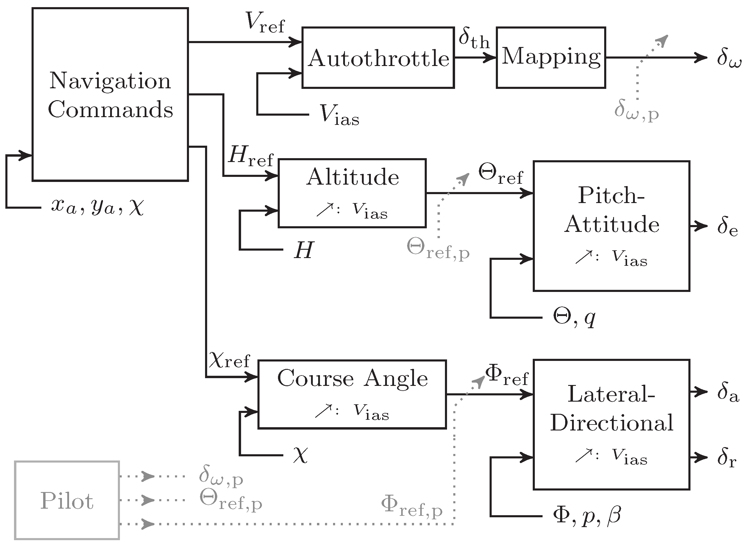
The inner loops of the control system in roll, pitch and yaw provide the basis for the operational model (ii) and (iii). Mode (iii) is the core element of the autopilot adding the outer loops for course angle, altitude and speed control (autothrottle) as illustrated in
Figure 4. Thus, a series of cascaded control loops is used to facilitate the control design task. As the cross-coupling between longitudinal and lateral axis is negligible, longitudinal and lateral control design is separated. Thrust commands
which are transferred to an engine revolution command
via a nonlinear mapping and the elevator
are the available actuators for longitudinal control. The available bandwidths for throttle and elevator differ considerably such that a combined control design does not promise any advantages. Thus, the reference
for the indicated airspeed
is controlled solely by the use of the throttle command
. The elevator command
is used to control the attitude in the inner loop and the vertical position of the aircraft in the outer loop. The pitch-attitude controller in the most inner feedback loop tracks the pitch-attitude (
), attenuates wind disturbances, and improves short period damping with the pitch rate (
q) measurement as an auxiliary feedback signal. The cascaded outer loop establishes control of the altitude (
H). Both controllers are scheduled with velocity (
), indicated by ↗ in
Figure 4, to achieve optimal performance over the required velocity range.
Lateral-directional control generates aileron (
) and rudder commands (
). The lateral-directional control problem is necessarily multivariable and requires the coordinated use of aileron command
and rudder command
. The most inner loop features roll-attitude (
) tracking, roll-damping augmentation via the roll rate (
p), and coordinated turn capabilities, i.e., turns without side-slip, via feedback of the side-slip angle (
). The outer loop establishes control of the course angle (
). Again, all controllers are scheduled with velocity to increase performance over the velocity range. Within the fully automated flight mode (iii) the reference signals for the velocity (
), altitude (
), and course angle (
) are provided by a dedicated navigation algorithm. It uses the GPS longitudinal and lateral position of the aircraft (
and
) as well as the current course angle (
) to provide the commands. More details on the algorithm are found in [
24].
The control loops use scheduled elements of proportional-integral-derivative (PID) controller structures with additional roll-offs in the inner loops to ensure that no aeroelastic mode is excited by the baseline controller. Scheduling with indicated airspeed
is used to ensure an adequate performance over the velocity range from 32 m/s to 70 m/s. For the scheduling a first or second order polynomial in
following Equation (
16) is applied. As an example, the proportional gain
depends quadratically on
with the free parameters
,
, and
. These free parameters are directly included in the optimization problem (
15). A comprehensive summary of the used controller structures for each cascaded loop is provided in
Table 1, including the channel description in the controller architecture and the implemented scheduling.
Please note that these controller outputs
,
, and
deffer from the actual surface inputs to ease the actual control design task. Thus, they need to be transformed to physical actuator commands via an adequate control allocation. The FLEXOP aircraft has multiple control surfaces and features combined rudder and elevator surfaces (ruddervators) as depicted in
Figure 3. The commands to the actuators of the two aileron pairs are determined by
to generate the required differential aileron deflections for roll motion control. For the ruddervators superposition of the elevator command
and the rudder command
is applied by
Thus, symmetric deflections on the left and right of the ruddervators correspond to elevator commands while differential deflections establish rudder commands.
Parameter Tuning
With the baseline controller structure available, the next step is to tune the free parameters of the individual control loops. Following the ideas of the model-based approach presented in
Section 3, an individual optimization problem is set up for the tuning of each control loop. The aircraft model used for the baseline controller design has the form (
12) and (
13) and represents the aircraft with the rigid wing-set. This model is substantially less complex than the model with the flexible wing-set. However, as the rigid body modes are barely changing with the wing-set, the baseline controller is used for both wing-sets. To not interfere with the flutter controller or excite flutter modes when using the flexible wing-set, adequate roll-off filter are included in the the design. Six optimization problems are deified for the baseline controller design problem, which are summarized in
Table 2. Please note that the proportional damping augmentations in roll and pitch are not tuned separately but included in the optimization problems of the corresponding tracking loops. For the inner loops a phase margin of at least 45
is demanded. As short period damping is relevant, a minimum of 0.6 is set as an optimization constraint. For the roll motion a fast response time of 1 s with good tracking capabilities (steady state error of 0.1) is defined. For the coordinated turn capabilities via the side slip angle feedback a single constraint on the disturbance rejection gain is applied.
For the outer loops, an adequate frequency separation is commonly required within the cascade controller design. The bandwidth of each cascaded loop is constrained by the lower-level control loops with the ultimate constraints being the servo actuator bandwidths. While the available servo actuators on the FLEXOP aircraft provide a sufficiently high bandwidth for the inner loop designs, the inner and outer loops need to be frequency separated from each other. Thus, the bandwidth design constrains for the outer loop are set to be five times lower than the bandwidths of their according inner loops. Finally, the auto-throttle is a little more involved due to the complex engine dynamics. Therefore, a model matching problem using the non-linear simulator is used which aims to minimize the recorded error between the desired and achieved response in the simulation. More details on the tuning are provided in [
24].
4.2. Flutter Suppression Controller
The two flutter modes mainly limiting the operational velocity range of the aircraft with the flexible wing-set are well distinguishable by their symmetric and asymmetric mode shapes. Both modes describe a dynamic coupling of the wing bending and torsion which becomes unstable above certain airspeeds. To individually stabilize the two flutter modes, the
-optimal blending approach proposed in
Section 2 is applied to the FLEXOP demonstrator. In doing so, the flutter modes are decoupled which allows for a straight forward design of two dedicated SISO control loops, one for each flutter mode.
4.2.1. Input-Output Blending
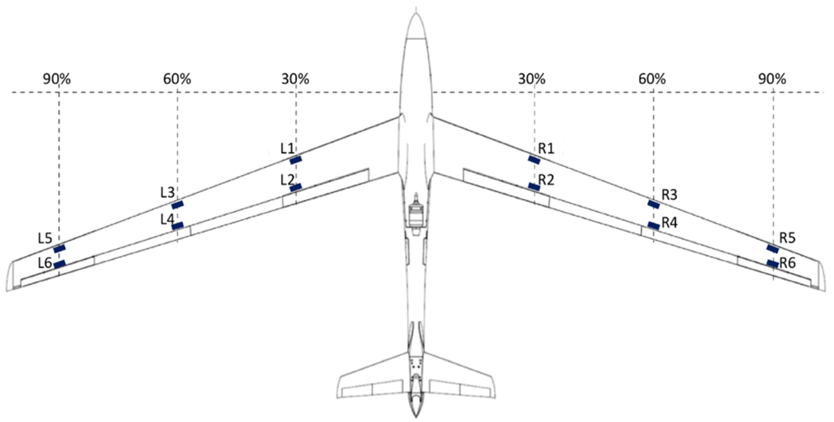
The measurement signals considered for flutter suppression are captured by the inertia measurement units (IMUs) located in the wings and in the center of gravity, where only vertical acceleration and pitch rate measurements are used for the controller design herein. In
Figure 5, the location of the IMUs in the wings together with the location of the ailerons, of which only the outer pair is used for flutter suppression.
Before actually blending the given inputs and outputs, it is proposed to normalize the rate and acceleration measurements since they are of different units, see [
13] for more details. Subsequently, the
-optimal blending vectors associated with the first (symmetric) and second (asymmetric) flutter mode are computed according to
Section 2.2. The obtained input and output blending vectors basically mirror the shape of the underlying modes and hence are also symmetric and asymmetric. Furthermore, sensors at the outer part of the wing are better suited to measure the corresponding flutter modes and hence are higher weighted in the output blending vector. Since the mode shapes change only slightly within the critical airspeed range, it is sufficient to compute the blending vectors at a single airspeed
and hold them constant within the whole flight envelope.
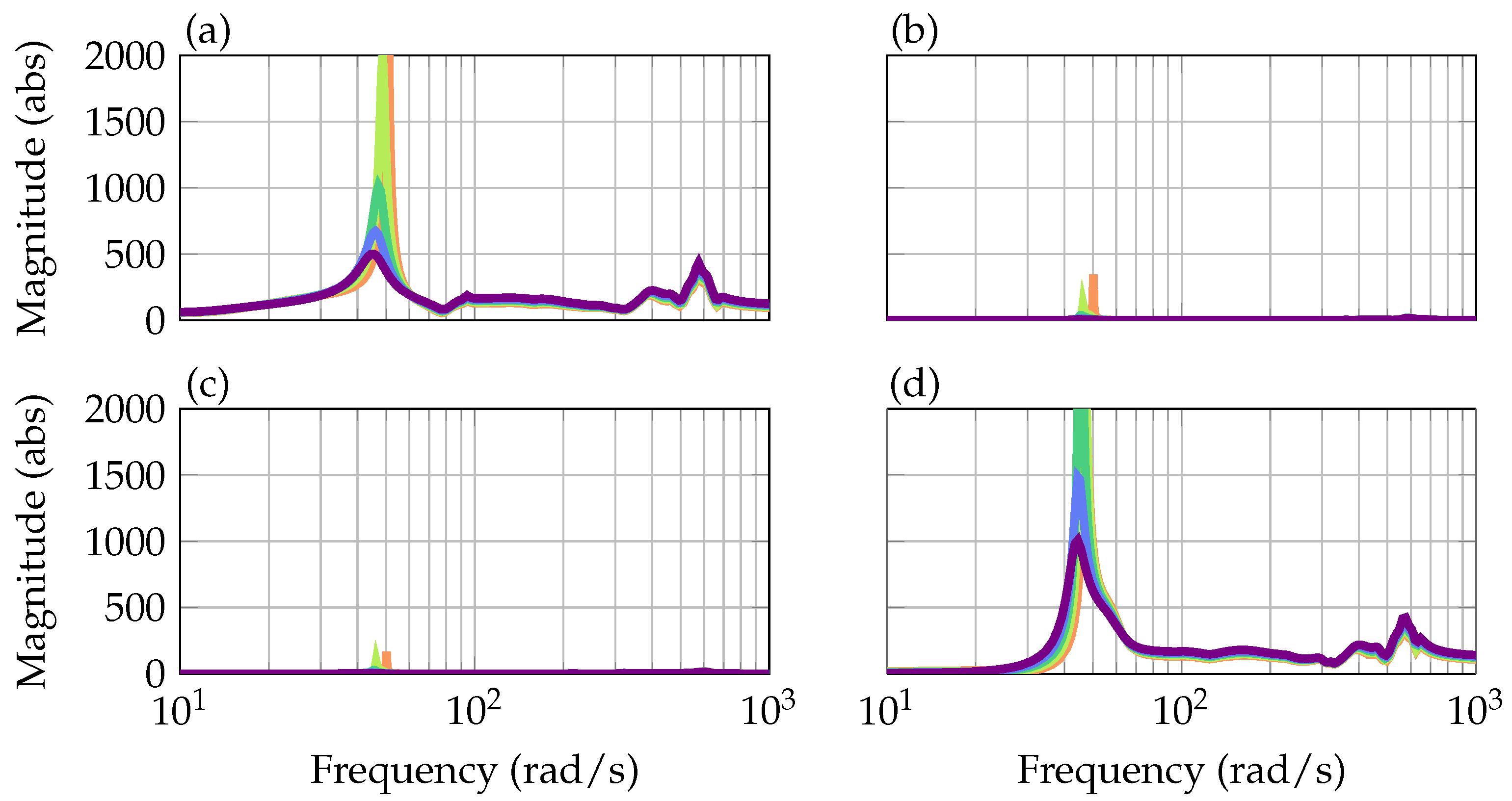
As illustrated in
Figure 6, the two flutter modes are well decoupled by the determined blending vectors. The virtual inputs and outputs of both flutter modes do not interfere with each other which is indicated by the negligible small magnitude on the top right and bottom left graph in
Figure 6. Furthermore, the blended inputs and outputs clearly emphasize the individual flutter modes while the contribution of other nearby aeroelastic modes is minor. Taking a look at the higher frequency range, however, it has to be noticed that the flutter modes are not fully decoupled from the rest of the system. This is counteracted efficiently by adding a low pass filter due to the large frequency separation as described in the following subsection.
4.2.2. Single-Input Single-Output Controllers
With the derived blending vectors it is possible to design dedicated SISO controllers for the symmetric (
) and asymmetric (
) flutter mode. The structure of the SISO controllers is predefined as
where
denotes a bandpass filter to ensure that no interference with the baseline controller occurs and higher frequent modes are not excited. For both flutter modes, a second order Butterworth filter is chosen with a fixed passband from 40
/
to 400
/
. The corresponding corner frequencies are selected such that both flutter modes are well inside the passband and controller performance is affected as little as possible. Since a large velocity range needs to be considered, the core of the flutter suppression controller
is gain-scheduled. For better tuning capabilities, it is desired to keep the order of
as small as possible while a larger order may allow for a better controller performance. Hence, a careful balancing between controller order and performance is required. For the first (symmetric) and second (asymmetric) flutter mode, an order of two respectively one is chosen. The state space matrices
of
depend linearly on the indicated airspeed, i.e.,
, where the matrices
and
are subject to be optimized. The two optimization problems to design the two SISO controllers have the form (
15). As explicit optimization criteria a gain margin of 6 dB and a phase margin of 45
are demanded in the optimization. The two problems are again solved using non-smooth optimization techniques [
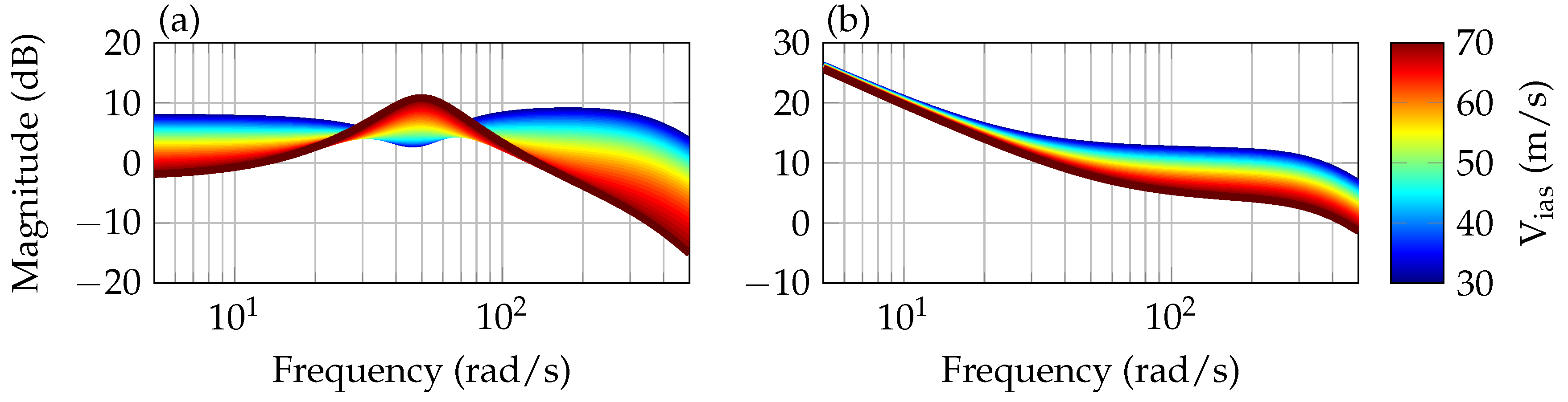
18]. The resulting SISO controllers without the band-pass filter are depicted in
Figure 7. Please note that with increasing airspeed, the controller gain increases in the symmetric case and decreases in the asymmetric case in the frequency range of the corresponding flutter mode.
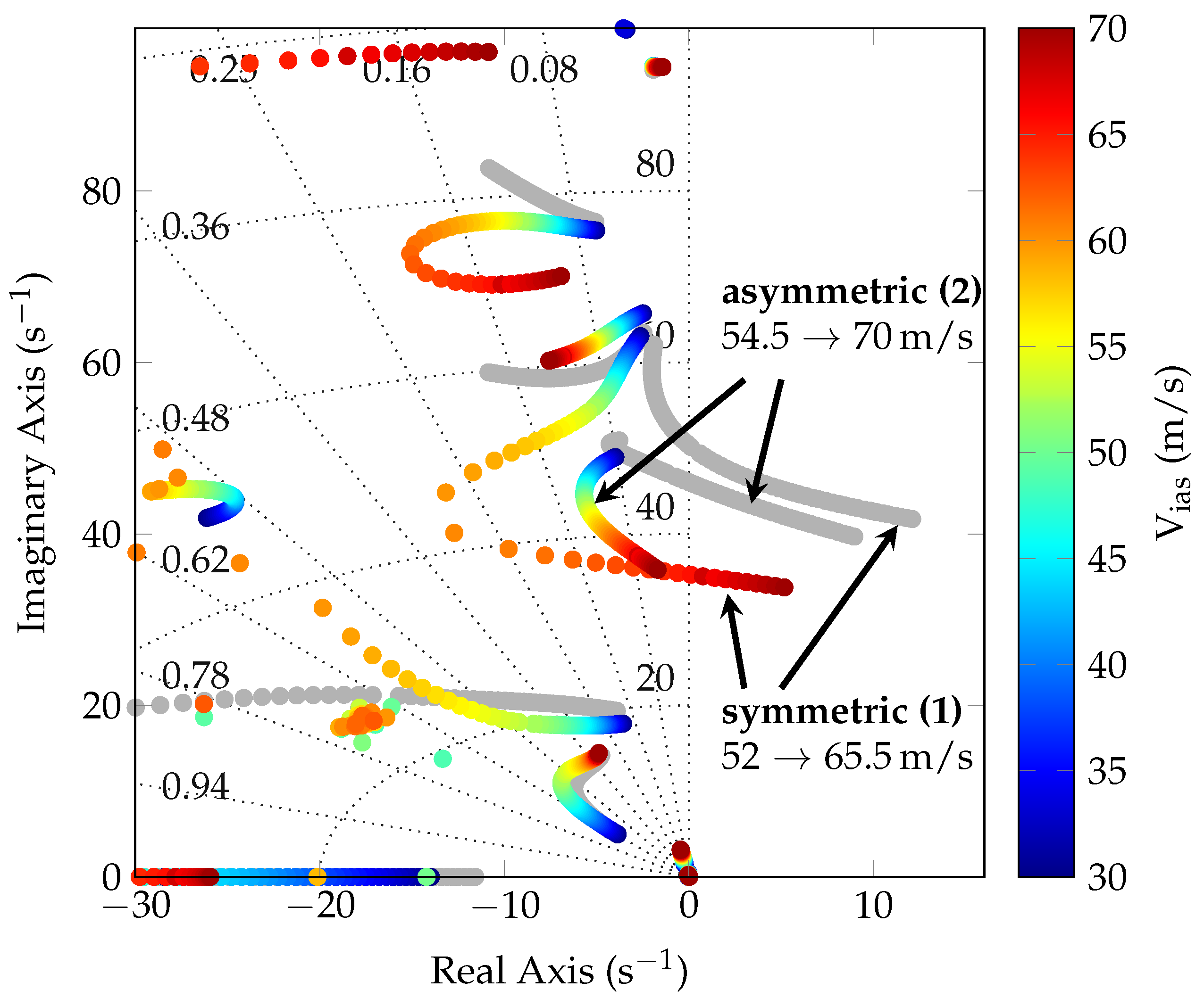
Closing the two SISO loops stabilizes the two flutter modes as it is illustrated in the pole migration plot in
Figure 8. The plot compares the closed loop poles of the aircraft with the baseline controller depicted in gray to the closed-loop poles of the aircraft with baseline and flutter controller depicted in color in dependence of the airspeed. Clearly visible is the unstable behavior, i.e., the crossing to the right half plain of the first (symmetric) and second (asymmetric) flutter mode in the open-loop. With the flutter suppression controller the symmetric flutter mode is stabilized up to airspeeds of 65.5 m/s. The asymmetric mode is stabilized even beyond 70 m/s. Demanding additional single-loop robustness margins of 6 dB in gain and 45
in phase to the critical point, leads to a maximum operational speed of about 60 m/s. This still results in an increase in allowable speed of more than 15 % compared to the case without active flutter suppression. Also noticeable is that the other poles of the system(s) are not largely affected by the flutter suppression controller. This is acceptable since damping is increased rather than decreased.
The linear analysis results discussed in this section provide an initial verification of the controller. The next mandatory step on the way to the implementation of the control algorithms on the aircraft is to test them in a non-linear simulation environment of the aircraft to gather further insight into the performance and robustness of the developed algorithms.
5. Verification
The developed flight control system including the basic augmentation to autonomously fly the aircraft and the flutter control algorithm are verified in a non-linear simulator and a summary of the important results is provided in this section. The baseline controller shall work for both wing-set configurations, i.e., the rigid and the elastic one. A detailed description of the baseline control architecture and a coherent analysis with the rigid wing set is provided in [
24]. The advancement herein is to fly the aircraft with the flexible wing set beyond the flutter speeds of approximately 52 m/s and 54 m/s. Thus, the findings from the linear analysis in
Section 4 which indicate an extension of the flutter phenomena from 54 m/s to 66 m/s for the asymmetric flutter mode and from 52 m/s to 70 m/s for the symmetric flutter mode are verified. Therefore, a simulation-based verification using the developed high fidelity simulator presented in [
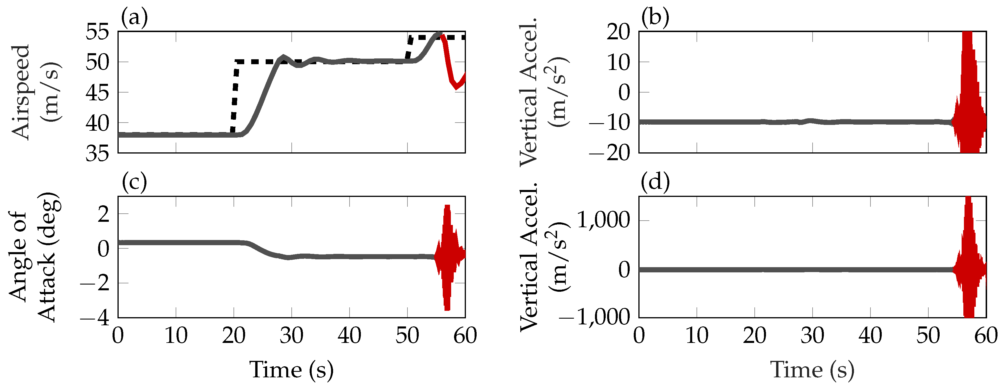
10] is performed. To provide some insight in the open-loops flutter behavior, i.e., without active flutter control, the aircraft is accelerated from its trim condition at 38 m/s to 50 m/s. From there on the speed is increased by 4 m/s to enter the flutter region.
Figure 9 depicts the aircraft speed in the diagram (a), the vertical accelerations on the wing root of the left wing in diagram (b), the aircraft’s angle of attack in diagram (c), and the vertical accelerations on the left wing tip in diagram (d). The first step in the reference airspeed happens at 20 s simulation time. The aircraft accelerates, leading to a reduction of the required angle of attack (c) to hold the altitude, and reaches the commanded speed of 50 m/s. At 50 s simulation time the reference speed is increased by 4 m/s. The aircraft reaches the flutter speed and the wings start to oscillate, indicated in red (
![Aerospace 06 00027 i001]()
) in the diagrams of
Figure 9. This leads to high accelerations on the wings, which is depicted in the diagrams (b) for the left wing root and in diagram (d) for the left wing tip. In reality, the aircraft would have been lost at this point, but the resulting non-linear behavior is not covered by the simulation.
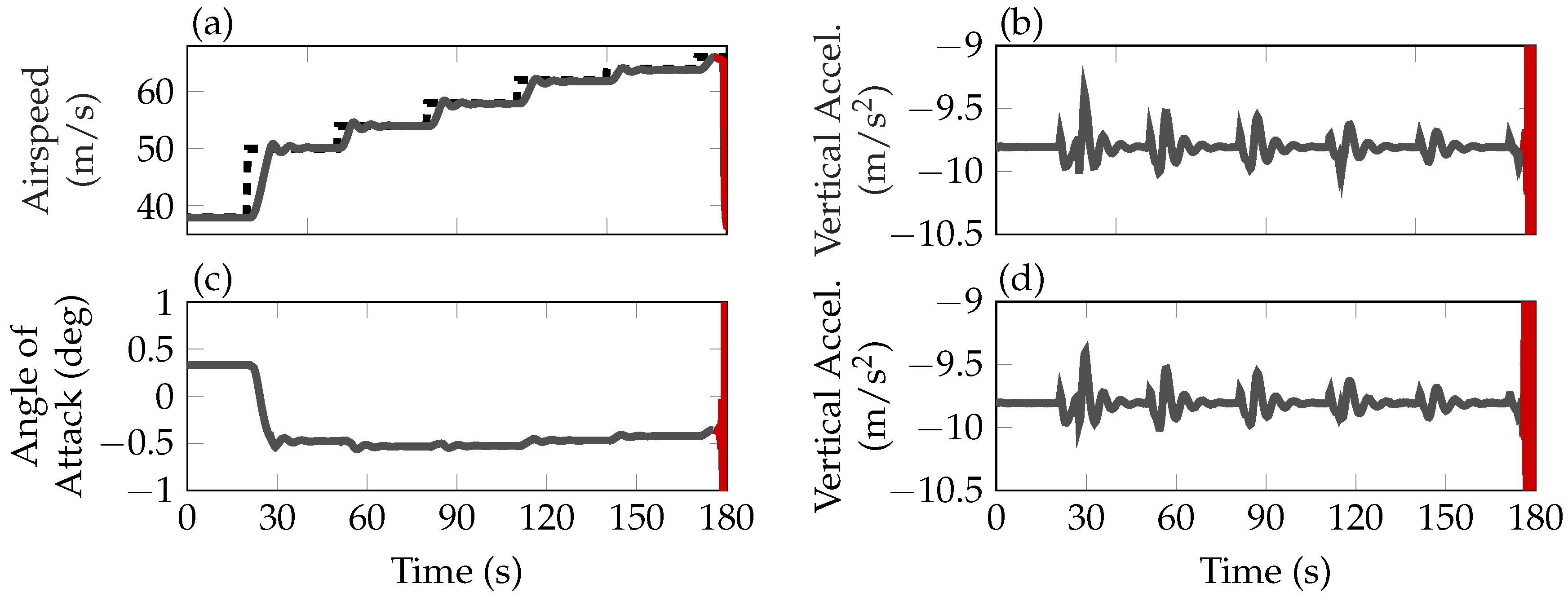
In
Figure 10 the same scenario is simulated with the flutter suppression controller enabled. The velocity. depicted in diagram (a), is increased step-wise until flutter occurs. The aircraft is stabilized up to an indicated airspeed of about 65 m/s, as predicted by the linear analysis. The accelerations on the wing, depicted in diagrams (b) and (d), are kept close to their trim conditions by the flutter suppression controller. After initiating the velocity step from 64 m/s to 66 m/s the first symmetric flutter mode becomes unstable. This instability is indicated in the diagrams of
Figure 10 by the changing the line color to red.
Next, the aircraft is simulated on the predefined flight test pattern. For the description of the pattern it is assumed, without loss of generality, that the north direction is equal to the
y-axis of the defined coordinate system. The main waypoint to be tracked is chosen before the turn of the actual flutter test. Thus, the inbound leg is dedicated to the waypoint tracking to ensure a uniform start of the outbound turn. After the outbound turn the aircraft reaches the outbound leg, on which the aircraft velocity is increased to test the active flutter control. On the last part of the outbound leg the aircraft is decelerated to avoid flying the turns above the open-loop flutter speed. Overall, this results in four main segments, for which the reference signals need to be provided. To generate the reference signals a state-machine with sub-tasks, which are selected based on switching criteria, is implemented. This state-machine together with the presented baseline and flutter suppression controller allow navigating the aircraft around the test pattern fully autonomously. In
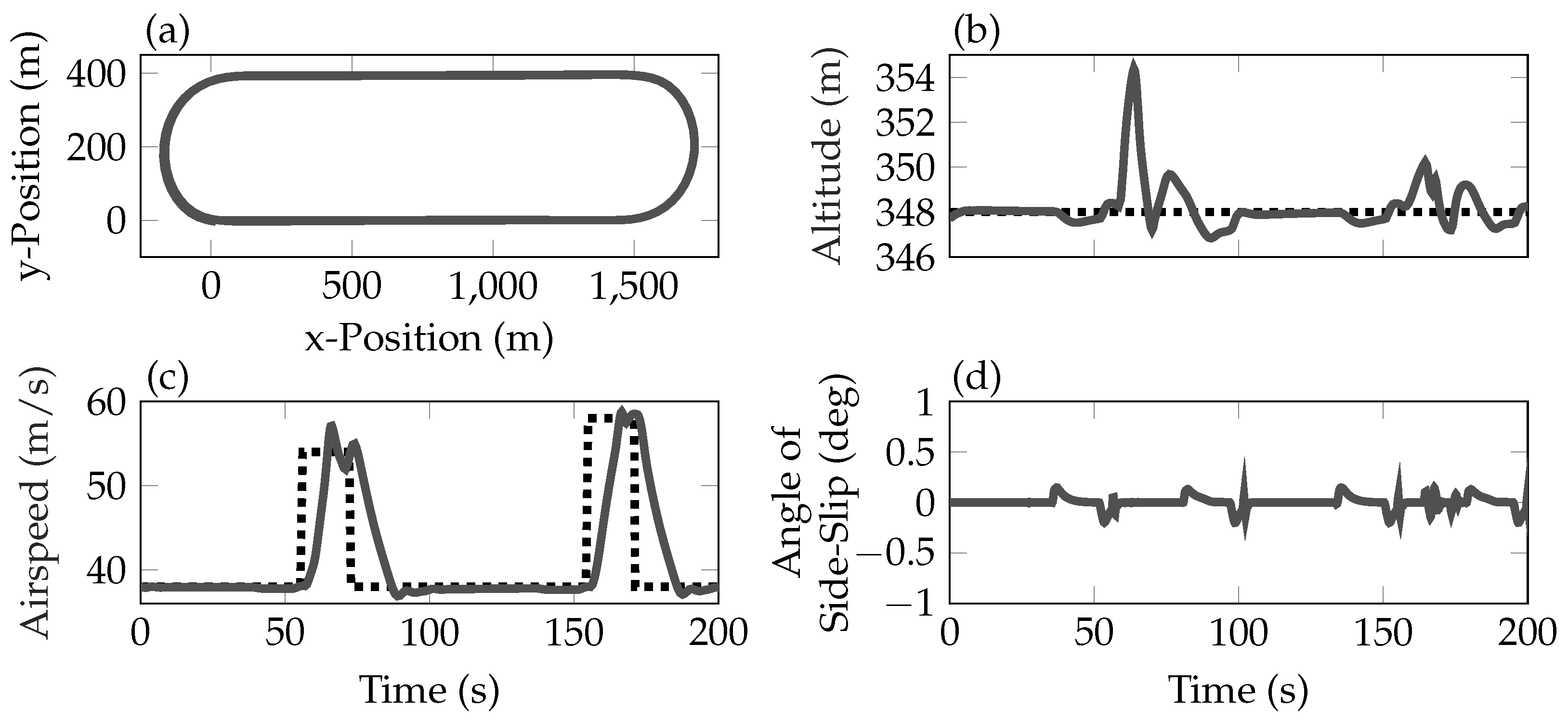
Figure 11 relevant flight parameters during a simulated flight of 200 s along the described test pattern is depicted. In diagram (a) the longitudinal and lateral position of the aircraft is shown. The 200 s flight time correspond to approximately two laps on the pattern. On the test leg of each lap the aircraft is brought into the open-loop flutter regime. The indicated airspeed (
![Aerospace 06 00027 i002]()
) is depicted in diagram (c) together with it reference command (
![Aerospace 06 00027 i003]()
). The pattern is flown with a nominal speed of 38 m/s. On the test leg the speed is increased to 54 m/s in the first lap and 58 m/s in the second lap. The altitude is maintained by the control system at 348 m shown in diagram (b). The visible spikes at about 65 s and 160 s in the altitude and airspeed are due to vertical wind gusts simulated on the test leg to verify the control system’s robustness against disturbances. The control system maintains the angle of side-slip around zero during the whole flight including the turn maneuvers. Thus, the baseline controller is able to adequately track the demanded values in the relevant flight parameters.
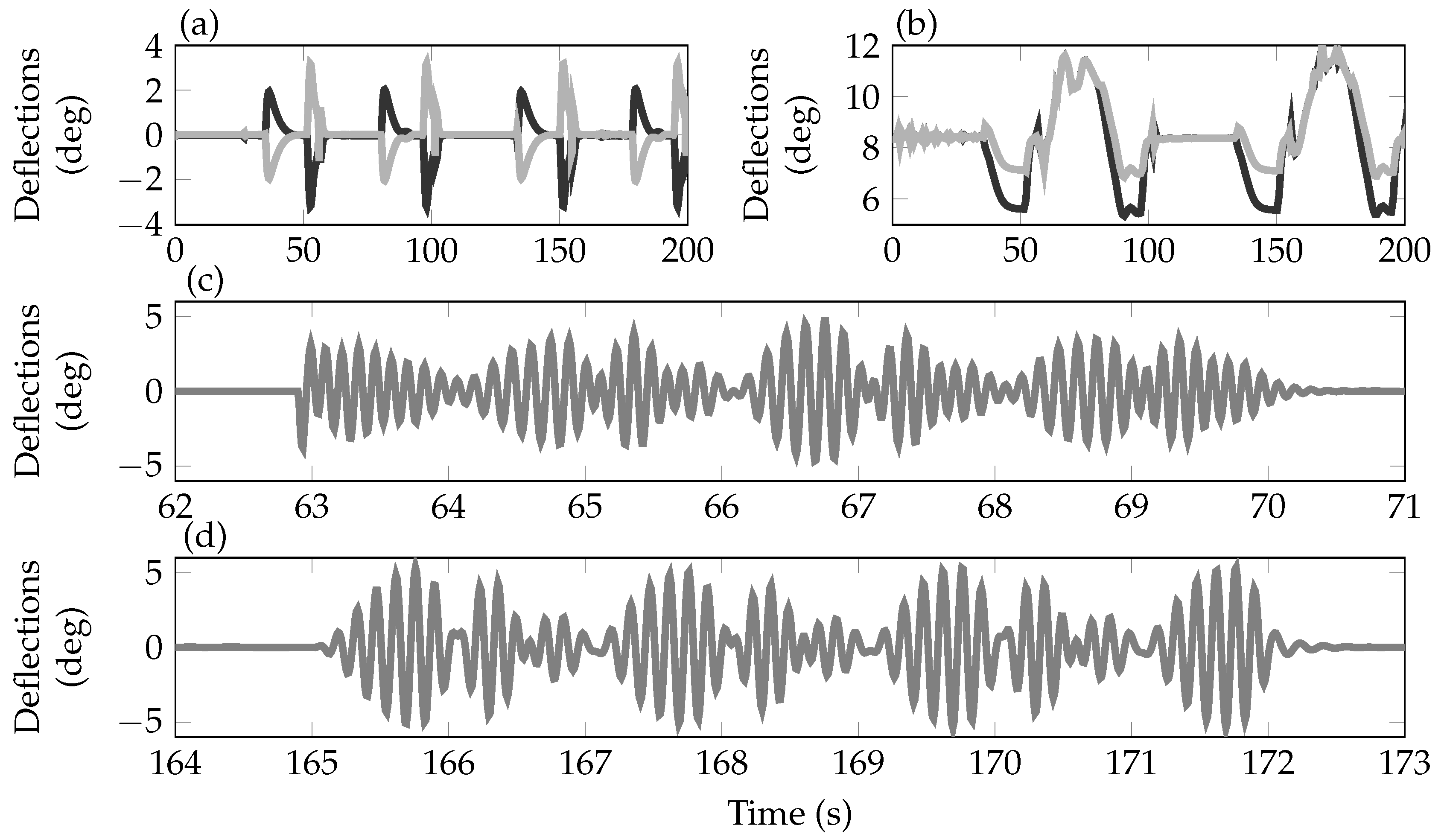
In
Figure 12 the corresponding control surface deflections of the ailerons and the ruddervators are depicted. In diagram (a) the deflections of the two left (
,
) and the two right (
,
) aileron pairs used to control the roll motion of the aircraft are shown. Due to selected aileron control allocation described in Equaiton (
17), the deflections are identical for the two left and two right ailerons, respectively.
A moderate deflection of
3
is necessary to bring the aircraft to the desired bank angle of 45
during the turns and back to 0
after the turns. In diagram (b) the deflections of the ruddervators are shown, which are the result of the superposition of the rudder and elevator commands from the baseline controller, following from the control ruddervator allocation in Equaiton (
18). Again, the deflections on each side are identical so that only two lines are visible. The deflections of about ± 45
around the trim value of ≈ 8
required to ensure the coordinated turn without side slip angle (
) and to track the reference altitude during the turns and on the test leg. Diagram (c) depicts the deflections of the outer aileron pair (
,
) between 62 s and 71 s simulation time, i.e., when the aircraft is flown within the open-loop flutter regime. The depicted deflections are required to stabilize the aircraft. Only a single line is visible as in the velocity range up to 58 m/s the symmetric flutter mode is the predominant, unstable mode. Diagram (d) depicts the deflections of the outer aileron pair between 164 s and 173 s simulation time, i.e., when the aircraft is accelerated to 58 m/s reference speed. The required deflections for stabilizing the aircraft are comparable to the ones at 54 m/s airspeed.
Figure 13 depicts the resulting accelerations on the tip of the left wing in the vertical direction (
![Aerospace 06 00027 i004]()
) and horizontal direction (
![Aerospace 06 00027 i005]()
), where the latter is directed into the flying direction. The flutter suppression controller is able to stabilize both flutter modes during the whole test, leading to deviations of
m/s
from the trim point for the vertical accelerations and
m/s
for the horizontal accelerations. To summarize the performed verification campaign, the developed control system including the baseline and flutter suppression controllers is able to satisfactorily navigate along the defined flight test pattern and stabilize the flutter as predicted with the linear analysis also in wind scenarios. These results provide confidence that the developed system will also work satisfactorily during the real flight tests.


 ) in the diagrams of Figure 9. This leads to high accelerations on the wings, which is depicted in the diagrams (b) for the left wing root and in diagram (d) for the left wing tip. In reality, the aircraft would have been lost at this point, but the resulting non-linear behavior is not covered by the simulation.
 ) is depicted in diagram (c) together with it reference command (
  ). The pattern is flown with a nominal speed of 38 m/s. On the test leg the speed is increased to 54 m/s in the first lap and 58 m/s in the second lap. The altitude is maintained by the control system at 348 m shown in diagram (b). The visible spikes at about 65 s and 160 s in the altitude and airspeed are due to vertical wind gusts simulated on the test leg to verify the control system’s robustness against disturbances. The control system maintains the angle of side-slip around zero during the whole flight including the turn maneuvers. Thus, the baseline controller is able to adequately track the demanded values in the relevant flight parameters.
 ) and horizontal direction (
  ), where the latter is directed into the flying direction. The flutter suppression controller is able to stabilize both flutter modes during the whole test, leading to deviations of m/s from the trim point for the vertical accelerations and m/s for the horizontal accelerations. To summarize the performed verification campaign, the developed control system including the baseline and flutter suppression controllers is able to satisfactorily navigate along the defined flight test pattern and stabilize the flutter as predicted with the linear analysis also in wind scenarios. These results provide confidence that the developed system will also work satisfactorily during the real flight tests.
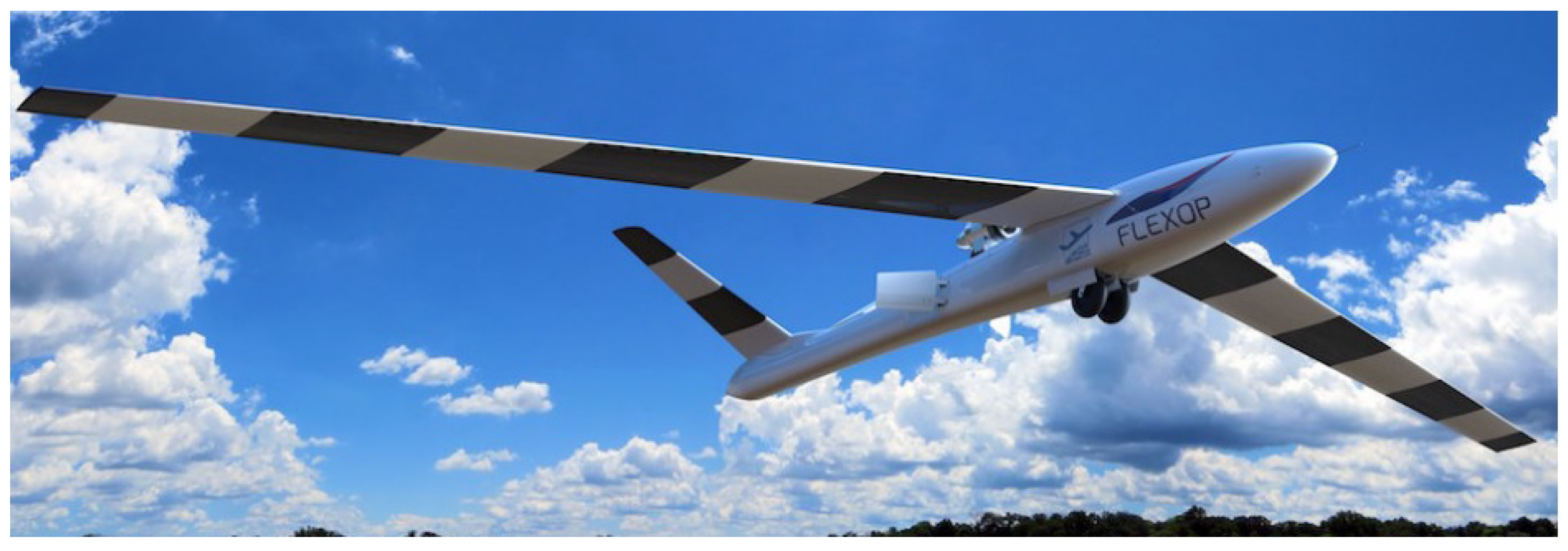

 ), 54 m/s (
  ), 56 m/s (
  ), 58 m/s (
  ), and 60 m/s (
  ) indicated airspeed .

 ), the unstable situation in red (
  ).
).
 ), the unstable situation in red (
  ).
).
 ) and horizontal (
  ) accelerations on the left wing tip.
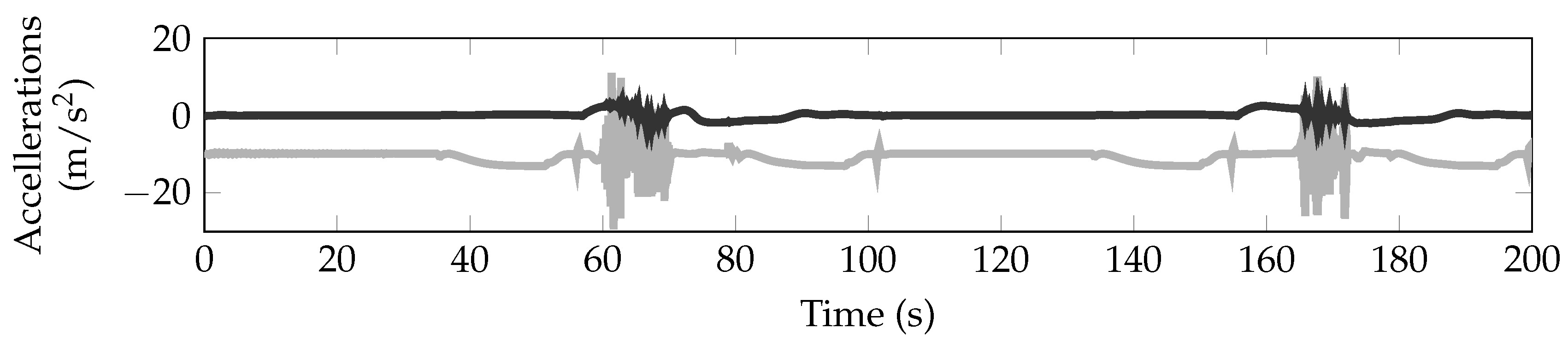
