Abstract
An extant bird resorts to flapping and running along its take-off run to generate lift and thrust in order to reach the minimum required wing velocity speed required for lift-off. This paper introduces the replication hypothesis that posits that the variation of lift relative to the thrust generated by the flapping wings of an extant bird, along its take-off run, replicates the variation of lift relative to the thrust by the flapping wings of a protobird as it evolves towards sustained flight. The replication hypothesis combines experimental data from extant birds with evidence from the paleontological record of protobirds to come up with a physics-based model of its evolution towards sustained flight while scaling down the time span from millions of years to a few seconds. A second hypothesis states that the vertical and horizontal forces acting on a protobird when it first encounters lift-off are in equilibrium as the protobird exerts its maximum available power for flapping, equaling its lift with its weight, and its thrust with its drag.
1. Introduction
Lift is often considered the primordial force leading the primitive, evolving bird, referred to here as a protobird, towards sustained flight, a pervasive concept in the field of flight biomechanics. A protobird is a non-flying, non-descript animal capable of running while generating thrust (and some “residual” lift) by flapping its wings. The limited flapping kinematics of a protobird is assumed to involve a low level of specific kinetic energy (per unit mass) available at its wings, that increases along evolution, until reaching a critical level. Further increase in its kinetic energy allows it to reach level flight (L = W) without the possibility of ascending flight, at which point, the flyer is referred to as a bird.
The use of the word “lift” may mislead one to the apparently foregone (and reasonable) conclusion that lift invariably lifts the protobird up during lift-off, resulting in spontaneous ascending flight. As a result, lift is frequently referred to as “fighting” gravity along the evolution to sustained flight [1,2]. Moreover, the mention of the words “flapping wing” brings to mind the word “lift”, but rarely the concept of “thrust”.
This paper presents: (i) the replication hypothesis, applicable along the take-off run of a protobird, and (ii) a hypothesis that proposes the protobird to be in equilibrium when first encountering lift-off, a condition defined by two simultaneous equations.
Both of these hypotheses make use of the normalized lift, ηL, normalized thrust, ηT and the normalized drag, ηD (counterparts to the lift coefficient CL, the thrust coefficient CT, and the drag coefficient, CD), nondimensional numbers that have a physical meaning, and can be applied directly to flapping wings without resorting to the blade element method [3]. A review of these normalized forces follows.
2. A Review of the Normalized Forces
The lift, thrust, and drag equations of flapping wings used in this paper are reviewed next by comparing the legacy vector scenario with the scalar scenario adopted in this paper.
The vector scenario: The velocities involved in the flow field surrounding a flapping wing, illustrated in Figure 1, limited to an instant t during its downstroke and at a particular spanwise station, are the translation (or forward) velocity, v∞, the flapping velocity, vf, and the resultant wing velocity, vw.
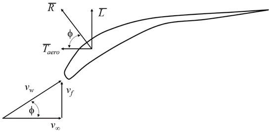
Figure 1.
The vector field at a given wing station “y” and at an instant t during the downstroke.
The lift L of a fixed translating wing of an aircraft during its take-off run or during cruise flight and the flapping wing of a flyer is, in both cases, perpendicular to the translation (or forward) velocity, v∞. The main difference between these two wings is that the wing of an aircraft, which has a fixed angle of incidence with respect to the fuselage, is able to generate only lift L, not thrust T. By contrast, the flapping wing has the ability to supinate (during the upstroke) and pronate (during the downstroke), allowing the airfoil to align itself to the incoming flow and is able to generate thrust T, Figure 1.
The wing velocity, vw, is the vector summation of the other two velocities:
It is seen that each of the above velocities vary with time t and wing span station “y” and, so, a double integral is in order when vw (actually vw2) is used for the calculation of the aerodynamic forces [2].
The “objective” (there are no objectives per se along evolution) behind a bird’s take-off run is to equal (in a protobird) or exceed (in a bird) the minimum wing velocity, vw min, at which point lift L equals (or exceeds) weight W, as the thrust T acts as the primordial force that allows the flyer to reach for this all-important velocity. In this vector scenario, the all-important wing velocity vw (which takes the role of the translation velocity, v∞, in the lift equation for fixed wings) is calculated by applying the labor-intensive blade element method.
The scalar scenario: The kinetic energy scenario is a more practical approach to calculating the average aerodynamic forces by flapping wings involving its translation velocity, v∞, and angular velocity, ω. The two relevant kinetic energies available at a flapping wing are shown in Figure 2 [4].
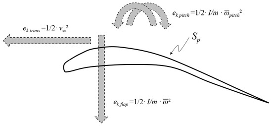
Figure 2.
Three sources of kinetic energy that are physically relevant throughout the evolution towards sustained flight, translation, flapping, and cyclic wing pitch (pronation–supination).
Note that the scalar scenario describes its relevant physics available at the complete wing, not at a given instant and spanwise station.
Borrowing a parameter from the scalar scenario, the legacy dynamic pressure, q∞, introduced by Prandtl circa 1921 [5], it can be used to quantify the specific kinetic energy due to the translational speed, multiplied by the density of the medium:
An expansion of this dynamic pressure allows for the algebraic addition of the kinetic energy due to flapping, ek flap, a function of the average angular velocity due to flapping, ω. This expansion is referred to as the kinetic pressure, Q∞ (from kinetic energy-based pressure):
The angular velocity ω in the above equation describes the kinetics involved in the continuous rotation of propeller blades and lift rotors [3], as well as the cyclic wing flapping of birds, bats, and insects [2], as used in this paper and defined numerically by Equation (9) below.
The equation for lift L, thrust T and drag D by flapping wings can now be written as an aerodynamic force F that equals the product of the kinetic pressure, Q∞, a normalized force ηF, (a counterpart to the lift, thrust and drag coefficients CL, CT, and CD), and the corresponding reference areas, Sref [3]:
The lift L of flapping wings of wing planform area, Sp, as Sref, translating at a velocity, v∞, and flapping at an average angular velocity is
The above equation is written as
According to Equation (1), the wing velocity, vw, equals
The specific moment of inertia I/m is the ratio of the wing’s moment of inertia I due to its mass distribution along its wing semispan r and the mass m of the “lifting system”, the protobird’s. Assuming the wing has a mass distribution along its wing length r similar to that of a cylindrical rod about its end, its specific moment of inertia I/m is [5]
The angular velocity ω of a flapping wing is a function of the flapping frequency f of the wing (the frequency of the upstroke and downstroke during flapping), in Hz, (f is equal to half the stroke frequency, fst) and the amplitude or stroke angle Ф in radians, the flapping angle of the wing over one flapping stroke [2]:
The wing velocity, vw, Equation (7), is rewritten next by replacing the specific moment of inertia, I/m, by (1/3·r2) from Equation (8), and the angular velocity ω by (2∙f∙Ф) from Equation (9):
Reorganizing terms, we obtain
The product Ф·r is the arc A subtended by the tip of the wing of half span r as it flaps at an amplitude angle Ф. This length multiplied by (2·f) results in the average tangential velocity vtt at the wing tip (the subscript tt stands for tip, tangential) during a flapping stroke. The average velocity of the wing, vw, is
The wing velocity vw is next written as a function of the Strouhal number, the ratio of the tangential velocity at the tip of the flapping wing, vtt, and its forward speed, v∞:
This definition of the wing velocity, vw, derived using the scalar scenario, varies slightly from Lentink and Dickinson’s definition of its characteristic speed, U, derived from the vector scenario [6].
The kinetic pressure Q∞ in Equation (3) is written as
The equation of lift L of flapping wings is
For a Strouhal number, St = 0, the above equation equals the legacy lift equation of a translating, non-flapping wing of a gliding bird or an aircraft, where the normalized lift, ηL, equals the lift coefficient, CL, and the reference area, Sp, its wing planform area.
The above format quantifies the thrust T of flapping wings:
Likewise, the drag equation can also be written as a function of the Strouhal number, St, but for simplicity, this paper assumes the drag D of a flapping flyer to be similar to its non-flapping counterpart ( = 0 St = 0), of frontal area, Sf:
This equation is similar to the legacy drag equation where the normalized drag, ηD, equals the drag coefficient, CD.
When the aerodynamic force vector ( or ) is positioned (close to) perpendicular to the respective reference areas Sref, ( ┴ Sp, ┴ Sf), the maximum value of the corresponding dimensionless number (ηL max, ηD max) is expected to be close to 1 (this does not apply to thrust as it is not found close to perpendicular to the reference area Sp of a flapping wing, Figure 1). Notwithstanding the fact that the values of ηL max and ηD max are dependent on Reynolds numbers, the fact that these nondimensional numbers are close to 1 (i) allows them to be used as figures of merit for the comparison of dissimilar lifting systems (like comparing flapping wings and rotating cylinders in Magnus effect in the same footing), (ii) allows them to be estimated when their values are unknown, and (iii) allows them to be interpreted as the ratio of specific work, w, and specific kinetic energy, ek [3]:
The reference area Sref for normalizing lift L and drag D are thus selected as the wing planform area, Sp, and the frontal area, Sf, respectively. The reference area for normalizing thrust T is the wing planform area, Sp.
3. A First Hypothesis: The Replication Hypothesis along the Take-Off Run
For discussion purposes, a bird is defined as a flapping flyer capable of ascending (oblique or vertical) flight after reaching lift-off (L > W) and a protobird is a flapping flyer not capable of ascending flight following lift-off due to insufficient flapping power available, a condition referred to as level lift-off (L = W). An analogous protobird has similar weight, wing loading and wing velocity vw as a bird, as evidenced from its paleontological record. Although both a bird and an analogous protobird are involved in this hypothesis, it is not implied that one evolved from the other.
The replication hypothesis posits that the variation of lift relative to the thrust generated by the flapping wings by a bird along its take-off run closely replicates the variation of the lift relative to the thrust by an analogous protobird along its evolution. This hypothesis scales a process lasting millions of years to one lasting few seconds in an analogous way a wind tunnel test scales down the large size of an aircraft to a more manageable wind tunnel model. The replication hypothesis does not require any Reynolds number corrections.
The lift and thrust vectors generated by flapping wings along the take-off run and averaged over time are perpendicular to each other, Figure 1, and so the magnitude of the resultant vector is
The angle of the resultant with the horizon is referred to as the lift activity angle, θ:
The lift activity angle θ along the take-off run may vary from approximately 10° to 90°, and is a measure of the ability by flapping wings to generate a lift L, relative to the thrust T. Its progression as it applies to both bird and protobird is reviewed next by segmenting their take-off run from stand-still to lift-off in three stages.
Thrust-predominant Stage I: This stage is characterized by the prevalence of thrust T over lift L, most of it generated by friction between the soles of its feet and the ground or by paddling over water, Trun, and supplemented by the thrust due to flapping, Taero:
The aerodynamic thrust Taero is generated by the protobird’s mechanism of pitch cycling about the spanwise axis of the wing, a wing’s aeroelastic response to flapping in the form of a cyclic pronation and supination of the wing. The low kinetic energy cost of this pitch cycling process may have facilitated the role of thrust T as the primordial force along the protobird’s evolution. More on this subject in Section 4.2.
Throughout this first stage, lift L plays a residual role on the flyer, and is illustrated by the flapping and paddling puffin, Figure 3, which finds its lift activity angle θ to be within a range of, say, 10° and 35°.
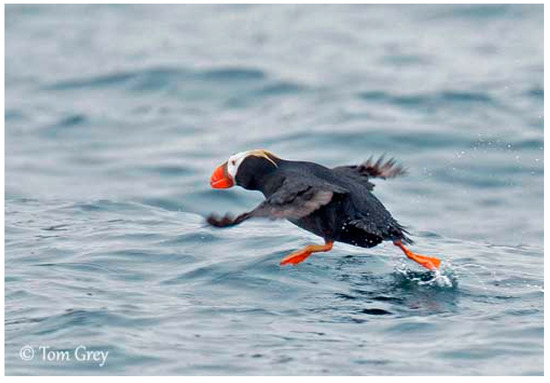
Figure 3.
The puffin during stage I of the take-off run, where thrust T has a dominant role over lift L [7].
Thrust & Lift-shared Stage II: This second stage finds the lift activity angle, θ, varying between 35° and 50°, where lift shares similar values with thrust T, and a resulting gradual decrease in the generation of Trun due to the increase in lift that reduces the normal force between the soles of the flyer and the ground, as Trun equals:
At a lift activity angle θ of 45°, the thrust T equals the lift L. This condition, a symbolic milestone referred to as the thrust-to-lift crossover, has no discerning dynamic effects on the bird or protobird.
Lift-predominant Stage III: The lift activity angle, θ, varies from 50° to 90°. Whereas the lift L in Stage I played a “residual” force on the flyer, it now represents a growing, dominant force that allows for the lift-off of a bird (L > W), and the level lift-off of a protobird (L = W). Level lift-off is reached by the protobird while it exerts maximum flapping power, and proper flight is initiated at ground level, without attaining ascending flight. A casual observer witnessing this level lift-off and subsequent flight may not be able to distinguish between “running” (with no contact between the ground and its soles, Trun = 0), and flying at ground level. Such a particular dynamic condition is possibly shared by all individuals of its and upcoming generations until a further gradual increase in the flapping power allows for a gain in altitude, measured in centimeters. When capable of ascending flight, (L > W), the protobird transitions to a bird.
At level lift-off, L = W, the flapping protobird reaches a minimum wing velocity, vw min, required for flight (at which point it is referred to a bird), which implies it has also reached a combination of a minimum forward velocity v∞ min and flapping velocity vf min, Equation (7):
According to this equation, and for a given minimum wing velocity required for flight, vw min, a substantial increase of vf min may reduce v∞ min to zero, resulting in
At this condition, treated in Section 7.3, results in the direction of the resultant reaching the vertical and its magnitude, and its magnitude equal to the lift , may be found to be lower, equal, or higher than the weight W. Figure 4 shows the case where = describes the vertical equilibrium during hovering flight.

Figure 4.
A hummingbird is capable of achieving a lift equal to its weight and an activity angle θ of 90° at lift-off and hovering [8].
4. Case Studies Involving Take-Off Run
4.1. An Application of the Replication Hypothesis
The replication hypothesis proposes that the progression of the lift relative to the thrust as generated by flapping wings of a bird along its take-off run is equal or close to the progression of the lift relative to the thrust as generated by an analogous protobird of similar weight W, wing loading W/Sp, and wing velocity vw as it evolves towards sustained flight. The following case study is divided in three parts: (i) the generation of a bird’s lift and thrust database, (ii) calculation of relevant parameters common to the bird and analogous protobird, and (iii) and the calculation of the normalized lift and thrust and resulting graphs (i.e., history polars, as discussed in Section 6) of a protobird.
(i) Generating an experimental lift and thrust database along the take-off run of a bird. The database used here has been theoretically calculated for an ornithopter [9], is not experimental in nature, and does not represent a particular bird. The lift L and total thrust T are given in Table 1 as a function of a forward speed along a limited interval of 5 m/s ≤ v∞ ≤ 10 m/s.

Table 1.
Lift and thrust generated by a flapping bird [9].
The thrust total T in Table 1 has been adapted from the original database by Malik et al. [9] by adding Trun to Taero, using Equation (21), resulting in thrust total, T.
(ii) Calculation of the physically relevant parameters. The replication hypothesis proposes the lift and thrust database of a bird (preferably obtained experimentally) to also apply to an analogous protobird of similar weight, W, wing loading, W/Sp, and wing velocity, vw, as can be best deconstructed from the paleontological record. Hence, the bird and the analogous protobird are assumed to have a wing planform area, Sp, of 0.0258 m2, a tip-to-tip span r of 40 cm, a (constant) flapping frequency, f, of 7 Hz, a flapping amplitude, Φ, of 60° (=1.04 radians), while living in a medium of density, ρ, of 1.225 kg/m3. The weight of both flyers is estimated at ≈ 0.6 N, which results in a wing loading W/Sp (=0.6 N/0.0258 m2) of 23.25 N/m2. This simplified case study assumes all the above-mentioned parameters to be constant along evolution, an unlikely event in a process lasting millions of years. In the event of, say, a substantial increase in the wing semispan, r, and a reduction in its weight W of a more evolved protobird, such an increase must be accompanied by a new lift and thrust dataset of an analogous bird that mirrors these variations.
Note that at v∞ = 10 m/s, the thrust total generated by the protobird is a mere 0.07 N and the lift L is 0.48 N, lower than its weight of 0.6 N. The lift L generated at this point is 80% of its weight W (=0.48/0.6), and the remainder 20% of the weight is counteracted by the ground’s vertical reaction through its hind limbs. In other words, the protobird has lost 80% of its traction-generation ability for generating thrust Trun. When reaching the condition of zero traction, the protobird is said to have achieved level lift-off, at which point it generates a lift L = W while exerting maximum flapping power, a condition that differs from the lift-off by an accelerating bird. Even though the dynamics of a protobird in equilibrium during level lift-off differs from that of an accelerating bird at lift-off, their lift activity angles θ are expected to be close.
Graphing the lift and thrust in Figure 5 captures the thrust-and-lift crossover at a forward velocity v∞ ≈ 7.55 m/s.
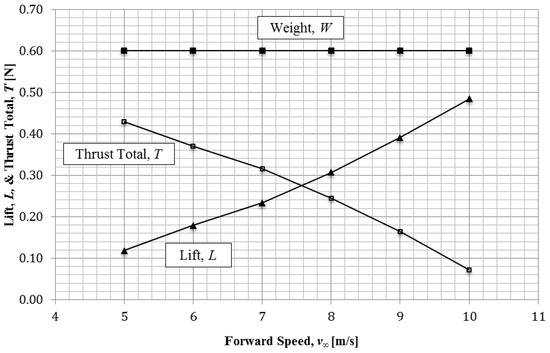
Figure 5.
The replication hypothesis assumes the lift, thrust, and weight curves from a bird to apply also to a protobird. The crossover occurs at a forward speed v∞ of ≈ 7.5 m/s experienced by both flyers.
The database in Table 1 can now be expanded to include and the relevant morphological and kinematic data, resulting in Table 2.
Table 2.
Physically relevant parameters along the take-off run for the bird and an analogous protobird.
The lift activity angle θ, column 3, is calculated using Equation (20) and plotted as a function of the forward speed, v∞, in Figure 6.
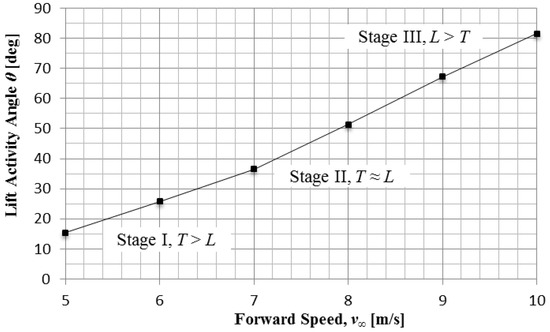
Figure 6.
The lift activity angle θ at various forward speeds.
The flapping velocity, vf, column 5, is found squared in the second term contained in brackets in Equation (11); the wing velocity, vw, column 6, is defined by Equation (11); the Strouhal number, St, equals (2·f·A/v∞); and the kinetic pressure, Q∞, is calculated using Equation (14).
(iii) Calculation of the normalized lift and normalized thrust. The available normalized lift ηL avail, in Table 3 is calculated by normalizing the lift L in Table 1 (that is, solving for ηL in Equation (15)). The required normalized lift ηL req is calculated using the same equation, but normalizing the protobird’s weight, W, of 0.6 N, instead of its lift L. The normalized thrust ηT is obtained by solving for it in Equation (16).
Table 3.
Normalized thrust and available and required normalized lift along the take-off run.
The normalized thrust ηT, the available normalized lift ηL avail, and the required normalized lift ηL req, are plotted in Figure 7:
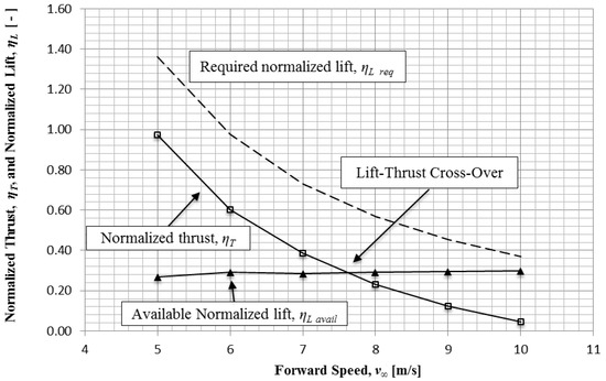
Figure 7.
The normalized thrust, the available, and the required normalized lift for 5 m/s v∞ 10 m/s.
The dashed curve in Figure 7 represents the required normalized lift, ηL req, necessary to achieve flight, which is higher than ηL avail, throughout the velocity interval of 5 m/s v∞ 10 m/s. Hence, the bird and the analogous protobird are not capable of lift-off in this range of forward speeds.
According to the replication hypothesis, the normalized lift, ηL, and normalized thrust, ηT, at a forward speed, v∞, of, say, 7 m/s, Figure 7, correspond to an instant that finds the bird accelerating towards take-off, and also to a protobird that runs at the same maximum speed, v∞, that is, in horizontal equilibrium. Note that whereas the bird accelerates through the 7 m/s mark (T > D), the protobird is found running at this speed of 7 m/s while in horizontal equilibrium, (T = D), while exerting maximum flapping power. Based on these different conditions encountered by the bird and protobird, a more appropriate graph is discussed in Section 6.
4.2. The Cost of the Kinetic Energy of a Wing’s Cyclic Pitch
The normalized lift ηL and the thrust ηT are formally calculated by normalizing L and T by the total specific kinetic energy ek available at the flapping wing, as stated by the term Σeki, in Equation (4). From a practical perspective, only two sources of kinetic energy have been considered, namely, the kinetic energy due to translation, ek trans, and due to flapping, ek flap. A neglected source is the wing’s kinetic energy, ek pitch, due to its cyclic pitch around its spanwise axis as it pronates and supinates at each flapping cycle. The following equation for the normalized lift, ηL, follows more closely its definition as it uses of the total kinetic energy available at the flapping wings for normalizing L:
The specific kinetic energy, ek pitch, corresponds to the wing’s cyclic pitch along an angle Φpitch of, say, 20° (0.35 radians), a kinematic mechanism that allows the wing to act as a propeller by the cyclic adjustment of its pitch angle to the incoming flow in order to generate thrust, Taero, and is equal to
According to physics textbooks, the moment of inertia I of a rectangular flat plate representing, say, the left wing with a rectangular planform of root-to-tip span r (= 0.4 m and chord c (= 0.0645 m), is equal to (1/12∙m∙c2) [5]. The angular velocity due to the cyclic pitch, ωpitch, Equation (9), equals (2∙f∙Φpitch). Replacing, we obtain
The specific moment of inertia, I/m, in Equation (27), equals 0.00035 m2 (= 0.06452/12). The angular velocity due to flapping, ωpitch, equals 4.88 1/s (=2 × 7 × 20/57.3). Replacing these two values in Equation (24) results in the specific kinetic energy of the wing due to cyclic pitch, ek pitch of 0.00417 m2/s2, (= ½ × 0.00035 × 4.882), a negligible value when compared to the average kinetic energy ek available at the wing due to translation and rotation of 29.6 m2/s2 (ek = ½ × vw2 = ½ × 7.72), calculated for a wing velocity, vw, of 7.7 m/s.
The combination of the important role by the wing’s cyclic pitch in the generation of thrust and the accompanying low cost in kinetic energy may have contributed towards thrust being the primordial aerodynamic force along the evolution towards sustained flight.
5. A Second Hypothesis: Equilibrium during Lift-Off
Whereas the replication hypothesis uses aerodynamic data along the take-off of a bird and applies it to a protobird along its evolution (L < W), a second hypothesis states that the horizontal and vertical forces acting on a protobird as it reaches level lift-off (L = W, no ascending flight follows) while exerting maximum power during flapping are in equilibrium. This condition, T = D, is expressed by equating Equations (16) and (17):
Simplifying, we obtain
This equation is not dependent on the dynamic pressure q∞ (= ½·ρ·v∞2).
When level lift-off is achieved by the protobird during maximum power exerted for flapping, then L = W, and so
At this condition, a casual observer witnessing the lift-off of a protobird would not distinguish between its apparent “running” and its actual flying at ground level, as both actions share outwardly similar kinematics but different dynamics. This condition is mirrored by a non-running, non-flapping, flying paraglider, Figure 8, as in both cases, they share the generation of lift equal to their weight, and simulate the running action without generating thrust with their soles.

Figure 8.
A (non-flapping) paraglider mimics the running action while a protobird actually flies at level lift-off. A casual observer would be challenged to distinguish between the running and the flying [10].
With Equations (29) and (30) we have arrived at a system of simultaneous equations describing the dynamics of a protobird at the instant of level lift-off:
A cursory examination of these equations yields two observations:
(i) The overarching aerodynamic ingredient found in both equations is the product of the parenthesis (1 + ⅓∙St2) and the wing planform area, Sp. The result of this product is referred to as the expanded wing planform area, Sp’:
Conceptually, the expanded wing planform Sp’ is a fixed wing planform area with the same capability for generating lift and thrust as the flapping wings. As the Strouhal number, St, and/or the wing planform area, Sp, increases, so does the expanded wing planform area. Equations (31) and (32) are rewritten as
(ii) The second equation, Equation (35), is found “dampened” by the presence of the dynamic pressure, q∞, typically a small value during stages I and II. As this is a lift-related equation, the generation of lift L by flapping wings in their early evolutionary stages may have been adversely affected by its presence.
6. Polar Diagrams
Figure 7 in Section 4(iii) shows the graphs of the normalized lift, ηL, and normalized thrust, ηL, as a function of the forward speed, v∞, of an accelerating bird, and an analogous protobird in equilibrium, a simplified correspondence, as the thrust (and accompanying lift) by an accelerating bird must be somewhat larger than the thrust (and lift) by an analogous protobird in equilibrium, both moving forward at the same speed, v∞. This issue is solved by replacing the forward velocity v∞ by lift activity angle, θ, as the common independent parameter for the bird and analogous protobird.
A polar diagram documents the history of the progression of the resultant vector and the lift activity angle, θ, of a bird along its take-off run, and of an analogous protobird along its evolution towards sustained flight, according to the replication hypothesis. The horizontal axis of the polar diagram represents the normalized thrust, ηT, and the vertical axis of the normalized lift ηL. Any point on the curve can expressed by Euler’s formula [11]:
The resultant vector R is distributed inside the parentheses on the right-hand side of the equation, resulting in the addition of the thrust T and the lift L, both the horizontal and vertical components of the resultant:
Replacing T and L by Equations (16) and (15), and taking out of the parentheses the common factors, we get
Dividing both sides by Q∞∙Sp, we arrive at
The left-hand expression corresponds to the polar notation and the right-hand expression to the Cartesian notation (i.e., “x” and “y” coordinates).
The Instantaneous Polar: Characterizing the aerodynamic condition at an “instant” along a bird’s take-off run or along the protobird’s evolution towards sustained flight can be done by an instantaneous polar, a snapshot that documents the normalized resultant force R, the lift activity angle, θ, the normalized thrust, ηR, and the normalized lift, ηR.
Point A in Figure 9 documents the normalized thrust ηT A and normalized lift ηL A, the resultant ηR A and the lift activity angle θA = 60° (=π/3) of a bird and a protobird. Point B describes the same flyers’ hovering flight at ground level or vertical ascending flight, as there is an absence of thrust, ηT B = 0, and the normalized resultant ηRB equals the normalized lift, ηL B, and the lift activity angle, θB, is 90° (= π/2).
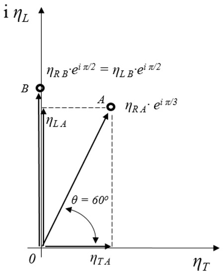
Figure 9.
Two instantaneous conditions. Point B corresponds to hovering or vertically ascending flight.
With the information available, it cannot be said if lift L at point B is larger, equal, or smaller than the weight W, hence, the bird may be standing and flapping, hovering at ground level or in a vertical climb.
This situation is visited below.
The History Polar: The history polar is a succession of instantaneous polars plotted for an increasing value of the lift activity angle θ. A hypothetical history polar, Figure 10, depicted by a dashed line and divided in the three stages, I, II, and III (Section 3), is read from stand-still of the protobird (point 0 in Fig. 10), millions of years ago, and counter-clockwise along the curve, evolving towards its intersection with the vertical axis, at which point, the bird generates only lift, implying flapping at stand-still, hovering at ground level, or in a vertical climb.
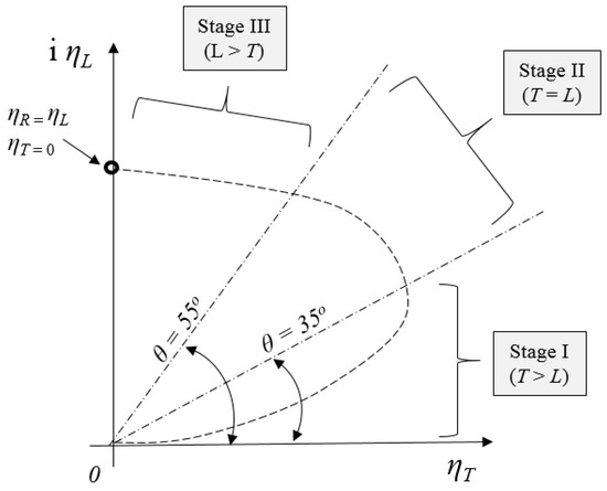
Figure 10.
A hypothetical polar that describes the take-off by an extant bird and the evolution of a protobird towards sustained flight.
To define this undefined flight condition, we refer to point 2, Figure 11, where the required normalized lift of the bird, ηL req, from Equation (18) and repeated below, is added to the history polar, coinciding with, say, point 2:
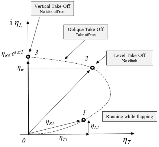
Figure 11.
A hypothetical history polar showing the different performance capabilities of a bird and a protobird.
The presence of this horizontal marker helps clarify the fact that, at point 2, the protobird reaches the condition ηL = ηreq, at which point it first encounters level lift-off, L = W, while “running” (actually flying) without the capability of ascending flight. Moving counterclockwise from point 2, the protobird, now referred to as a bird, generates L > W and is capable of ascending flight (i.e., oblique lift-off), reaching altitudes, at first, measured in centimeters.
Discussed next are (i) the possible presence of an initial polar slope and (ii) the thrust inflection point at the polar’s “3 o’clock position”, point 7, Figure 12.
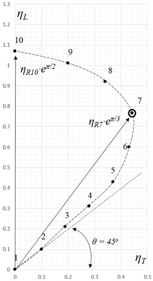
Figure 12.
A history polar presenting a hypothetical linear initial behavior and a thrust inflection point.
The hypothetical history polar of a protobird, Figure 12, shows the first four points, 1 to 4, placed within a small range of lift activity angles, 45° < θ < 48°, which may imply its flapping wings may have had very low or no camber (i.e., acting as flat plates), and have been equally effective generating thrust in their upstroke and downstroke, and, as a result, also generating as much thrust as lift (ηL ≈ ηT) along stage I. Under this assumption, there is no lift-to-thrust crossover to be expected. Admittedly, detecting the presence of this feature may be difficult to capture by documenting the aerodynamic forces along the take-off run of an extant (cambered winged) bird. This topic may be addressed instead by combining the analysis of the generation of lift and thrust by the numerical modeling of low and uncambered wing airfoils in ground effect using computational fluid dynamics, and any fossil evidence for the presence of low or uncambered wings (a significant challenging task).
The thrust inflection point, represented by point 7, Figure 12, corresponds to the same point 7 in Figure 13, a Cartesian version of Figure 12, where the point number (1 to 10) is inscribed along the “x” axis, and the normalized lift, ηL, and normalized thrust, ηT, are found along the “y” axis. The thrust inflection point, point 7, is thus the point of maximum thrust generated along evolution of the protobird (in the case of a polar that intersects the “y” axis).
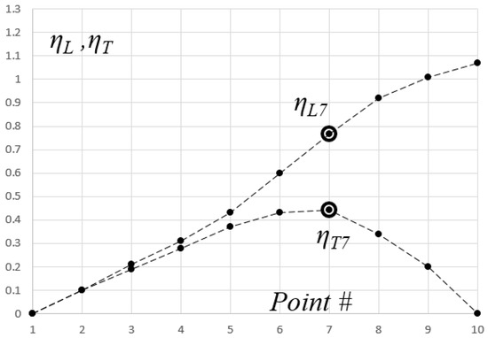
Figure 13.
Hypothetical lift-thrust of flapping wings divergence along their evolution towards sustained flight.
For a hypothetical bird and an analogous protobird with no capability of a vertical lift-off, their history polar may look like the history polar shown in Figure 14, where the bird takes off and climbs at an estimated normalized lift ηL > 0.55, point 6, and the analogous protobird reaches a maximum translational speed, v∞ max, along its evolution towards sustained flight at, say, point 4. This particular history polar does not present a thrust inflection point.
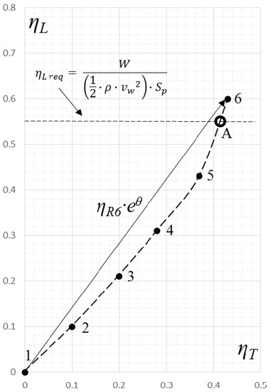
Figure 14.
A hypothetical history polar showing the transition of a protobird into a bird at point A.
For a history polar to present a thrust inflection point, the bird may have to undergo substantial a decrease in weight, W, and/or wing loading W/Sp, and/or increase in wing velocity vw (as discussed in Section 7.3). Although these parameters have been assumed constant throughout the history polar, the equations presented in this paper allow for their variations during the construction of the history polar.
7. Case Studies Involving Level Lift-Off of a Protobird
This section presents three studies related to the level lift-off of a protobird using the same parameters as in Section 4. The wings operate at a normalized lift, ηL of ≈ 0.45.
7.1. Vertical Forces during Level Lift-Off
We calculate the wing velocity vw min required for the generation of a lift L equal to its weight of 0.6 N, using the second of the two simultaneous equations, Equation (18):
This results in a wing velocity, vw min, of 9.158 m/s that will generate a lift equal to the weight of the protobird, making possible its level lift-off, without the ability for ascending flight.
7.2. Horizontal Forces in Equilibrium at Near Take-Off
At level lift-off, a flapping protobird translates at its maximum forward velocity v∞ min while exerting maximum flapping power, and attains a wing velocity vw min fly in order to generate L = W while flying at ground level. At this condition, its flapping wings generate a thrust T that equals its drag D, Equation (31):
This equation calculates the normalized thrust ηT at which the wing is operating during the generation of thrust. The two unknowns are the frontal area, Sf, and the normalized drag, ηD. The frontal area Sf is calculated using the allometric equation suggested by Pennycuick et al. for passerine species [12]. For a mass m of 0.0612 kg, we obtain
This value assumes a streamlined body aligned to the flow and hindlimbs retracted. In contrast, the translating protobird may have a more erect body attitude and have its hindlimbs exposed (causing high drag as they involve small Reynolds numbers). The frontal area, Sf, is thus doubled, estimated to be ≈ 0.005 m2. The normalized drag ηD in Equation (17) equals the drag coefficient CD, using frontal area Sf as Sref, and is calculated using the following regression equation [13]:
ηD = CD = 0.82 − (7.5 × 10⁻⁶)∙Re = 0.82 − (7.5 × 10−6) × 40,000 = 0.51
Using the same rationale, the protobird with a more erected body and exposed hind limbs is estimated to have a higher normalized drag ηD, and it is assumed to be ≈ 0.65. The right-hand side of Equation (44) (= ηD∙Sf) equals 0.00325. Solving for the normalized thrust results in ηT ≈ 0.121.
7.3. Effect of Flapping Frequency fmin on the Forward Speed v∞ min Required for Lift-Off
The minimum wing velocity, vw min, required for generating a lift equal to the weight of the protobird for initiating level lift-off, Equation (10), is rewritten below:
Level lift-off is reached when a combination of minimum forward speed, v∞ min, flapping frequency fmin and minimum amplitude Φmin for a given wing length r results in the minimum wing velocity vw min required for generating a lift equal to its weight.
This section calculates the required increase of the minimum wing flapping frequency, fmin, as a hypothetical protobird evolves from a level lift-off (L = W) at a translation speed, v∞ min, and flapping at fmin = 7 Hz (point B in Figure 15) towards a “hummingbird-type” flyer capable of hovering at L = W (no lifting off vertically), point C in Figure 15, at v∞ min fly = 0. For simplicity, we assume a constant wing velocity, vw min, of 9.158 m/s, as calculated in Section 7.1. From Equation (46), vw min is:
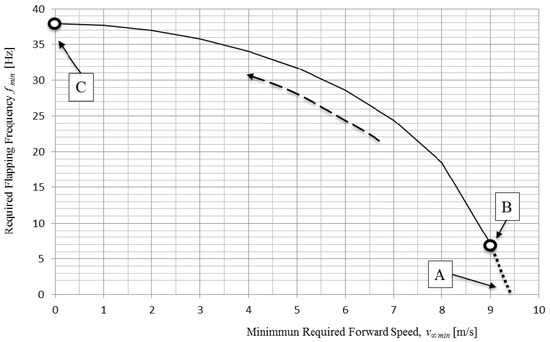
Figure 15.
The effect of forward velocity v∞ on flapping frequency f for a constant wing velocity vw as the wing generates a lift L equal to the weight W of the protobird.
The subscript “min” indicates that the parameters have the minimum value that is required for generating L = W. From Section 7.1 we have found that the minimum wing velocity, vw min, for reaching L = W, is 9.158 m/s. From the above equation, we solve for fmin:
Keeping the wing velocity vw min constant (not realistic in evolutionary terms), the translation velocity, v∞ min, is varied from 9 m/s to zero, resulting in an increase in the flapping frequency fmin, as shown by the dashed arrow in Figure 15.
The initial point A in Figure 15 shows the protobird taking off with its fixed wings, in “airplane mode”, a condition that does not concern us. Point B is the initial condition of this case study that finds the early protobird flapping its wings at a frequency fmin of 7 Hz while translating at a velocity, v∞ min, of 9 m/s (Table 2). Evolving towards point C, v∞ min → 0, and the required flapping frequency, fmin, increases to 37.87 Hz. At this time, L = W and the (now) bird is capable of a hummingbird-like hover at ground level. If fmin > 37.87 Hz, the bird is capable of vertical ascending flight. As a reference, current hummingbirds hover by flapping their wings at a frequency between 12 and 80 Hz [14].
The evolution towards vertical lift-off is a process lasting vast periods of time and, in all likelihood, is accompanied by one or more (or all) of the following changes: a substantial reduction in weight, a reduction in wing loading, an increase in the length of the wing (towards a higher aspect ratio, 2∙r/), and a substantial increase in flapping amplitude (to possibly double the amplitude of 60°, as considered in this paper) and, most importantly, the power available for allowing for a high flapping frequency as the results in this section may indicate.
If the fossil record shows evidence that one or more of these changes have occurred, a detailed history polar of a protobird that reflects these changes must rely on the appropriate (experimental) lift and thrust database of the corresponding birds reflecting these changes.
8. Conclusions
The common theme throughout the paper is that flapping wings contribute to the survival skill of a predator or a prey, namely, forward speed. In other words, the “objective” during evolution (there is no objective per se during evolution) may be maximizing forward speed, not lift, as thrust is the common thread along the evolution towards sustained flight. Ironically, the generation of thrust disappears when the bird reaches the epitome of flight: vertical lift-off and hover. Relatively small flapping wings may contribute to thrust to run faster (i.e., chicken). Larger wings may contribute to lift-off after a lengthy take-off run, which increases the forward velocity. Smaller wings flapping at high frequency may end up enabling the bird to lift off vertically, an operating condition that has no need for the generation of thrust. A bird that possesses the ability to lift off vertically and hover can relinquish the need for thrust.
All these aerodynamic conditions can be evaluated experimentally and numerically by applying the replication hypothesis and the simultaneous set of equilibrium equations at the moment of level lift-off.
Reaching a consensus on an idea, which is usually expected to occur over time, seems particularly challenging when delving on the subject of the origin of sustained flight. A reason for this may be the lack of a numerical approach and, as a result, jumping, leaping, climbing, and falling have appeared to be credible steps by flapping wings in their early evolution towards sustained flight. Little can be done to counter these arguments without a physics (that is, numerical) approach to the subject.
The author applauds the experimental approach (i.e., WAIR, [15]) used by Professor Dial, and coauthors that show the importance of flapping in the generation of thrust by an evolving protobird. I may dare argue that the WAIR experiments are close in spirit to the first stage of the replication hypothesis, as these help generate the experimental lift and thrust database that help construct the analogous (early) protobird’s history polar.
Any approach towards promoting a hypothesis that explains the origin of sustained flight is, by its nature, conjectural and, as such, unlikely ever to be tested. On the other side, Sir Humphrey Davy has stated that the only use of a hypothesis (or two) is to lead us to experiments to guide us to facts. With these thoughts in mind, this paper presents two falsifiable hypotheses, the replication hypothesis and the equilibrium hypothesis. The first hypothesis applies a (preferably experimental) lift and thrust data obtained from a bird along its take-off run to an analogous protobird, as deconstructed from the paleontological fossil evidence. The aerodynamic basis of the evolutionary process (basically the ratio of lift to thrust) towards sustained flight of flapping wings, lasting millions of years, is scaled down to a matter of seconds. As the maximum forward velocity of the “running” protobird gradually increases and finally reaches level lift-off, the second hypothesis suggests it being subjected to vertical and horizontal forces in equilibrium.
This multidisciplinary approach, with contributions from physics (Newton’s 1st and 2nd laws applied throughout this paper), aerodynamics (Prandtl’s q∞), paleontology (Darwin) and mathematics (Euler’s equation), allows for the numerical and graphical fine-tuning of the protobird’s model along its evolution to account for possible variations in weight, morphology, kinematics, and dynamics over time, according to the latest findings in the fossil record.
Acknowledgments
The author gratefully acknowledges the contributions by Christy Anderson and Steven Kast for helpful comments, Philip Mugridge for photograph, and Allison Elain Johnson for drawing in graphic abstract, and an anonymous reviewer for discussions.
Conflicts of Interest
The author declares no conflict of interest.
Glossary
| A | arc subtended by the wing tip |
| CD | drag coefficient |
| CL | lift coefficient |
| CT | thrust coefficient |
| average wing chord | |
| D | drag |
| Ek | kinetic energy |
| ek | kinetic energy per unit mass, Ek/m |
| F | aerodynamic force, lift, thrust, drag |
| f | flapping frequency |
| fst | stroke frequency |
| I | moment of inertia of wing |
| L | lift |
| m | mass of flyer, mass of fluid parcel |
| Q∞ | kinetic pressure |
| q∞ | Prandtl’s dynamic pressure |
| R | resultant of the lift and thrust vectors |
| Re | Reynolds number |
| Sf | frontal (reference) area |
| Sp | wing planform (reference) area |
| Sp’ | expanded reference area, (1 + ⅓∙St2)∙Sp |
| St | Strouhal number |
| T | thrust |
| vf | flapping velocity |
| vtt | tangential wing tip velocity |
| vw | wing velocity |
| v∞ | translating (forward) velocity |
| W | weight of flyer |
| w | work per unit mass of flyer |
| ρ | density of air |
| ηD | normalized drag |
| ηL | normalized lift |
| ηT | normalized thrust |
| Φ | flapping amplitude |
| ω | angular velocity of flapping wings |
| μs | static friction coefficient |
References
- Burgers, P.; Chiappe, L.M. The wing of Archaeopteryx as a primary thrust generator. Nature 1999, 399, 60–62. [Google Scholar] [CrossRef]
- Burgers, P. Comparison of the average lift coefficient and normalized lift for evaluating hovering and forward flapping flight. Aerospace 2016, 3, 24. [Google Scholar] [CrossRef]
- Burgers, P. Dimensionally and physically proper lift, drag and thrust-related numbers as figures of merit: Normalized lift, drag and thrust ηL, ηD, and ηT. J. Aerosp. Eng. 2016, 30, 04016091. [Google Scholar] [CrossRef]
- Resnick, R.; Halliday, D.; Krane, K.S. Physics, 4th ed.; Wiley: Hoboken, NJ, USA, 1992; Volume 1. [Google Scholar]
- Prandtl, L. Applications of Modern Hydrodynamics to Aeronautics; NACA-TR-116; National Advisory Committee for Aeronautics: Washington, DC, USA, 1921.
- Lentink, D.; Dickinson, M.H. Biofluiddynamic scaling of flapping, spinning and translating fins and wings. J. Exp. Biol. 2009, 212, 2695. [Google Scholar] [CrossRef] [PubMed]
- Puffin Photograph by Tom Grey. Available online: http://www.pbase.com/tgrey (accessed on 6 June 2018).
- Hummingbird Photograph. Available online: https://commons.wikimedia.org/w/index.php?curid=12374160 (accessed on 28 March 2018).
- Malik, M.A.; Ahmad, F. Effect of different design parameters on lift, thrust and drag of an ornithopter. In Proceedings of the World Congress on Engineering, London, UK, 30 June–2 July 2010. [Google Scholar]
- Zsolt, H. Available online: http://www.sikloernyostanfolyam.hu/hu/paraglidinghungary (accessed on 15 April 2018).
- Needham, T. Visual Complex Analysis; Oxford University Press: Oxford, UK, 1997. [Google Scholar]
- Nudds, R.L.; Rayner, J.M.V. Scaling of body frontal area and body width in birds. J. Morphol. 2006, 267, 341–346. [Google Scholar] [CrossRef] [PubMed]
- Hedenstrom, A.; Liechti, F. Field estimates of body drag coefficient on the basis of dives in passerine birds. J. Exp. Biol. 2001, 204, 1167–1175. [Google Scholar] [PubMed]
- Puttick, M.N.; Thomas, G.H.; Benton, M.J. High rates of evolution preceded the origin of birds. Evolution 2014, 68, 1497–1510. [Google Scholar] [CrossRef] [PubMed]
- Heers, A.M.; Tobalske, B.W.; Dial, K.P. Ontogeny of lift and drag production in ground birds. J. Exp. Biol. 2011, 214, 717–725. [Google Scholar] [CrossRef] [PubMed]
© 2019 by the author. Licensee MDPI, Basel, Switzerland. This article is an open access article distributed under the terms and conditions of the Creative Commons Attribution (CC BY) license (http://creativecommons.org/licenses/by/4.0/).