Challenges of Fully-Coupled High-Fidelity Ditching Simulations

Abstract

An important element of the process of aircraft certification is the demonstration of the crashworthiness of the structure in the event of an emergency landing on water, also referred to as ditching. Novel numerical simulation methods, that incorporate the interaction between fluid and structure, open up a promising way to model ditching in full scale. This study focuses on two main issues of high-fidelity ditching simulations: the development of a suitable fluid-structure coupling framework and the generation of the structural model of the aircraft. The first issue is addressed by implementing a partitioned coupling approach, which combines a finite volume hydrodynamic fluid solver as well as a finite element structural solver. The developed framework is validated by means of two ditching-like experiments, which consider the drop test of a rigid cylinder and a deformable cylindrical shell. The results of the validation studies indicate that an alternative to the standard Dirichlet-Neumann partitioning approach is needed if a strong added-mass effect is present. For the full-scale simulation of aircraft ditching, structural models become more complex and have to account for damage. Due to its high localization, the damage creates large differences in model scale and usually entails severe non-linearities in the model. To address the issue of increasing computational effort for such models, the process of developing a multi-scale model for the simulation of the failure of fuselage frames is presented.

1. Introduction

Commercial transport aircraft often fly above open waters and, thus, have to prove the safe landing on water. This process is also referred to as ditching and is part of the certification specifications by the European Aviation Safety Agency (EASA) and the Federal Aviation Administration (FAA) (see [1,2]). Those regulations aim for minimizing the risk of injury for the occupants of the aircraft during the impact phase as well as allowing a safe evacuation in the subsequent floatation phase. This requires an accurate prediction of the structural behaviour of the aircraft during the impact phase as well the damage and its influence on the floatation capabilities.

A common practice to certify aircraft for ditching is to compare the new structural design with existing aircraft configurations [3]. As this approach impedes the development of novel, unconventional aircraft configurations, contemporary aircraft design relies on alternative methods to analyse ditching. Experimental investigations of ditching are limited to low horizontal speed (e.g., helicopters [4]) or are conducted on model scale [5,6] where they suffer from scaling effects, particularly with respect to the accurate representation of hydrodynamic effects [7]. Consequently, there is a motivation to employ numerical tools to simulate ditching. Those tools can be broadly classified into high-fidelity and low-fidelity approaches. High-fidelity methods are based upon general computational mechanics and usually employ particles or a mesh to discretize the aircraft structure and the surrounding fluid. Conversely, low-fidelity methods discretize structure and fluid in a simplified manner and are based on analytical or semi-analytical formulations (see e.g., [8,9]). Those tools are often used in the context of a one-way coupling approach, where the hydrodynamic loads are calculated by simplified models and are subsequently applied to a high-resolution finite element (FE) model. In summary, it can be stated that, due to the impracticability of full-scale tests, the limitations of model scale experiments as well as the simplifications in numerical approaches, there is a demand for advanced, high-fidelity simulation methods.

The development of such methods is an active field of current research. Many publications focus on the simulation of ditching events at zero or low horizontal speed (see e.g., [4,10,11]). This condition is normally met during the ditching of helicopters for which results of full-scale experiments are available and are used to validate simulations [4]. Conversely, the ditching of fixed-wing aircraft involves a significant horizontal speed and, therefore, hydrodynamic effects such as cavitation, ventilation and the formation of bow waves and spray jets need to be considered [3,12]. These physical effects present additional numerical challenges compared to helicopter ditching.

Furthermore, the large hydrodynamic loads arising in the impact zone usually rise and fall within milliseconds and therefore require small time step sizes in the fluid simulation [3]. Those loads result in local structural deformation and possibly failure. Moreover, failure occurring in fuselage frames usually occurs locally as well. If modelled using a high-resolution FE discretization, this may lead to large differences in model scale [13].

As the flexibility of the structure has a significant effect on the hydrodynamic loads acting on the structure during the ditching event, fluid-structure interaction (FSI) needs to be considered [14]. Due to the specific requirements of the individual solvers, monolithic coupled solvers are not practical. Instead, a partitioned coupling approach is required.

The process of ditching is accompanied by a strong added-mass effect of the fluid on the structure [15]. This gives rise to numerical instabilities in the coupled solution, particularly if fluid and structural densities are comparable, the structure is slender and incompressible flow is assumed [16,17,18]. Iterative (implicit) coupling methods have been widely adopted to simulate strongly coupled problems with a pronounced added-mass effect (see e.g., [19,20]). However, those methods may also suffer from stability issues and increased computational effort [18]. It is therefore crucial to employ an efficient partitioned procedure in order to make highly resolved ditching simulations feasible.

Current high-fidelity methods usually employ the FE method to simulate the structural response of the aircraft. Conversely, the fluid domain typically is discretized by using either a mesh-free approach (see e.g., [21]) or a hybrid approach. The latter combines classical Lagrangian FE methods with smoothed-particle hydrodynamics (SPH) to alleviate the problem of growing computational effort with larger fluid domains (see e.g., [3,6,22]). The advantage of such particle methods is that they eliminate the issue of mesh deformation in the fluid domain. However, cavitation is only accounted for in a simplified manner by cutting off the pressure as soon as it falls below a defined minimum value [3,23]. Hence, both phase changes and the presence of vapour are not considered, although those effects may considerably influence the hydrodynamic loads of the fluid on the structure [8,24]. This can be remedied by using the finite volume (FV) method for which cavitation models are already available and tested (see e.g., interPhaseChangeFoam solver in OpenFOAM 5).

The focus of this study is twofold: a suitable fluid-structure coupling framework is presented and validated using the two-dimensional drop test of a rigid cylinder and a deformable cylindrical shell. Furthermore, the process of developing a multiscale model, which simulates the failure of fuselage frames, is illustrated. The paper is structured accordingly: the next section introduces the numerical framework as well as an implicit fixed-point coupling scheme. In Section 3.1, this scheme is employed to simulate the validation problems mentioned above. The elastic validation problem will additionally be simulated using a simple staggered coupling scheme. Section 3.2 deals with the development of a multiscale structural model of the aircraft fuselage. The particular challenge is to accurately model structural failure while limiting the computational effort to a manageable amount. A summary along with conclusions are given in Section 4.

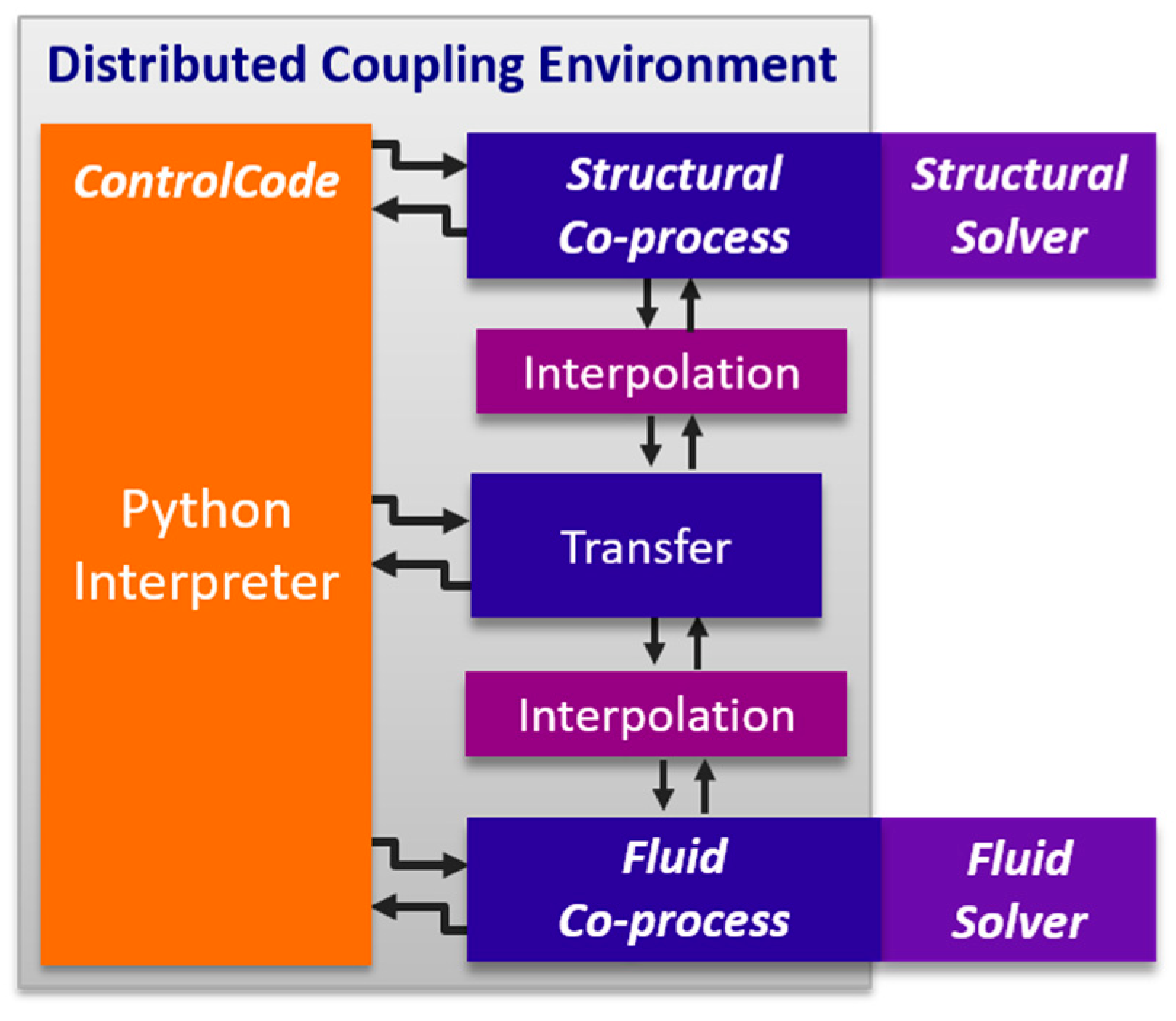
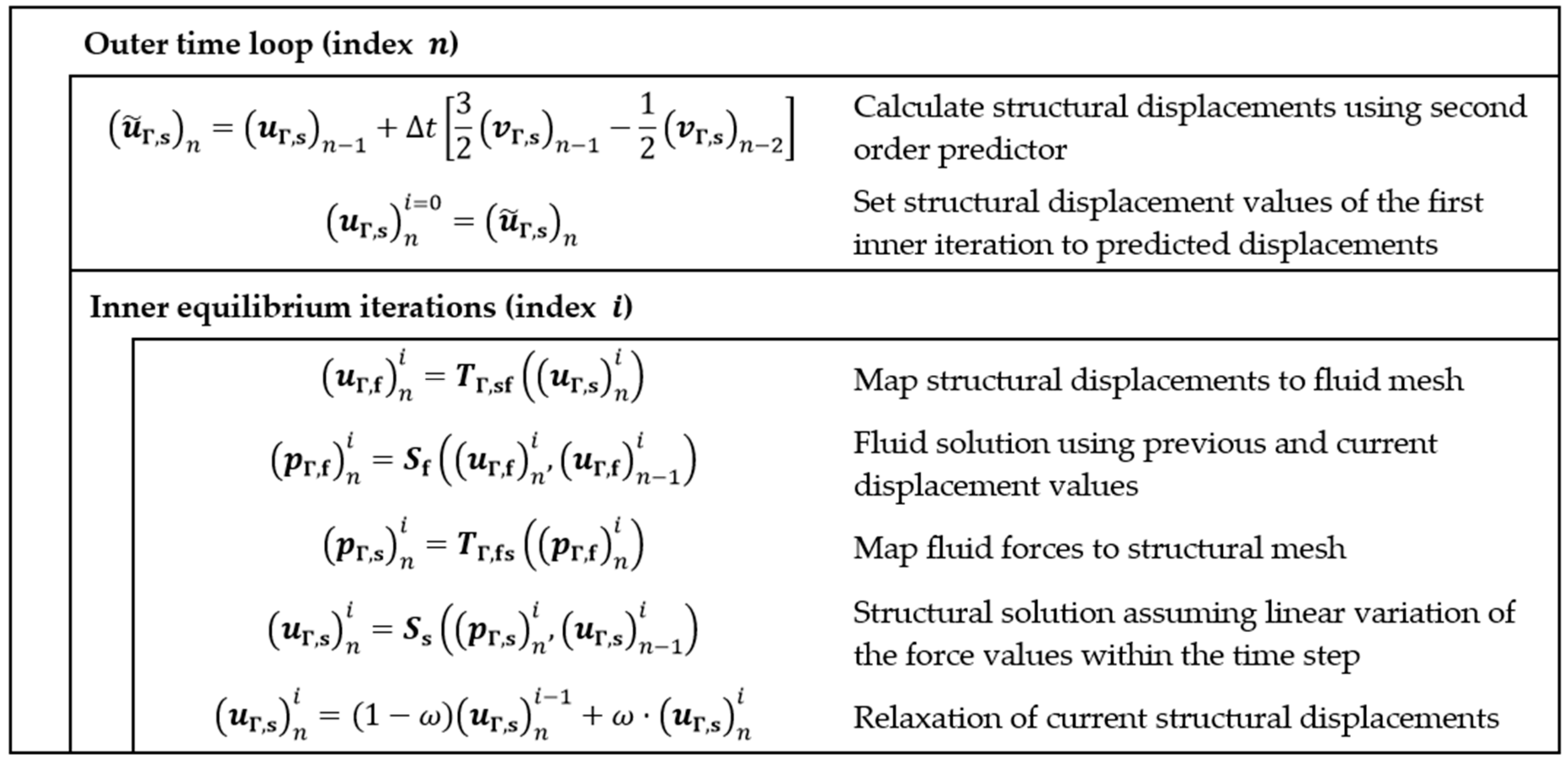
2. Numerical Simulation Framework

This study employs the coupling environment ifls, which has already been used to model various multi-physics problems (see e.g., [25,26,27]). Ifls follows a modular approach that allows to couple two or more black-box solvers in a partitioned way. The usage of the interpreted, high-level programming language Python facilitates a flexible and easy implementation of the desired coupling scheme. Time-critical operations are performed using compiled code as well as the NumPy library. Figure 1 shows the individual processing units of ifls. Simulation steering and solver communication are performed by the control code and the co-processes, respectively. Each of those units is run in a separate thread.

The control code implements the selected partitioned coupling scheme and sends control commands to the co-processes. Those commands provide direct control over the respective solvers and employ a predefined set of instructions that includes, for example, solving a time step or defining and obtaining boundary conditions. Additional instructions for sending and receiving coupling quantities enable access to the coupling data. NumPy is used to store those data and perform arithmetic operations, thus circumventing the speed limitations of Python. If coupling data is exchanged between different surface meshes, the send and receive instructions implicitly invoke appropriate interpolation routines, which are implemented in converter objects and employ methods from the visualisation toolkit (VTK) (The visualization toolkit is Open-Source software, which can be downloaded from https://www.vtk.org.) As the interpolation is computationally more expensive, all interpolation filters are implemented in C++. Another advantage of the usage of VTK is that it facilitates the easy visualization of the simulation results.

Each co-process implements the instruction set used by the control code where basic features common to all co-processes, for example, inter-thread communication and quantity array management, are separately implemented in a generic parent class. Communication between a co-process and the corresponding solver can be achieved in different ways. In this case, a socket-based approach is employed, which has superior performance compared to a simple file-based data exchange. Further information on the coupling environment ifls as well as its underlying principles can be found in Reference [28].

For the simulation of the fluid domain, the finite-volume solver interDyMFoam, which is part of the OpenFOAM 5 toolbox, is employed. It solves the incompressible Navier-Stokes equations and is able to model multiphase flow by means of the Volume of Fluid (VOF) method. The fluid equations are solved in the Arbitrary Lagrangian-Eulerian (ALE) form to account for mesh movement in the convective term. The communication between ifls and OpenFOAM is achieved by using a socket-based data exchange as presented in Reference [29]. The structure is simulated with the implicit Abaqus solver assuming linear elastic material behaviour.

The general partitioned FSI problem can be formulated as follows. The computational domain $\mathsf{\Omega }$ is divided into the structural domain ${\mathsf{\Omega }}_S$ and the fluid domain ${\mathsf{\Omega }}_F$ including their respective boundaries $\partial {\mathsf{\Omega }}_S$and $\partial {\mathsf{\Omega }}_F$. Both domains share the common boundary ${\Gamma }_i\stackrel{\mathrm{def}}{=}\partial {\mathsf{\Omega }}_S\cap \partial {\mathsf{\Omega }}_F$, referred to as the FSI interface, on which the coupling values are exchanged. On the fluid side of the interface, the Dirichlet boundary condition

$${\mathit{v}}_{\mathbf{f}}={\mathit{v}}_{\mathbf{s}},\mathrm{on}{\mathsf{\Gamma }}_{\mathrm{i}}$$

(1)

is applied, where ${\mathit{v}}_{\mathbf{f}}$ and ${\mathit{v}}_{\mathbf{s}}$ represent the fluid and structural velocity vector. Equation (1) corresponds to a no-slip velocity boundary condition in the fluid domain.

Conversely, the fluid forces are applied as a Neumann boundary condition to the structural domain:

$${\mathit{\sigma }}_{\mathbf{f}}\mathit{n}={\mathit{\sigma }}_{\mathbf{s}}\mathit{n},\mathrm{on} {\mathsf{\Gamma }}_{\mathrm{i}}.$$

(2)

The quantities ${\mathit{\sigma }}_{\mathbf{f}}$ and ${\mathit{\sigma }}_{\mathbf{s}}$ represent the fluid and structural stress tensor, respectively, whereas $\mathit{n}$ denotes the unit normal vector.

Ditching exhibits typical characteristics of a strongly coupled FSI problem. For that reason, the implicit fixed-point iteration procedure summarized in Figure 2 is employed. The variables ${\mathit{u}}_{\mathbf{\Gamma }}$ and ${\mathit{v}}_{\mathbf{\Gamma }}$ contain the nodal displacements and velocities at the interface ${\mathsf{\Gamma }}_{\mathrm{i}}$, whereas ${\mathit{p}}_{\mathbf{\Gamma }}$ represents the nodal forces. The operator $\mathit{S}$ describes the solution in the corresponding computational domain. The mapping of the coupling values at the FSI interface from fluid to structure and vice versa is expressed by ${\mathit{T}}_{\mathbf{\Gamma },\mathbf{fs}}$ and ${\mathit{T}}_{\mathbf{\Gamma },\mathbf{sf}}$. The subscripts $\mathrm{s}$ and $\mathrm{f}$ denote the structural and fluid domain. The index $n$ represents the current time increment, whereas $i$ stands for the current iteration.

The fixed-point scheme is usually suitable for strongly coupled problems, although it requires several equilibrium iterations per time step. To accelerate the convergence, the Aitken relaxation method is used to calculate the relaxation factor $\omega$ [30]. Convergence is checked at the end of each iteration by the following displacement-based criterion:

$${\mathit{r}}_{\mathbf{\Gamma },\mathbf{s}}=\frac{\parallel {({\mathit{u}}_{\mathbf{\Gamma },\mathbf{s}})}_n^{i-1}-{({\mathit{u}}_{\mathbf{\Gamma },\mathbf{s}})}_n^i{\parallel }_2}{\parallel {({\mathit{u}}_{\mathbf{\Gamma },\mathbf{s}})}_n^i-{({\mathit{u}}_{\mathbf{\Gamma },\mathbf{s}})}_{n-1}{\parallel }_2+C}<{\mathit{r}}_{\mathbf{\Gamma },\mathbf{s},\max }$$

(3)

where the constant value $C$ ensures that the denominator does not become zero.

3. Results and Discussion

3.1. Validation Studies

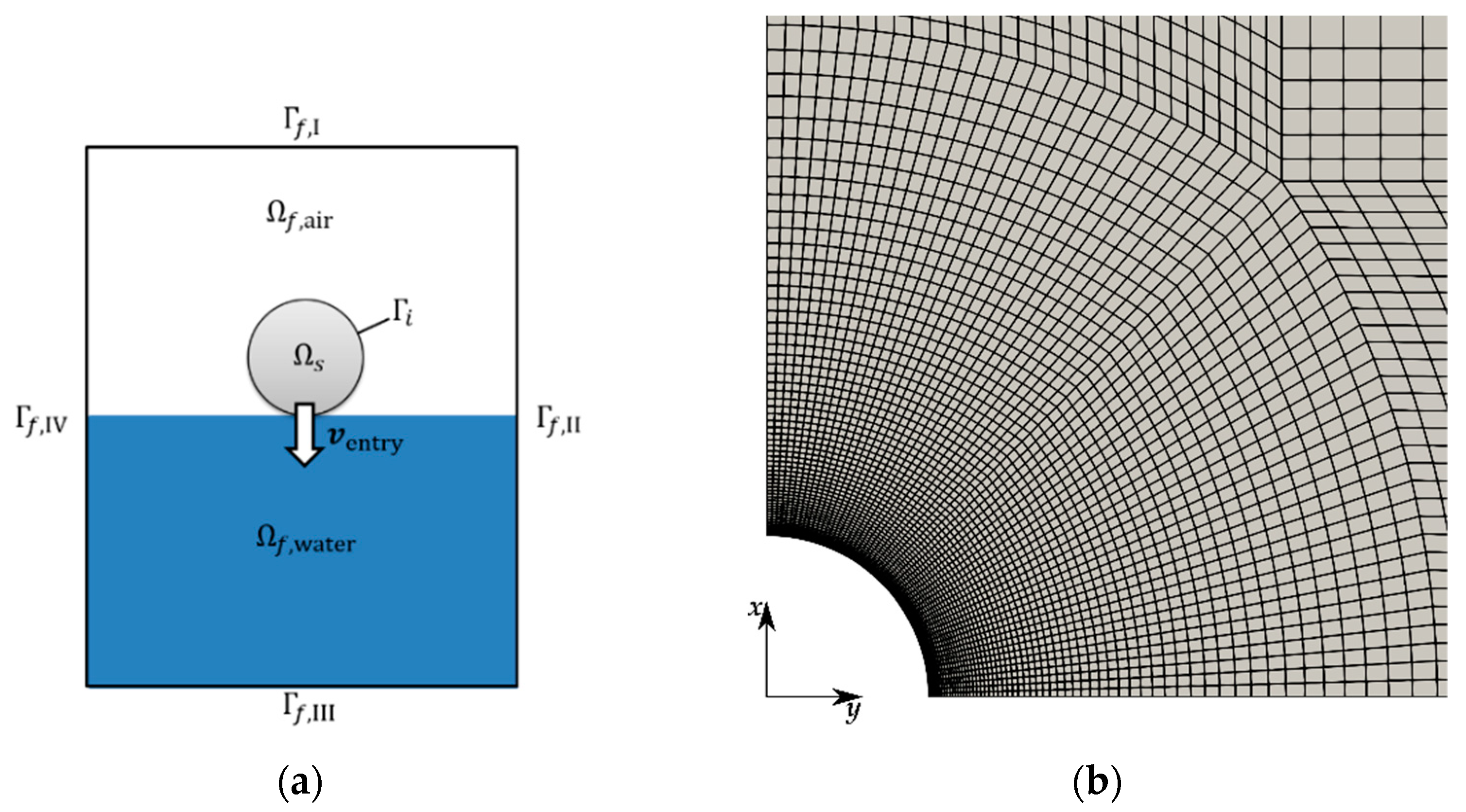
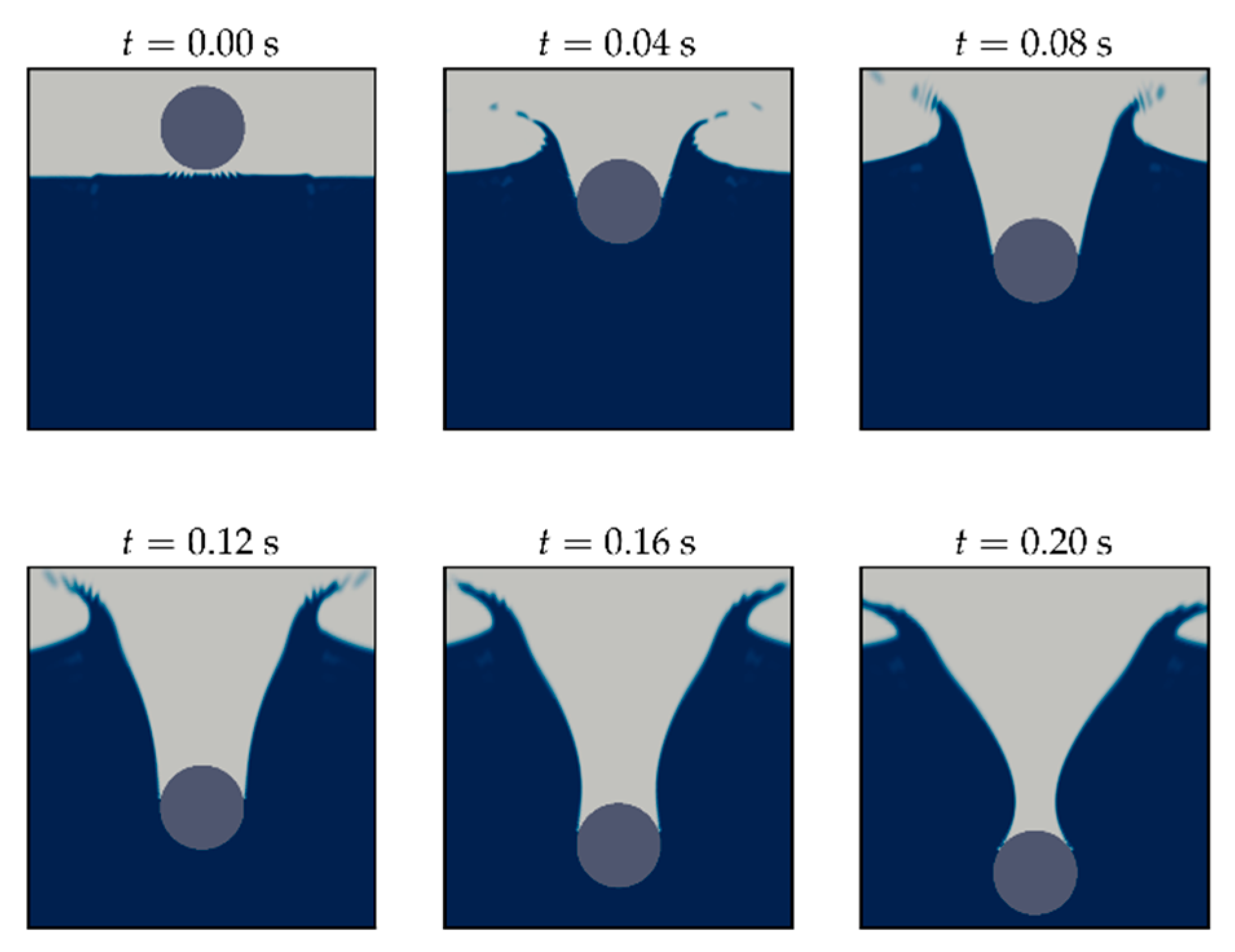
3.1.1. Drop Test of Rigid Cylinder

The model problem of the drop test of a rigid cylinder is based on an experimental study by Greenhow and Lin [31]. The problem set-up as well as the boundaries of the computational domains are shown in Figure 3a. Boundary ${\Gamma }_{f,\mathrm{I}}$ represents the free atmosphere, whereas the boundaries ${\Gamma }_{f,\mathrm{II}–\mathrm{IV}}$ are fixed walls.

Table 1. Boundary conditions in fluid domain.

Boundary	Pressure	Velocity
${\mathsf{\Gamma }}_{f,\mathrm{I}}$	Constant zero pressure	Outflow: zero gradient in normal direction
		Inflow: Robin condition based on flux in the patch-normal direction
${\mathsf{\Gamma }}_{f,\mathrm{II}–\mathrm{IV}}$	Zero gradient in normal direction	Constant zero velocity

summarizes the velocity and pressure boundary conditions which are valid in the fluid domain. Moreover, the interface conditions described in Section 2 are applied on the cylinder surface. The diameter of the cylinder is set to $d=0.11$ m. The mass is chosen in such a way that the cylinder is neutrally-buoyant. The impact velocity amounts to $\left|{\mathit{v}}_{\mathit{entry}}\right|=2.955$ m/s.

The solid is meshed with rigid surface elements where point masses are used to model the mass of the cylinder. The fluid domain is spatially discretized by a two-dimensional block-structured mesh with an O-Grid around the cylinder. A section of the initial fluid mesh mesh02 is shown in Figure 3b. This mesh consists of 22k cells and is constructed from 90 elements along the outer edges ${\Gamma }_{f,\mathrm{I}}$ and ${\Gamma }_{f,\mathrm{III}}$ to 120 elements along ${\Gamma }_{f,\mathrm{II}}$ and ${\Gamma }_{f,\mathrm{IV}}$. The mesh density increases in closer proximity to the cylinder. Additionally, two h-refinement steps are performed. The resulting meshes are labelled mesh03 and mesh04 and contain 89k and 355k cells, respectively. For the simulation of the rigid validation case, the medium fine mesh03 is used.

Fluid and structural simulation are coupled employing the fixed-point iteration scheme described in Section 2. The displacement residual is set to $r_{\mathbf{\Gamma },\mathbf{s},\max }={10}^{-7}$ m, while a constant time step size of $2.5\times {10}^{-5}$ s is chosen. In the structural simulation, the time integration is done by an implicit Newmark-beta method, whereas the fluid solver uses the implicit Euler method. Furthermore, the volume of fluid method in combination with the so-called Multi-Dimensional Limiter for Explicit Solution (MULES) interface compression scheme is employed to model the free water surface. For a detailed description of that scheme, see for example [32].

Figure 4b depicts the depth of penetration over the time and shows good agreement between simulation and experiment. However, the illustration of the different stages of water impact in Figure 5 reveals that the free water surface is not perfectly sharp at the beginning of the simulation. This indicates a strong dependence of the MULES method on the mesh geometry, which was for example also found in Reference [33]. As the simulation results match the experimental results well, it can be assumed that this effect does not have a significant influence on the overall hydrodynamic loads.

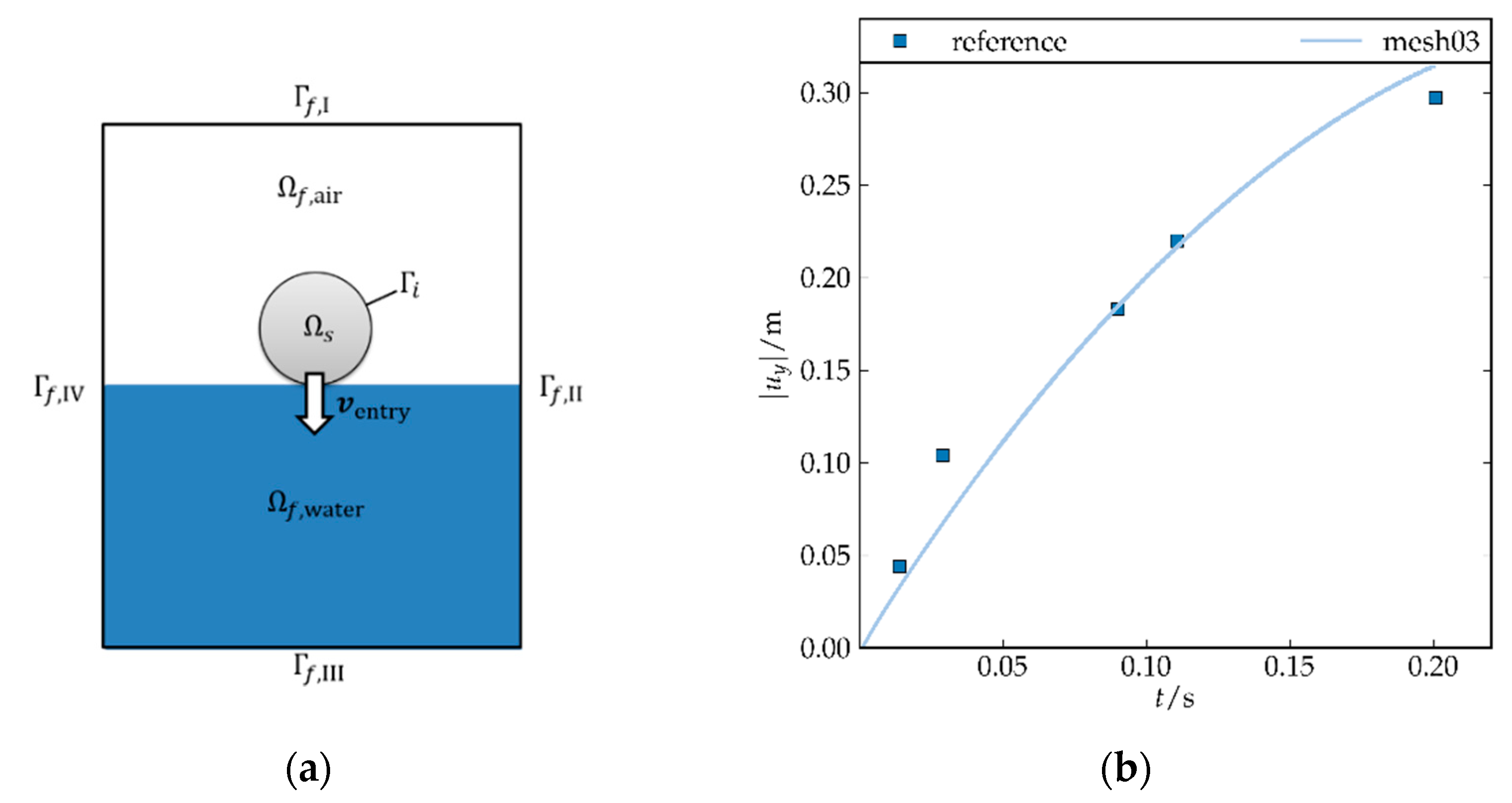
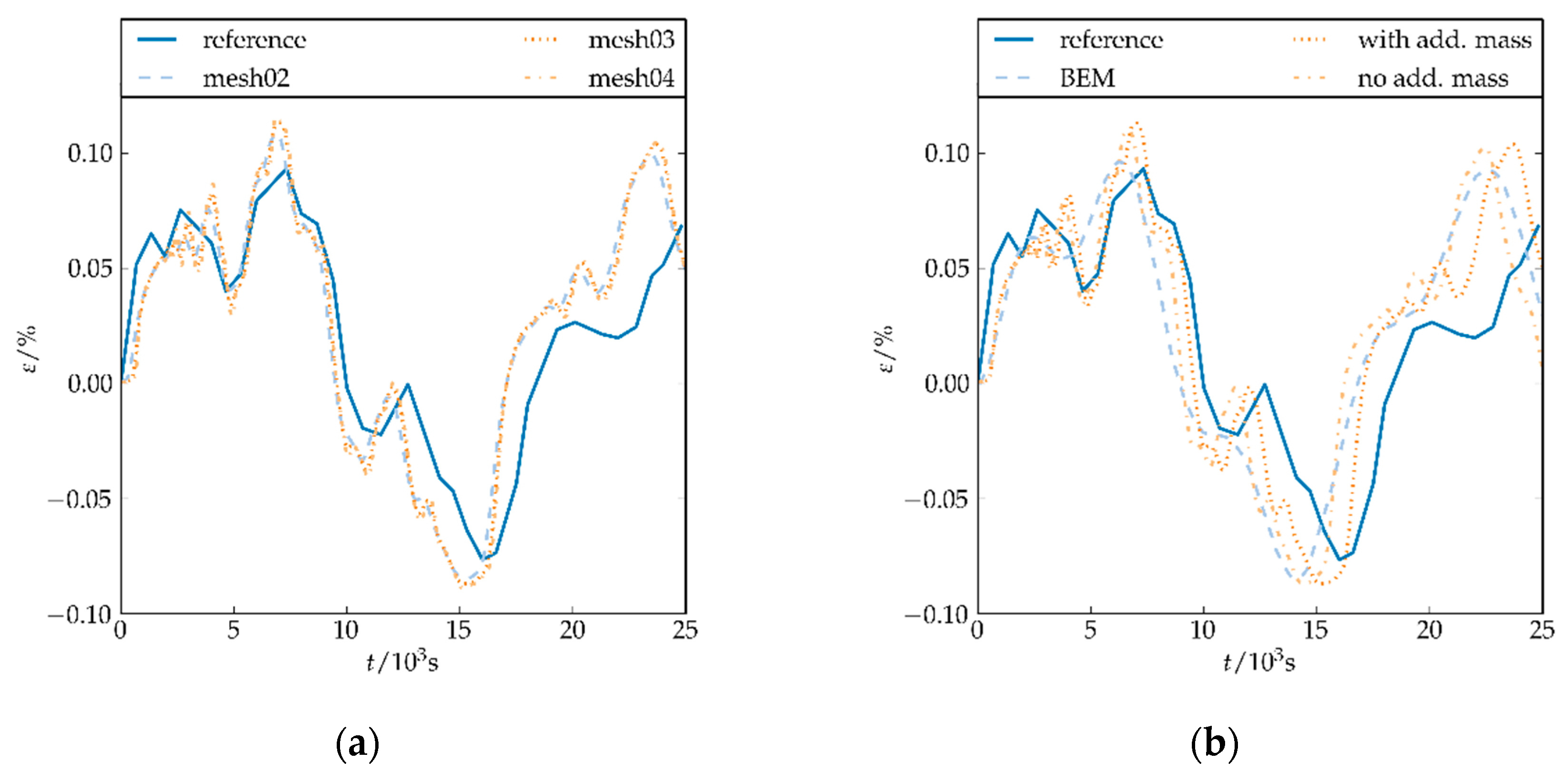
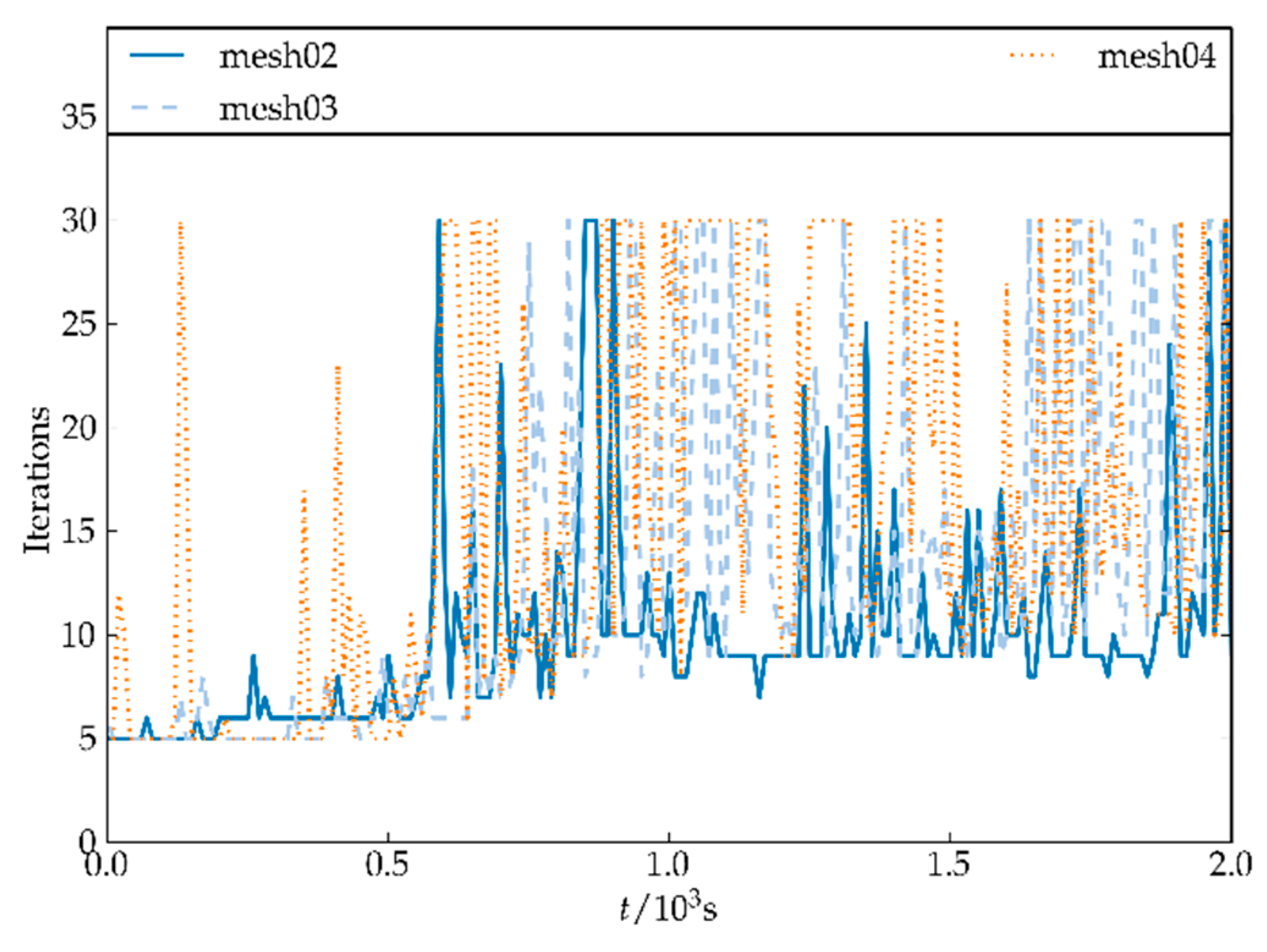
3.1.2. Drop Test of Deformable Cylinder

The elastic validation case is based on [34] by Arai and Miyauchi. In their study, the impact of cylindrical shells on water is both experimentally and numerically investigated. The parameters of the second validation case are summarized in

Table 2. Parameters of elastic validation case.

Parameters	Value
Outer cylinder diameter	$d=0.306 \mathrm{m}$
Shell thickness	$t=3\times {10}^3\mathrm{m}$
Entry velocity	$\left|{\mathit{v}}_{\mathbf{entry}}\right|=3.968 \mathrm{m}/\mathrm{s}$
Shell density	${\rho }_{s,1}=2.70\times {10}^3\mathrm{kg} {\mathrm{m}}^{-3}$
	${\rho }_{s,2}=3.04\times {10}^3\mathrm{kg} {\mathrm{m}}^{-3}$
Young’s modulus	$E_s=7.35\times {10}^{10}\mathrm{Pa}$
Poisson’s ratio	${\nu }_s=0.34$

.

As proposed in Reference [35], the friction of the sliding system in the experiment taken into account by assuming that the water entry velocity is reduced by 10% to the value shown in Table 2. Furthermore, following a simplified approach proposed by Ionina and Korobkin in Reference [36], additional masses due to cables and connectors are considered through an increase of the shell density by 11%, that is assuming those masses are uniformly distributed. In this context, ${\rho }_{s,1}$represents the density without additional mass, whereas ${\rho }_{s,2}$ stands for the cylindrical shell with additional mass.

Despite different dimensions, the discretization of the fluid model is equivalent to the one described in Section 3.1.1, except that all three fluid mesh configurations are investigated in the deformable validation case. The time step is set to a constant value of $1\times {10}^{-5}$ s. The time integrators used in the fluid and structural subsystem are the same as for the rigid validation case. The structural mesh shown in profile in Figure 6 consists of elastic shell elements with linear form functions.

It represents the coarsest resolution and is used in combination with mesh02. For the finer configurations mesh03 and mesh04, h-refinement steps are similarly applied to the structural mesh. Again, the implicit coupling scheme described in Section 2 is used. In contrast to the rigid case, the displacement residual, which is set to $r_{\mathbf{\Gamma },\mathbf{s},\max }={10}^{-10}$ m, is complemented by a maximum number of 30 iterations per time increment.

Figure 7a compares the experimental strain response at the bottom of the cylinder with the numerical values of all three mesh configurations for a structural density of ${\rho }_s={\rho }_{s,2}$. The solution is already sufficiently converged for mesh03. For all mesh configurations, the results reveal an overprediction of the magnitude of extreme values. For the two global extreme values, the difference amounts to 13% on average for mesh02 and 20% for mesh04. One reason for this difference could be the insufficient resolution of the experimental data, which does not reproduce higher frequent oscillations in the strain response and may prevent an accurate representation of extreme values. An additional observation is that the dynamic response of the cylinder is slightly faster in the simulation.

Similar deviations were found by Sun and Faltinsen in Reference [35] by their two-dimensional boundary element method (BEM). The corresponding results are shown in Figure 7b. The phase shift is similar to the one found in this study. However, the difference in the magnitude of extreme values is smaller. As explained by Sun and Faltinsen, the extreme values significantly depend on the force calculation at the beginning of the simulation. If those forces are calculated by the more accurate Wagner’s method (see [37]), the magnitudes of the extreme values become larger.

In summary, two factors can lead to the differences observed between simulation and experiment. On the one hand, the resolution of the experimental data is relatively low. This could lead to inaccurate extreme values. On the other hand, certain assumptions are not fulfilled in reality, for instance, additional masses are not uniformly distributed within the cylinder. This may alter the dynamic behaviour of the structure.

Additionally, Figure 7b compares the strain response for the different structural densities ${\rho }_{s,1}$ and ${\rho }_{s,2}$. It becomes apparent that negligence of the additional mass leads to a less accurate approximation of the experimental data.

To assess the computational efficiency of the iterative coupling method, the number of iterations required each time increment during the moment of impact is compared for all mesh configurations in Figure 8. Although some increments reach the maximum number of 30 iterations, the average number of iterations per increment over the whole simulation is lower. It amounts to 24.5 for mesh02, 22.9 for mesh03 and 17.9 for mesh04. Anyhow, this number is still too large to directly employ such a coupling scheme for the high-fidelity simulation of a realistic aircraft structure.

For that reason, alternative coupling procedures are needed. Also, as the modelling of structural damage is a major component of high-fidelity ditching simulations, explicit time integrations schemes should be used in the structural simulation. A simple staggered coupling scheme, which is exchanging the coupling data only once per time step, seems to be a viable solution. However, this scheme is not stable if standard Dirichlet-Neumann boundary conditions are employed and, thus, requires alternative partitioning approaches.

3.2. Structural Model

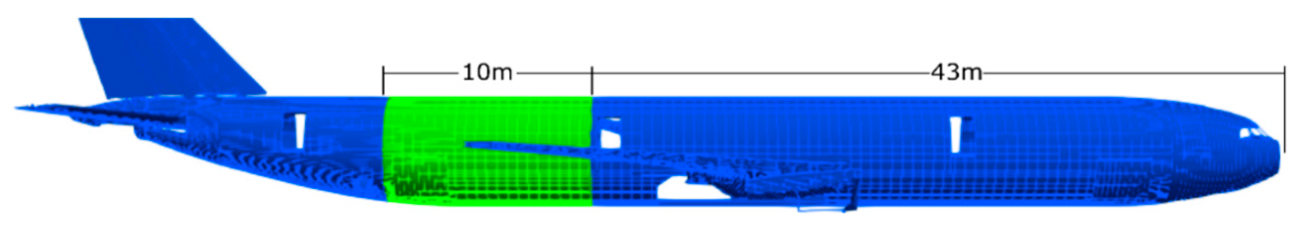
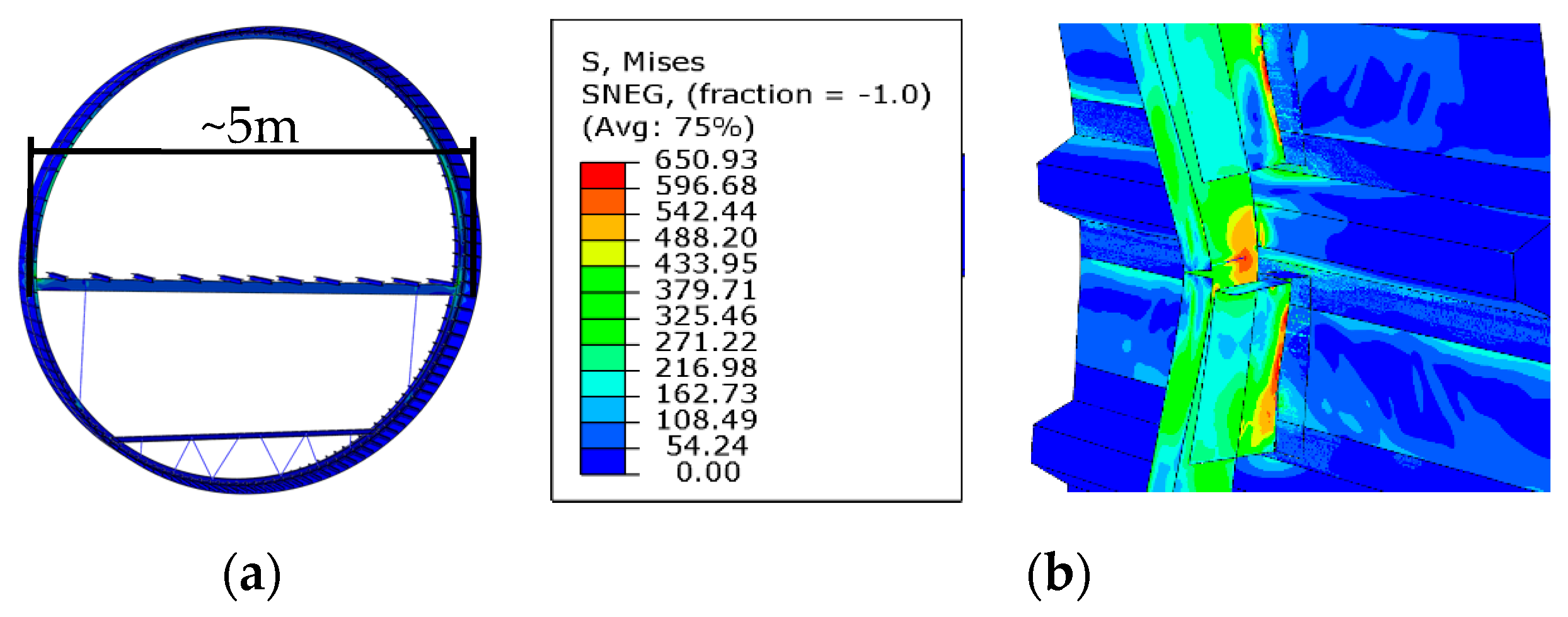
3.2.1. Global FE-Model

Preliminary ditching simulations with a rigid aircraft similar to the A350 show that an approximately 10 m long section of the rear fuselage is subjected to water loads during the impact phase of a ditching event. The relevant section is shown in Figure 9. Though only a small part of the fuselage is subjected to the hydrodynamic impact loads, the whole aircraft needs to be structurally modelled to capture the overall dynamics during impact. If structural damage occurs, it is expected to be limited to the green region.

To capture the overall aircraft dynamics outside the green region, a global FEM model (GFEM) based on the XRF-1, an Airbus large transport aircraft of the eXternal Research Forum (XRF), is used. Stringers and frames are modelled as rods and beams on a skin modelled as shells, whereas masses are defined as point masses which are assigned to whole fuselage sections. The total number of degrees of freedom in the model amounts to approximately 300k.

3.2.2. Fuselage Crash Simulations

The majority of the available methods to simulate fuselage damage under crash conditions primarily address barrel drop tests on solid ground. Two distinct numerical approaches can be found in the literature.

The first approach is to discretize the airframe as a lumped mass-spring-damper system. This leads to small models with only several hundred degrees of freedom. Examples of such an implementation are DRI-KRASH solver described in Reference [13] or a method by Weiß proposed in Reference [38]. Obvious advantages of those approaches are their simplicity of application and reduced computational effort. This allows examining many different configurations and crash scenarios. However, the parameters needed for those models have to be obtained experimentally or from experience. Furthermore, the results need to be carefully reviewed as the range of validity cannot be reliably predicted.

The other approach is the simulation on a high-fidelity level using explicit FE solvers [39]. Although this approach tends to be more accurate, experimental verification still remains an important requirement. Another major disadvantage is the high computational cost. Besides the model size, the computational effort is dependent on the physical time to be simulated as well as the refinement level in the model. Especially the latter can cause problems as the maximum time step size is directly linked to the size of the smallest element in the model. A second disadvantage is that the required degree of granularity in the model needs to be determined. In this context, the term granularity not only refers to the element size but also to the level of structural detail, for instance, if discrete rivets with failure criterions are modelled. For barrel drop tests, suitable degrees of granularity were determined by comparisons between simulations and experiments. However, the question if those results are applicable to the simulation of ditching events still remains unanswered.

If a direct simulation of damage with the explicit FE method is employed, the structural models need to be fine enough to account for relevant damage effects. To illustrate this, the simulation of a breaking frame loaded by a bending moment is shown in Figure 10b. As frames serve as circumferential stiffeners, their failure has the biggest impact on the overall stiffness of the fuselage [38]. The damage is highly localized and the damage region is magnitudes of order smaller compared to the overall aircraft dimensions.

Due to complex damage mechanisms, that are triggered by stability buckling in the inner flange or by plasticity effects, respectively, a very fine mesh is needed to directly simulate the damage. Consequently, a mesh size study is conducted for the case depicted in Figure 10b. The results are summarized in Figure 11, showing the bending angle over the applied momentum for different element edge lengths. The results indicate that very fine meshes are needed to get a reliable ultimate momentum. In addition, the post-failure stiffness is very dependent on the mesh size, as many damage effects are very small in scale.

The complete ditching event is expected to have a duration of several seconds and, as the computation effort grows with the simulated time, an FE model that accounts for structural damage within the region relevant for ditching by using a sufficiently fine mesh while simultaneously capturing the whole aircraft is not feasible. Therefore, the authors suggest using a multiscale model for the structural simulation.

3.2.3. Multiscale Model for Ditching Simulation

To model the section of the aircraft relevant for ditching, a combination of the two methods outlined in Section 3.2.2 is used. The green section shown in Figure 9 is modelled using an FE discretization with an element size between 15 and 20 mm. The water loads are applied to the fuselage skin. To allow the correct simulation of the load paths within the model, stringers, clips and frames are modelled as shells. The resulting model has approximately 6M degrees of freedom and, therefore, can be handled by commercial explicit FE solvers. The blue region in Figure 9 resembles the GFEM-model. Both parts of the model are connected by multi-point-constraints.

In addition to the refined mesh, a better approximation of the mass distribution is needed as inertia forces are important for the loading state during highly dynamic events. The structural masses of the refined region are directly incorporated by material densities while passenger and cargo masses are separately modelled. Afterwards, the difference in mass to the original GFEM section is evenly smeared over all elements of the model. In this way, the original mass as well as the overall mass properties of the aircraft, which are essential for the computation of the correct trajectory during ditching, are preserved. Although the moments of inertia in the green section are not preserved exactly, their influence on the overall moment of inertia is relatively small.

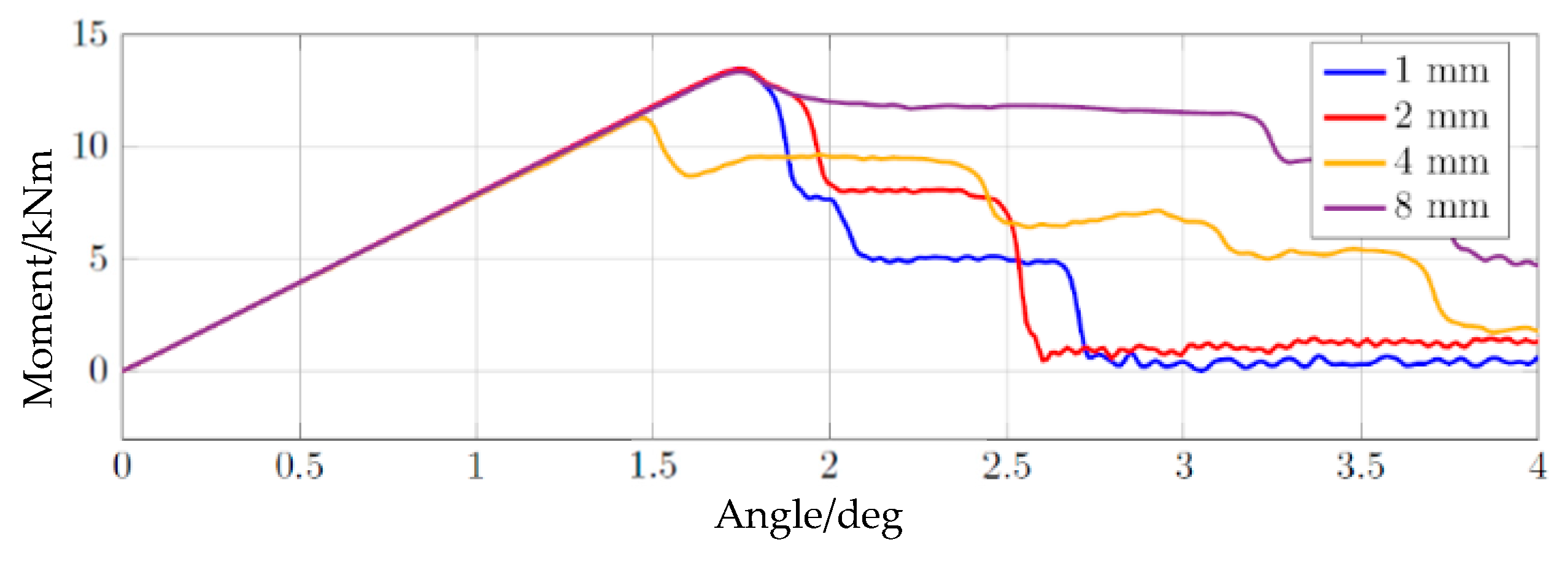
3.2.4. Modelling Damage

At this stage, the structural model is still too coarse to accurately account for damage effects as discussed in Section 3.2.2. Most parts of the structure are subjected to characteristic loading states. The stringers in combination with the skin are for example primarily loaded by longitudinal stresses introduced by bending of the fuselage, whereas the frames keep the fuselage cross sections in shape and are mainly loaded by bending moments and hoop stresses. The clips transfer the loads from the skin to the frame and are therefore subjected to shear stresses. These observations can be used to introduce reduced order models that can capture damage effects using a relatively coarse FE discretization. This approach is called Kinematics Model and was described by Waimer et al. in Reference [13]. For instance, the damage of a frame can be modelled as a non-linear hinge element with the centre of rotation located at the skin. The hinge is closed for uncritical loads and starts to open as soon as the frame starts to break. The moment to opening angle curve is obtained either from experimental results or, as done in his case, by using the results of a detailed FE simulation as shown for example in Figure 11. Due to the highly localized damage, its overall effect on the structural behaviour can be captured by such approaches with sufficient accuracy.

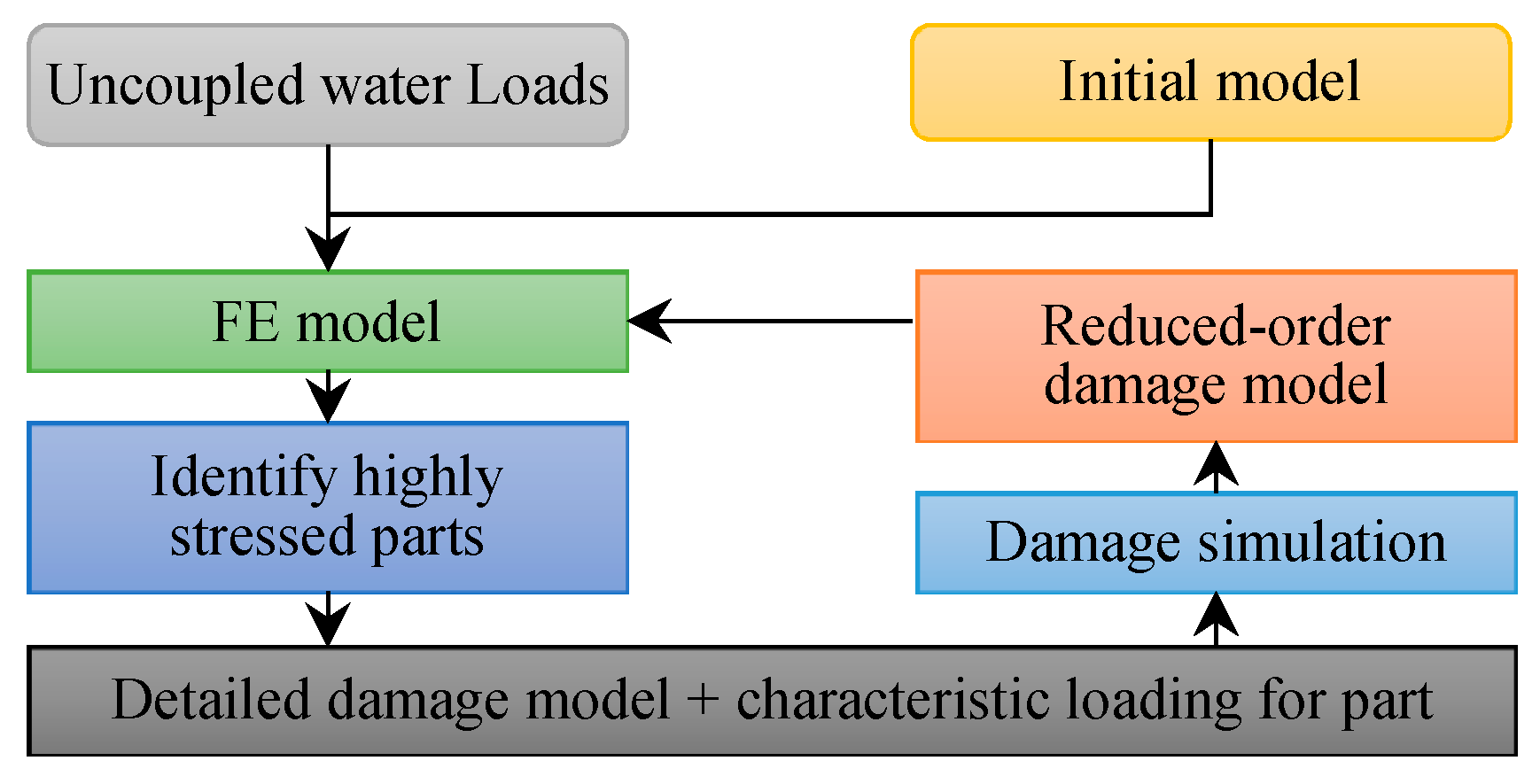
3.2.5. Creating the Multiscale Model

To create a reduced order damage model without having access to full scale ditching experiments, it is necessary to identify locations of the structure where damage might occur as well as the characteristic loading states of the corresponding parts. In addition to the frames, the vertical struts are considered as well as they have a significant influence on the damage characteristics [38]. For the creation of the multiscale model, the iterative process shown in Figure 12 is proposed.

The initial FE model is loaded by water loads obtained from a ditching simulation of a rigid structure with similar outer geometry. Highly stressed regions are identified and the characteristic loading states are extracted. For the identified regions, FE damage models with a high level of granularity are created and loaded with their respective characteristic loading states. Based on the results of the detailed simulations, appropriate surrogate models, that are able to reproduce the kinematics of the damage, are chosen and provided with the calculated load to deformation curve. The surrogate models are then introduced into the fuselage FE model. The procedure is repeated as the occurrence of damage may change the load path of the structure. If no further critical locations are found the iteration process is stopped.

4. Conclusions and Outlook

In this study, a fluid-structure coupling framework suitable for ditching simulations is presented and validated. The partitioning of the computational domain is done by the standard Dirichlet-Neumann approach. It is shown that this framework works well for two-dimensional cases with rigid and deformable structures if an implicit fixed-point iteration scheme is used. However, in the deformable case, this scheme proves to be inefficient for the iterative coupling scheme and even becomes unstable if an explicit structural solver is used together with a simple staggered coupling approach. Those results indicate that carefully designed coupling procedures need to be developed to increase computational efficiency and facilitate the usage of explicit structural solvers in the simulation of ditching problems. In this context, a simple staggered coupling scheme would be favourable but certainly requires partitioning approaches other than standard Dirichlet-Neumann boundary conditions. Possible options include operator-splitting techniques (e.g., [40]), mixed boundary conditions (e.g., [41,42]) or the weak introduction of coupling conditions (e.g., [43]). For full-scale ditching simulations, which include the failure of the structure, the time scales of fluid and structural simulation are expected to differ significantly. Hence, sub-cycling of the structural solver will likely be necessary to keep the computational effort at a manageable amount.

Furthermore, as soon as horizontal speed is introduced and mesh deformation becomes an issue, the overset grid technique is a viable option to allow large movements of the fluid-structure boundary while at the same time preserving the quality of the fluid mesh [44].

The second key point of this study pertains the development of a multiscale structural model of the aircraft fuselage. It is shown that a structural model that on the one hand can capture the overall dynamics of the aircraft and, on the other hand, directly simulate structural damage is not feasible. Due to severe nonlinearities in the structure, explicit time integration is needed. However, simply refining damage relevant regions would lead to impracticable short time steps and very poor overall computational efficiency. A method is presented how the highly localized damage behaviour of aeronautical structures can be incorporated in full-size aircraft models while retaining a model size that can be handled by today‘s computers. This is done by reduced order models that account for the correct kinematics of structural damage and the combination of a GFEM model with a locally refined section of interest. An iterative process is proposed how relevant regions, where reduced order damage models should be placed, can be identified.

References

1. European Aviation Safety Agency. Certification Specifications and Acceptable Means of Compliance for Large Aeroplanes CS-25, Book 1—Certification Specifications, Subpart C, Section CS 25.801—Ditching: CS 25.801. Amendment 22. Available online: https://www.easa.europa.eu/sites/default/files/dfu/CS-25%20Amendment%2022.pdf (accessed on 11 January 2019).
2. Federal Aviation Administration (FAA), Department of Transportation. Code of Federal Regulations, Title 14, Chapter I, Subchapter C, Part 25, Subpart D, Section 25.801—Ditching: 14 CFR 25.801. Available online: https://www.law.cornell.edu/cfr/text/14/25.801 (accessed on 11 January 2019).
3. Siemann, M.H.; Langrand, B. Coupled fluid-structure computational methods for aircraft ditching simulations: Comparison of ALE-FE and SPH-FE approaches. Comput. Struct. 2017, 188, 95–108. [Google Scholar] [CrossRef]
4. Pentecôte, N.; Vigliotti, A. Crashworthiness of helicopters on water: Test and simulation of a full-scale WG30 impacting on water. Int. J. Crashworth. 2003, 8, 559–572. [Google Scholar] [CrossRef]
5. Wernsdorfer, T.; Keller, K.; Climent, H. CN-235-300M Deepwater—Subscale Model, Ditching and Floatation Tests Plan, Issue A; EASA-CASA: Madrid, Spain, 2003. [Google Scholar]
6. Climent, H.; Benitez, L.; Rosich, F.; Rueda, F.; Pentecote, N. Aircraft Ditching Numerical Simulation. In Proceedings of the 25th International Congress of the Aeronautical Sciences, Hamburg, Germany, 3–8 September 2006. [Google Scholar]
7. Keller, A.P. Cavitation Scale Effects—Empirically Found Relations and the Correlation of Cavitation Number and Hydrodynamic Coefficients. In Proceedings of the CAV 2001: Fourth International Symposium on Cavitation, California Institute of Technology, Pasadena, CA, USA, 20–23 June 2001. [Google Scholar]
8. Lindenau, O.; Busch, C.; Streckwall, H.; Bensch, L.; Rung, T. Validation of a transport aircraft ditching simulation tool. In Proceedings of the 6th International KRASH Users’ Seminar (IKUS6), Stuttgart, Germany, 15–17 June 2009. [Google Scholar]
9. Halbout, S.; Vagnot, A.; Markmiller, J. Modelling of water impact during ditching event. Available online: https://dspace-erf.nlr.nl/xmlui/bitstream/handle/20.500.11881/3673/ERF2016_47_S.%20HALBOUT%20_P.pdf?sequence=1 (accessed on 11 January 2019).
10. Anghileri, M.; Castelletti, L.-M.L.; Francesconi, E.; Milanese, A.; Pittofrati, M. Survey of numerical approaches to analyse the behavior of a composite skin panel during a water impact. Int. J. Impact Eng. 2014, 63, 43–51. [Google Scholar] [CrossRef]
11. Bisagni, C.; Pigazzini, M.S. Modelling strategies for numerical simulation of aircraft ditching. Int. J. Crashworth. 2018, 23, 377–394. [Google Scholar] [CrossRef]
12. Iafrati, A.; Grizzi, S.; Siemann, M.H.; Benítez Montañés, L. High-speed ditching of a flat plate: Experimental data and uncertainty assessment. J. Fluids Struct. 2015, 55, 501–525. [Google Scholar] [CrossRef]
13. Waimer, M.; Kohlgrüber, D.; Hachenberg, D.; Voggenreiter, H. The Kinematics Model—A Numerical Method for the Development of a Crashworthy Composite Fuselage Design of Transport Aircraft. In Proceedings of the Sixth Triennial International Aircraft Fire and Cabin Safety Research Conference, Atlantic City, NJ, USA, 25–28 October 2010. [Google Scholar]
14. Reinhard, M.; Korobkin, A.A.; Cooker, M.J. Water entry of a flat elastic plate at high horizontal speed. J. Fluid Mech. 2013, 724, 123–153. [Google Scholar] [CrossRef] [Green Version]
15. Newman, J.M. Marine Hydrodynamics; MIT Press: Cambridge, MA, USA, 1977. [Google Scholar]
16. Le Tallec, P.; Mouro, J. Fluid structure interaction with large structural displacements. Comput. Methods Appl. Mech. Eng. 2001, 190, 3039–3067. [Google Scholar] [CrossRef]
17. Causin, P.; Gerbeau, J.F.; Nobile, F. Added-mass effect in the design of partitioned algorithms for fluid–structure problems. Comput. Methods Appl. Mech. Eng. 2005, 194, 4506–4527. [Google Scholar] [CrossRef] [Green Version]
18. Förster, C.; Wall, W.A.; Ramm, E. Artificial added mass instabilities in sequential staggered coupling of nonlinear structures and incompressible viscous flows. Comput. Methods Appl. Mech. Eng. 2007, 196, 1278–1293. [Google Scholar] [CrossRef]
19. Küttler, U.; Wall, W.A. Fixed-point fluid–structure interaction solvers with dynamic relaxation. Comput. Mech. 2008, 43, 61–72. [Google Scholar] [CrossRef]
20. Küttler, U.; Gee, M.; Förster, C.; Comerford, A.; Wall, W.A. Coupling strategies for biomedical fluid–structure interaction problems. Int. J. Numer. Methods Biomech. Eng. 2010, 26, 305–321. [Google Scholar] [CrossRef]
21. Ortiz, R.; Charles, J.L.; Sobry, J.F. Structural loading of a complete aircraft under realistic crash conditions: Generation of a load database for passenger safety and innovative design. In Proceedings of the 24th International Congress of the Aeronautical Sciences, Yokohama, Japan, 29 August–3 September 2004. [Google Scholar]
22. Kohlgruber, D.; Vigliotti, A.; Weissberg, V.; Bartosch, H. Numerical simulation of a composite helicopter sub-floor structure subjected to water impact. In Proceedings of the 60th Annual Forum of the American Helicopter Society, Baltimore, MD, USA, 7–10 June 2004; pp. 7–10. [Google Scholar]
23. Groenenboom, P.H.; Campbell, J.; Benítez Montañés, L.; Siemann, M.H. Innovative SPH methods for aircraft ditching. In Proceedings of the 11th WCCM/5th ECCM, Barcelona, Spain, 20–25 July 2014. [Google Scholar]
24. Smith, A.G.; Warren, C.H.E.; Wright, D.F. Investigations of the Behaviour of Aircraft When Making a Forced Landing on Water (Ditching); Her Majesty’s Stationery Office: London, UK, 1957. [Google Scholar]
25. Kowollik, D.; Tini, V.; Reese, S.; Haupt, M. 3D fluid-structure interaction analysis of a typical liquid rocket engine cycle based on a novel viscoplastic damage model. Int. J. Numer. Methods Eng. 2013, 94, 1165–1190. [Google Scholar] [CrossRef]
26. Lindhorst, K.; Haupt, M.C.; Horst, P. Reduced-order modelling of non-linear, transient aerodynamics of the HIRENASD wing. Aeronaut. J. 2016, 120, 601–626. [Google Scholar] [CrossRef]
27. Sommerwerk, K.; Haupt, M.C. Design analysis and sizing of a circulation controlled CFRP wing with Coandǎ flaps via CFD–CSM coupling. CEAS Aeronaut. J. 2014, 5, 95–108. [Google Scholar] [CrossRef]
28. Haupt, M.; Niesner, R.; Unger, R.; Horst, P. Computational Aero-Structural Coupling for Hypersonic Applications. In Proceedings of the 9th AIAA/ASME Joint Thermophysics and Heat Transfer Conference, San Francisco, CA, USA, 5–8 June 2006; American Institute of Aeronautics and Astronautics: Reston, VA, USA, 2006; p. 95. [Google Scholar]
29. Müller, M.; Haupt, M.; Horst, P. Socket-Based Coupling of OpenFOAM and Abaqus to Simulate Vertical Water Entry of Rigid and Deformable Structures. In Proceedings of the 6th ESI OpenFOAM User Conference 2018, Hamburg, Germany, 23–25 October 2018. [Google Scholar]
30. Mok, D.P.; Wall, W.A.; Ramm, E. Accelerated iterative substructuring schemes for instationary fluid-structure interaction. Comput. Fluid Solid Mech. 2001, 2, 1325–1328. [Google Scholar]
31. Greenhow, M.; Lin, W.M. Nonlinear-Free Surface Effects: Experiments and Theory; Massachusetts Institute of Technology Cambridge: Cambridge, MA, USA, 1983. [Google Scholar]
32. Deshpande, S.S.; Anumolu, L.; Trujillo, M.F. Evaluating the performance of the two-phase flow solver interFoam. Comput. Sci. Discov. 2012, 5, 14016. [Google Scholar] [CrossRef] [Green Version]
33. Roenby, J.; Bredmose, H.; Jasak, H. A computational method for sharp interface advection. R. Soc. Open Sci. 2016, 3, 160405. [Google Scholar] [CrossRef]
34. Arai, M.; Miyauchi, T. Numerical Simulation of the Water Impact on Cylindrical Shells Considering Fluid-Structure Interaction. J. Soc. Nav. Archit. Jpn. 1997, 1997, 827–835. [Google Scholar] [CrossRef]
35. Sun, H.; Faltinsen, O.M. Water impact of horizontal circular cylinders and cylindrical shells. Appl. Ocean Res. 2006, 28, 299–311. [Google Scholar] [CrossRef]
36. Ionina, M.F.; Korobkin, A.A. Water Impact on Cylindrical Shell. In Proceedings of the 14th International Workshop on Water Waves and Floating Bodies, Port Huron, MI, USA, 11–14 April 1999. [Google Scholar]
37. Wagner, H. Über Stoss-und Gleitvorgänge an der Oberfläche von Flüssigkeiten. Z. Angew. Math. Mech. 1932, 12, 193–235. [Google Scholar] [CrossRef]
38. Weiß, L. Initial Design of Crashworthy Composite Structures. Ph.D. Thesis, Technischen Universität Carolo-Wilhelmina, Braunschweig, Germany, 2016. [Google Scholar]
39. Byar, A. A Crashworthiness Study of a Boeing 737 Fuselage Section. Ph.D. Thesis, Drexel University, Philadelphia, PA, USA, 2003. [Google Scholar]
40. Guidoboni, G.; Glowinski, R.; Cavallini, N.; Canic, S. Stable loosely-coupled-type algorithm for fluid–structure interaction in blood flow. J. Comput. Phys. 2009, 228, 6916–6937. [Google Scholar] [CrossRef]
41. Li, L.; Henshaw, W.D.; Banks, J.W.; Schwendeman, D.W.; Main, A. A stable partitioned FSI algorithm for incompressible flow and deforming beams. J. Comput. Phys. 2016, 312, 272–306. [Google Scholar] [CrossRef] [Green Version]
42. Badia, S.; Quaini, A.; Quarteroni, A. Modular vs. non-modular preconditioners for fluid–structure systems with large added-mass effect. Comput. Methods Appl. Mech. Eng. 2008, 197, 4216–4232. [Google Scholar] [CrossRef] [Green Version]
43. Burman, E.; Fernández, M.A. Explicit strategies for incompressible fluid-structure interaction problems: Nitsche type mortaring versus Robin-Robin coupling. Int. J. Numer. Methods Eng. 2014, 97, 739–758. [Google Scholar] [CrossRef]
44. Steger, J.L.; Dougherty, F.C.; Benek, J.A. A chimera grid scheme. [Multiple overset body-conforming mesh system for finite difference adaptation to complex aircraft configurations]. Advances in grid generation. In Proceedings of the Applied Mechanics, Bioengineering, and Fluids Engineering Conference, Houston, TX, USA, 20–22 June 1983; (A84-11576 02-64). American Society of Mechanical Engineers: New York, NY, USA, 1983; pp. 59–69. [Google Scholar]
Figure 1. Coupling environment ifls (see [25,26,27]).
Aerospace 06 00010 g001
Figure 2. Solution procedure for time level t n .
Aerospace 06 00010 g002
Figure 3. Drop test of rigid cylinder: (a) Schematic representation of drop test; (b) Section of the fluid mesh (mesh02).
Aerospace 06 00010 g003
Figure 4. Drop test of rigid cylinder: (a) Schematic representation of drop test; (b) Results from drop test of rigid cylinder, experimental results from [31].
Aerospace 06 00010 g004
Figure 5. Stages of water impact of rigid cylinder.
Aerospace 06 00010 g005
Figure 6. Section of the structural mesh of deformable cylindrical shell.
Aerospace 06 00010 g006
Figure 7. Strain response of deformable cylinder (reference data from [34,35]): (a) Comparison of different mesh configurations using ρ s = ρ s , 2 ; (b) Comparison of different structural densities.
Aerospace 06 00010 g007
Figure 8. Iterations needed per time step during impact.
Aerospace 06 00010 g008
Figure 9. Relevant structural region (highlighted in green) of an A350-type aircraft.
Aerospace 06 00010 g009
Figure 10. Structural model in detail: (a) Slice of the medium-detailed FE model (green region); (b) Damage FE model of a frame subjected to a bending moment.
Aerospace 06 00010 g010
Figure 11. Results of the model in Figure 10b with different element side lengths.
Aerospace 06 00010 g011
Figure 12. The iterative process of model creation.
Aerospace 06 00010 g012