A High-Precision Adaptive Sequential Convex Programming Method for Non-Coplanar Transfer Trajectory Optimization in Constellation Aggregation

Abstract

With the development of constellations and satellite chains, trajectory planning for constellation satellites has gradually attracted research attention. To address the infeasibility issues of trapezoidal sequential convex programming (T-SCP) in this strong non-convexity problem, this paper proposes high-precision adaptive SCP based on the Hermite Simpson method for Low-Earth-Orbit (LEO) constellation aggregation and aimed at enhanced local reconnaissance with practical constraints, including collision avoidance. The method introduces an adaptive trust region and slack variables, which avoid convergence failures due to strong nonlinearity or large state variations over long distances and accelerate the convergence rate. Furthermore, a third-order accurate Hermite Simpson method is adopted along with a adaptive iterative collision warning mechanism, improving accuracy while reducing computational cost. Simulation results demonstrate that the proposed method improves computational efficiency by 6% and 21% compared with the T-SCP and pseudospectral method, respectively. When the number of discrete nodes is 50, it achieves position errors of 284.7 m and velocity errors of 0.33 m/s, and these errors are far lower than those of T-SCP. Monte Carlo simulations across 10,000 scenarios validate the robustness of the proposed method with a 91% overall success rate and 100% for LEO.

1. Introduction

In 2024, SpaceX initiated a large-scale deorbit of early-generation Starlink satellites after identifying potential hardware failures, demonstrating the critical importance of efficient trajectory planning for constellation management. By 2025, Starlink satellites performed approximately 300,000 collision avoidance maneuvers annually, highlighting the growing complexity of multi-spacecraft coordination in increasingly congested orbital environments. These developments underscore the urgent need for robust, computationally efficient trajectory optimization methods capable of handling large-scale satellite clusters with stringent safety requirements.

Spacecraft cluster orbit transfer optimization involves coordinated orbital maneuvers of multiple spacecraft subject to dynamic constraints, collision avoidance constraints, and fuel limitations. Current research primarily focuses on cluster reconfiguration and formation flying in the coordinate frames, where substantial progress has been made in relative motion modeling, cooperative collision avoidance, and formation maintenance. However, for long-range orbit transfers, existing studies are mostly based on the Lambert transfer scheme [1] and employ low-thrust electric propulsion strategies. The former, despite its analytical tractability and computational efficiency, lacks flexibility and optimality in scenarios with multiple constraints, continuous thrust or variable terminal time. The latter, while offering high specific impulse and superior propulsion efficiency, presents trajectory optimization challenges due to strong nonlinearity, multiple variables, and long-time-scale coupling issues, with existing solution methods still facing difficulties in convergence and global optimality. Therefore, research into efficient trajectory optimization methods for long-distance orbital transfers holds significant theoretical importance and engineering value. This work will contribute to deep space exploration, on-orbit servicing, and constellation deployment missions. Research on trajectory optimization is now well-established. Direct methods solve optimal control problems by transforming them into nonlinear programming (NLP) problems through discretization of control and state variables, utilizing algorithms such as sequential quadratic programming (SQP) and interior point methods (IPM). Sequential quadratic programming can effectively solve complex trajectory optimization problems [2], yielding high-precision globally optimal solutions. Pseudospectral methods, as a class of direct methods, approximate state and control variables through global polynomial interpolation. Common pseudospectral approaches include the Legendre–Gauss–Lobatto (LGL) pseudospectral method [3], Chebyshev pseudospectral method, Gauss pseudospectral method, and hp pseudospectral method [4]; they discretize states and controls into global interpolation polynomials at collocation points of orthogonal polynomials. Pseudospectral methods achieve high accuracy with fewer discretization points and converge rapidly. However, they are sensitive to initial guesses, and for large-scale, long-duration orbit transfers, excessive discretization points lead to significantly increased computational burden. Indirect methods are based on Pontryagin’s minimum principle, which transforms optimal control problems into two-point boundary value problems (TPBVP) by deriving necessary conditions. This approach possesses theoretical precision and the advantage of high-accuracy solutions, providing theoretical guarantees of optimality [5]. Indirect methods have demonstrated excellent performance in low-thrust orbit transfer and optimal impulsive maneuver problems. However, indirect methods are also extremely sensitive to initial guesses and require deriving complex costate equations and transversality conditions. For highly nonlinear spacecraft cluster problems, indirect methods are often difficult to solve and exhibit numerical instability issues.

These algorithms possess strong global search capabilities and do not rely on gradient information, making them suitable for high-dimensional, nonlinear, multi-modal global optimization problems. Intelligent algorithms have advantages in handling multi-objective optimization and non-convex problems, but they typically underperform gradient-based methods in terms of solution accuracy and convergence speed. In orbit transfer optimization, they are commonly used to provide initial guesses or perform multi-objective optimization. Ref. [6] trained neural networks to solve low-thrust, multi-revolution, long-period transfer orbit optimization problems. They employ random search to optimize network hyperparameters and effectively improve training efficiency. The drawbacks are that it is computationally intensive and it is difficult to guarantee the feasibility and optimality of the solution. Ref. [7] utilized particle swarm optimization to generate a series of initial guesses satisfying boundary conditions for gradient-based algorithms. For impulsive thrust transfers, ref. [1] proposed an efficient multi-revolution Lambert transfer solver capable of computing all Lambert transfer orbit solutions in all cases. The Lambert problem determines an orbit between two points from given position vectors and transfer time. In the multi-revolution case, there are multiple feasible orbits, and the solution process must additionally select the optimal number of revolutions along with the orbital parameters. Lambert solution methods typically assume impulsive thrust action, thus requiring further treatment for spacecraft with continuous low-thrust. Ref. [8] applied adaptive dynamic programming to address the robust control problem of hypersonic vehicles. Ref. [9] comparatively evaluated the performance of Timed Elastic Band (TEB) and Model Predictive Control (MPC) as local planners in robotics and demonstrated that MPC exhibits superior path tracking performance.

A more effective approach is convex optimization, which transforms the original non-convex problem into a convex optimization problem, offering the advantages of global optimality guarantees and polynomial-time complexity. The key to convex optimization methods lies in convexification processing, including constraint relaxation, variable substitution, and linearization. However, direct application of convex optimization is challenging for orbit transfer problems involving nonlinear dynamics and non-convex constraints; thus, it is often combined with other methods. Sequential convex programming (SCP) methods [10] are commonly employed. The fundamental idea is to linearize the non-convex dynamics and constraints at the current iteration point, approximating the original problem as a convex optimization problem and iteratively solving this convex subproblem until convergence. This algorithm possesses guarantees of global convergence and superlinear convergence rates [11] and has been widely applied to various mission scenarios, including low-thrust spacecraft trajectory planning, rendezvous and docking, and interplanetary transfers. For instance, ref. [12] applied SCP to fuel-optimal low-thrust Earth–Mars transfer problems, achieving problem convexification through variable substitution and constraint relaxation, and obtained optimization results comparable to GPOPS-II using interior point methods. Ref. [13] further improved the variable substitution strategy by proposing an SCP method without introducing additional relaxation variables, effectively reducing the number of iterations and improving convergence speed. Furthermore, SCP can also address spacecraft cluster collision avoidance orbit transfer problems. Ref. [14] introduced linearized minimum separation distance constraints to transform the non-convex collision avoidance constraints into convex linear inequality constraints, enabling efficient solution of cluster cooperative orbit optimization problems through SCP.

Despite the significant advantages of SCP in handling non-convex optimal control problems, it still faces numerous challenges and limitations in practical applications. The first challenge is the infeasibility problem: even if the original problem has a feasible solution, the convex subproblems generated from decomposition may not have feasible solutions. This is primarily due to the linearization of dynamic equations and convexification of non-convex constraints. This infeasibility problem is more prominent when using SCP to solve long-range time-optimal problems with stronger non-convexity in dynamic models and constraints. Specifically, linearization introduces approximation errors. For strongly nonlinear dynamics and constraint conditions, linearization approximations may significantly deviate from the true constraints, resulting in final solutions that do not satisfy the original problem’s constraints. To improve solution feasibility, multiple iterative corrections or higher-order approximations are typically required. Ref. [15] proposed the Hermite–Simpson method to improve discretization accuracy with improved adaptive meshing, achieving higher computational efficiency. However, the applicable scenarios are limited to two-dimensional time-optimal and three-dimensional fuel-optimal low-thrust orbit transfer problems, without analysis of more complex three-dimensional time-optimal problems. Meanwhile, higher accuracy implies increased computational cost. For equality constraints and non-convex constraints, convexification must first be performed, and this process also involves convexification loss. Ref. [16] introduced relaxation variables to achieve lossless convexification for highly non-convex problems in solar sail trajectory optimization control variables. Ref. [17] analyzed various non-convex variables and constraints in different optimization problems and provided general convexification methods. Lossless convexification techniques can partially address the infeasibility problem. Additionally, infeasibility can be prevented by introducing virtual control and a trust region within the algorithm [18,19]. Virtual controls ensure subproblem feasibility, while trust regions limit the step size of each iteration to ensure the validity of linear approximations. The results demonstrated higher convergence efficiency compared to SQP and general IPM solvers. Although introducing virtual controls can mitigate the infeasibility problem to some extent, excessively large virtual control terms may reduce the physical executability of the solution, requiring optimization with virtual controls as penalty terms.

The convergence speed is related to the initial guess, trust region update strategy, and the solution accuracy of convex subproblems. For highly nonlinear spacecraft cluster problems, especially when considering complex constraints and perturbations, the algorithm may exhibit oscillations or become trapped in locally infeasible regions, making it difficult to converge to a feasible solution [20]. Although improvements have been made compared to indirect methods, the quality of the initial trajectory guess still affects algorithm performance. An inappropriate choice may lead to convergence difficulties or cause the solution to converge to a local optimum. Particularly when dealing with multi-revolution transfers and complex constraints, the initial guess becomes a critical challenge. Although convex subproblems can be rapidly solved by using mature interior point methods, the computational efficiency is limited in practical on-orbit applications. The number of iterations, the trust-region update strategy, and the efficiency of subproblem solving all affect the computational efficiency of SCP. Moreover, SCP methods are primarily designed for single-objective optimization problems and face challenges when dealing with multi-objective optimization, such as simultaneously optimizing fuel consumption and transfer time. While the weighting method can convert the problem into a single-objective formulation, challenges still persist in choosing appropriate weights and exploring the Pareto front [21].

This paper presents a sequential convex programming framework featuring an adaptive trust-region update with slack variables. A dynamically consistent orbital-element interpolation provides a feasible initial guess, preventing infeasibility in convex subproblems. The Hermite–Simpson method enhances discrete accuracy to address long-distance transfer challenges, while a collision warning mechanism reduces computation and improves efficiency. Unlike most existing methods that only validate scenarios within the same orbital plane, the simulations in this paper cover two typical mission types: same-plane and adjacent-plane orbital aggregation. The results demonstrate that the proposed strategy converges stably under both configurations, significantly extending the applicability of sequential convex programming to multi-plane orbital aggregation problems.

The main contributions of this paper are summarized as follows: A novel adaptive trust region update strategy combined with slack variable relaxation is proposed to ensure linearization validity and provide a feasibility margin, which prevents convergence failures caused by strong nonlinearities or large state variations and accelerates convergence. The Hermite–Simpson collocation method with third-order accuracy is employed to reduce linearization error accumulation over long transfer trajectories, and the collision early warning mechanism is adopted, which activates constraints only within spacecraft with a potential collision risk, thus reducing active constraints and improving computational efficiency while preserving safety. Comprehensive numerical simulations are conducted covering both same-plane and adjacent-plane orbital aggregation scenarios. While most existing studies only validate within the same orbital plane, this work demonstrates that the proposed method converges stably under both configurations, significantly extending the applicability of sequential convex programming to more general multi-plane orbital transfer problems.

The remainder of this paper is organized as follows. Section 2 presents the problem formulation, including the spacecraft dynamics model with J2 perturbation and atmospheric drag, and the time-optimal trajectory optimization problem formulation with normalized time transformation. Section 3 formulates the multi-spacecraft cluster optimal control problem, including the optimization variables, dynamics constraints using Hermite–Simpson collocation, boundary conditions, control constraints, and collision avoidance constraints with the early warning mechanism. Section 4 provides comprehensive numerical simulation results, comparing the proposed method with trapezoidal collocation and pseudospectral methods. Finally, Section 5 concludes the paper with a summary of findings and perspectives on future research directions.

2. Problem Formulation

2.1. Kinematic Model

The kinematic model is formulated in the Earth-Centered Inertial (ECI) coordinate system. The ECI coordinate system is Earth-centered and inertial, with its origin at the geocenter. The fundamental plane is the Earth’s equatorial plane. The X-axis points toward the vernal equinox, the Z-axis points toward the North Celestial Pole, and the Y-axis completes the right-handed orthogonal system, pointing 90° east of the vernal equinox in the equatorial plane.

In the ECI coordinate system, the motion of a spacecraft is governed by multiple forces including gravitational attraction, perturbations, and thrust. The equation of motion can be expressed as:

$$\ddot{\mathit{r}}=-{\displaystyle \frac{\mu }{r^3}}\mathit{r}+{\mathit{a}}_{J2}+{\mathit{a}}_{drag}+{\displaystyle \frac{1}{m}}\mathit{u}$$

(1)

where $\mathit{r}={[x,y,z]}^T$ is the spacecraft position vector with components along the x, y, and z axes of the ECI frame, $r={\parallel \mathit{r}\parallel }_2$ is the geocentric distance, $\mu =3.986\times {10}^{14}$ m³/s² is Earth’s gravitational parameter, ${\mathit{a}}_{J2}$ represents the J2 perturbation acceleration due to Earth’s oblateness, ${\mathit{a}}_{drag}$ denotes the atmospheric drag acceleration, m is the spacecraft mass, and $\mathit{u}$ is the thrust vector.

The trajectory optimization problem employs the state vector $\mathit{x}={[{\mathit{r}}^T,{\mathit{v}}^T,m]}^T\in {\mathbb{R}}^7$, comprising spacecraft position, velocity, and mass. The equations of motion can be expressed compactly in state-space form:

$$\dot{\mathit{x}}=\mathit{f}(\mathit{x},\mathit{u},t)=\left[\begin{array}{c}\mathit{v}\\ -{\displaystyle \frac{\mu }{r^3}}\mathit{r}+{\mathit{a}}_{J2}+{\mathit{a}}_{drag}+{\displaystyle \frac{1}{m}}\mathit{u}\\ -{\displaystyle \frac{{\parallel \mathit{u}\parallel }_2}{g_0{I}_{sp}}}\end{array}\right]$$

(2)

where $g_0=9.80665$ m/s² is the standard gravitational acceleration at sea level, and $I_{sp}$ is the propulsion system specific impulse in seconds. The mass rate equation indicates that spacecraft mass decreases proportionally to thrust magnitude, with the proportionality constant determined by specific impulse.

2.2. Time-Optimal Problem

In time-optimal trajectory optimization, the final time $t_f$ is an unknown variable requiring optimization alongside the trajectory, which increases the non-convexity of the dynamic constraints. To address this, a normalized time variable $\tau$ is introduced, defined as:

$$\tau ={\displaystyle \frac{t}{\sigma }},\tau \in [0,1]$$

(3)

where $\sigma =t_f$ is the time scaling factor representing total transfer time. This transformation maps the physical time interval $[0,t_f]$ to the fixed normalized interval $[0,1]$, enabling problem formulation on a fixed domain.

The time derivative with respect to normalized time $\tau$ becomes:

$${\displaystyle \frac{\mathrm{d}\mathit{x}}{\mathrm{d}\tau }}={\displaystyle \frac{\mathrm{d}\mathit{x}}{\mathrm{d}t}}·{\displaystyle \frac{\mathrm{d}t}{\mathrm{d}\tau }}=\sigma \dot{\mathit{x}}$$

(4)

This relationship indicates that the state derivative in normalized time is scaled by $\sigma$. Consequently, the transformed dynamics become:

$${\mathit{x}}^{\prime }=\sigma \mathit{f}(\mathit{x},\mathit{u},t)\triangleq \mathit{F}(\mathit{x},\mathit{u},\sigma )$$

(5)

where ${\mathit{x}}^{\prime }=\mathrm{d}\mathit{x}/\mathrm{d}\tau$ denotes the derivative with respect to normalized time. The transformed dynamics $\mathit{F}$ explicitly depend on $\sigma$, which becomes an additional optimization variable.

To apply convex optimization techniques, the transformed dynamics are linearized around a reference trajectory $(\overline{\mathit{x}},\overline{\mathit{u}},\overline{\sigma })$ obtained from the previous SCP iteration or an initial guess. The first-order Taylor expansion yields:

$${\mathit{x}}^{\prime }\approx \overline{\sigma }\mathit{f}(\overline{\mathit{x}},\overline{\mathit{u}})+\overline{\sigma }\mathit{A}(\mathit{x}-\overline{\mathit{x}})+\overline{\sigma }\mathit{B}(\mathit{u}-\overline{\mathit{u}})+\mathit{f}(\overline{\mathit{x}},\overline{\mathit{u}})(\sigma -\overline{\sigma })$$

(6)

where $\mathit{A}=\partial \mathit{f}/\partial \mathit{x}$ and $\mathit{B}=\partial \mathit{f}/\partial \mathit{u}$ are Jacobian matrices evaluated at the reference trajectory.

The Jacobian matrix $\mathit{A}\in {\mathbb{R}}^{7\times 7}$ possesses a specific structure arising from the equations of motion and can be partitioned as:

$$\mathit{A}={\displaystyle \frac{\partial \mathit{f}}{\partial \mathit{x}}}=\left[\begin{array}{ccc}{\mathbf{0}}_{3\times 3}& {\mathit{I}}_{3\times 3}& {\mathbf{0}}_{3\times 1}\\ {\displaystyle \frac{\partial \mathit{a}}{\partial \mathit{r}}}& {\displaystyle \frac{\partial \mathit{a}}{\partial \mathit{v}}}& {\displaystyle \frac{\partial \mathit{a}}{\partial m}}\\ {\mathbf{0}}_{1\times 3}& {\mathbf{0}}_{1\times 3}& 0\end{array}\right]$$

(7)

where $\mathit{a}=-{\displaystyle \frac{\mu }{r^3}}\mathit{r}+{\mathit{a}}_{J2}+{\mathit{a}}_{drag}+{\displaystyle \frac{1}{m}}\mathit{u}$ is the total acceleration, and ${\mathit{I}}_{3\times 3}$ is the $3\times 3$ identity matrix.

The control Jacobian matrix $\mathit{B}\in {\mathbb{R}}^{7\times 3}$ represents the sensitivity of the dynamics to control inputs:

$$\mathit{B}={\displaystyle \frac{\partial \mathit{f}}{\partial \mathit{u}}}=\left[\begin{array}{c}{\mathbf{0}}_{3\times 3}\\ {\displaystyle \frac{1}{m}}{\mathit{I}}_{3\times 3}\\ -{\displaystyle \frac{1}{g_0{I}_{sp}}}{\displaystyle \frac{{\mathit{u}}^T}{{\parallel \mathit{u}\parallel }_2}}\end{array}\right]$$

(8)

2.3. Hermite–Simpson Discretization and Convexation

Beyond dynamics linearization, converting the non-convex optimization problem into a finite-dimensional convex parameter optimization requires discretization. This step critically impacts computational time and solution accuracy for time-continuous optimal control problems. The trajectory is discretized into N nodes over the normalized time interval $\tau \in [0,1]$:

$${\tau }_k={\displaystyle \frac{k}{N}},k=0,1,\dots ,N$$

(9)

where the normalized time step is $\Delta \tau =1/N$.

Traditional sequential convex programming employs uniform mesh discretization techniques such as trapezoidal methods. Achieving higher accuracy with these approaches requires denser uniform mesh points, significantly increasing optimization variables and reducing computational efficiency. The error accumulation of the trapezoidal method leads to the infeasibility of the convex subproblem.

This paper employs the Hermite–Simpson discretization method, providing third-order accuracy while maintaining computational efficiency. This method balances solution accuracy and computational cost, making it particularly suitable for long-duration orbit transfers where numerical errors accumulate significantly. Derived from Simpson’s quadrature rule, it approximates the integral of the state derivative over each interval $[{\tau }_k,{\tau }_{k+1}]$ via a quadratic polynomial that matches the dynamics at both endpoints and the midpoint. This allows using fewer discretization nodes while achieving the same accuracy as the trapezoidal rule with more nodes, potentially reducing overall computational time despite the increased cost per interval.

Let $({\overline{\mathit{x}}}_k,{\overline{\mathit{u}}}_k,\overline{\sigma })$ denote the reference trajectory at node k. The linearized dynamics at each collocation point can be computed according to Equation (6) as follows.

At node k, the linearized dynamics is:

$${\mathit{F}}_k=\overline{\sigma }{\mathit{f}}_k+\overline{\sigma }{\mathit{A}}_k({\mathit{x}}_k-{\overline{\mathit{x}}}_k)+\overline{\sigma }{\mathit{B}}_k({\mathit{u}}_k-{\overline{\mathit{u}}}_k)+{\mathit{f}}_k(\sigma -\overline{\sigma })$$

(10)

where ${\mathit{f}}_k=\mathit{f}({\overline{\mathit{x}}}_k,{\overline{\mathit{u}}}_k)$ is the nonlinear dynamics at the reference. ${\mathit{A}}_k$ is the state Jacobian at node k according to Equation (7), and ${\mathit{B}}_k$ is the control Jacobian at node k according to Equation (8).

Similarly, at node $k+1$:

$${\mathit{F}}_{k+1}=\overline{\sigma }{\mathit{f}}_{k+1}+\overline{\sigma }{\mathit{A}}_{k+1}({\mathit{x}}_{k+1}-{\overline{\mathit{x}}}_{k+1})+\overline{\sigma }{\mathit{B}}_{k+1}({\mathit{u}}_{k+1}-{\overline{\mathit{u}}}_{k+1})+{\mathit{f}}_{k+1}(\sigma -\overline{\sigma })$$

(11)

For each interval $[{\tau }_k,{\tau }_{k+1}]$ with normalized time step $\Delta \tau =1/N$, the Hermite–Simpson method introduces a collocation point at the midpoint ${\tau }_{k+1/2}=({\tau }_k+{\tau }_{k+1})/2$. The control at this midpoint is estimated using a cubic Hermite interpolant:

$${\overline{\mathit{u}}}_{k+1/2}={\displaystyle \frac{1}{2}}({\overline{\mathit{u}}}_k+{\overline{\mathit{u}}}_{k+1})$$

(12)

The estimated midpoint state for the optimization is computed using the linearized dynamics:

$${\overline{\mathit{x}}}_{k+1/2}={\displaystyle \frac{1}{2}}({\mathit{x}}_k+{\mathit{x}}_{k+1})+{\displaystyle \frac{\Delta \tau }{8}}\left({\mathit{F}}_k-{\mathit{F}}_{k+1}\right)$$

(13)

This formula ensures that the midpoint state is consistent with the linearized dynamics at the endpoints.

This simple interpolation is appropriate when the control profile is piecewise linear or when higher-order control interpolation does not significantly affect solution accuracy.

$$\begin{array}{cc}\hfill {\mathit{F}}_{k+1/2}& =\overline{\sigma }{\mathit{f}}_{k+1/2}+\overline{\sigma }{\mathit{A}}_{k+1/2}({\mathit{x}}_{k+1/2}-{\overline{\mathit{x}}}_{k+1/2})\hfill \\ \hfill & +\overline{\sigma }{\mathit{B}}_{k+1/2}({\mathit{u}}_{k+1/2}-{\overline{\mathit{u}}}_{k+1/2})+{\mathit{f}}_{k+1/2}(\sigma -\overline{\sigma })\hfill \end{array}$$

(14)

The fundamental discretization constraint is derived from Simpson’s integration rule, which states that the integral of a quadratic function over an interval can be exactly computed using the function values at the endpoints and midpoint:

$${\int }_{{\tau }_k}^{{\tau }_{k+1}}{\mathit{x}}^{\prime }\mathrm{d}\tau \approx {\displaystyle \frac{\Delta \tau }{6}}\left({\mathit{F}}_k+4{\mathit{F}}_{k+1/2}+{\mathit{F}}_{k+1}\right)$$

(15)

Moreover, even if the convex problem is feasible, the convex subproblems obtained through decomposition may not be feasible. During the sequential iteration process, infeasibility is likely to cause the algorithm to fail to produce a result. This infeasibility mainly arises from the accumulation of errors due to the linearization of the dynamic equations for long-range transfers. Therefore, slack variables can be introduced into the dynamic equations. Then the Hermite–Simpson discretization constraint with slack variables becomes:

$${\mathit{x}}_{k+1}-{\mathit{x}}_k={\displaystyle \frac{\Delta \tau }{6}}\left({\mathit{F}}_k+4{\mathit{F}}_{k+1/2}+{\mathit{F}}_{k+1}\right)+{\mathit{s}}_k$$

(16)

for $k=0,1,\dots ,N-1$, where ${\mathit{s}}_k\in {\mathbb{R}}^7$ is a virtual control variable used to relax the dynamics constraints and avoid infeasibility, which allows the optimization to find feasible solutions even when the linearization is not perfectly accurate. To ensure the accuracy of the final result, these slack variables need to be as small as possible, so they can be incorporated as part of the objective function.

For high-accuracy trajectory optimization, Hermite–Simpson often achieves equivalent accuracy to the trapezoidal rule using fewer nodes, potentially reducing overall computational time despite increased per-interval cost.

To ensure small slack variables and close dynamics satisfaction, the time-optimal objective function includes a slack penalty:

$$J=\sigma +\lambda {\displaystyle \sum _{k=0}^{N-1}}{\parallel {\mathit{s}}_k\parallel }_1$$

(17)

where $\lambda >0$ is the penalty parameter. The ${\ell }_1$-norm encourages sparse slack vectors and reformulates as linear constraints for SOCP:

$${\parallel {\mathit{s}}_k\parallel }_1\le d_{slk}$$

(18)

where $d_{slk}$ is the relaxation variable upper bound.

Since each iteration relies on previous iteration information, significant inter-iteration discrepancies reduce the reliability of $\mathit{A}$ and $\mathit{B}$ matrices derived from previous $\mathit{x}$ and $\mathit{u}$, compromising optimization results. Therefore, a trust region ensures iterative result reliability.

$$\begin{array}{c}\hfill {\parallel {\mathit{x}}_k-{\overline{\mathit{x}}}_k\parallel }_2\le {\delta }_k,{\parallel {\mathit{u}}_k-{\overline{\mathit{u}}}_k\parallel }_2\le {ϵ}_k,|\sigma -\overline{\sigma }|\le 0.3\overline{\sigma }\end{array}$$

(19)

where ${\delta }_k,{ϵ}_k$ are trust region radii, dynamically adjusted based on optimization convergence behavior. The constraint $|\sigma -\overline{\sigma }|\le 0.3\overline{\sigma }$ limits inter-iteration time scaling factor changes. These constraints prevent excessive state trajectory deviation from the reference, maintaining linearization validity and improving convergence.

Additionally, spacecraft must satisfy position and velocity constraints at initial and terminal times. The initial mass is $m_0$ with no terminal mass constraint. The complete time-optimal trajectory optimization problem with Hermite–Simpson discretization is:

$$\begin{array}{cc}\hfill P1:\underset{\sigma ,\mathit{x},\mathit{u},\mathit{s}}{\min }& \sigma +\lambda {\displaystyle \sum _{k=0}^{N-1}}{\parallel {\mathit{s}}_k\parallel }_1\hfill \end{array}$$

(20)

$$\begin{array}{cc}\hfill \hspace{1em}\hspace{1em}\hspace{1em}\hspace{1em}\hspace{1em}\hspace{1em}\hspace{1em}\hspace{1em}\hspace{1em}\hspace{1em}\hspace{1em}\hspace{1em}\mathrm{s}.\mathrm{t}.& {\mathit{x}}_{k+1}-{\mathit{x}}_k={\displaystyle \frac{\Delta \tau }{6}}\left({\mathit{F}}_k+4{\mathit{F}}_{k+1/2}+{\mathit{F}}_{k+1}\right)+{\mathit{s}}_k\hfill \end{array}$$

(21)

$$\begin{array}{cc}\hfill & \hspace{1em}\hspace{1em}\hspace{1em}\hspace{1em}\hspace{1em}\hspace{1em}\hspace{1em}\hspace{1em}{\parallel {\mathit{u}}_k\parallel }_2\le T_{max},k=0,1,\dots ,N\hfill \end{array}$$

(22)

$$\begin{array}{cc}\hfill & \hspace{1em}\hspace{1em}\hspace{1em}\hspace{1em}\hspace{1em}\hspace{1em}{\mathit{x}}_0={\mathit{x}}_{init},{\mathit{x}}_N={\mathit{x}}_{final}\hfill \end{array}$$

(23)

$$\begin{array}{cc}\hfill & \hspace{1em}\hspace{1em}\hspace{1em}\hspace{1em}{\sigma }_{min}\le \sigma \le {\sigma }_{max}\hfill \end{array}$$

(24)

$$\begin{array}{cc}\hfill & \hspace{1em}\hspace{1em}\hspace{1em}\hspace{1em}\hspace{1em}\hspace{1em}\hspace{1em}\hspace{1em}\hspace{1em}\hspace{1em}\hspace{1em}\hspace{1em}\hspace{1em}\hspace{1em}\hspace{1em}\hspace{1em}\hspace{1em}{\parallel {\mathit{x}}_k-{\overline{\mathit{x}}}_k\parallel }_2\le {\delta }_k,{\parallel {\mathit{u}}_k-{\overline{\mathit{u}}}_k\parallel }_2\le {ϵ}_k,|\sigma -\overline{\sigma }|\le 0.3\overline{\sigma }\hfill \end{array}$$

(25)

3. Multi-Spacecraft Cluster Optimal Control Problem

In multi-spacecraft cluster trajectory optimization, all spacecraft must be optimized simultaneously while satisfying individual dynamics constraints and collective mission requirements. This section formulates the convex optimization problem for a cluster of $N_s$ spacecraft.

3.1. Optimization Variables

The multi-spacecraft optimization decision variables include states, controls, and time scaling factors for all spacecraft:

$$\mathcal{X}={\left\{{\mathit{x}}_k^{\left(i\right)},{\mathit{u}}_k^{\left(i\right)},{\sigma }^{\left(i\right)},{\mathit{s}}_k^{\left(i\right)}\right\}}_{i=1,\dots ,N_s}^{k=0,\dots ,N}$$

(26)

where the superscript $\left(i\right)$ denotes the spacecraft index. Each spacecraft has its own trajectory ${\mathit{x}}^{\left(i\right)}\in {\mathbb{R}}^{7\times (N+1)}$, control history ${\mathit{u}}^{\left(i\right)}\in {\mathbb{R}}^{3\times (N+1)}$, time scaling factor ${\sigma }^{\left(i\right)}$, and dynamics slack variables ${\mathit{s}}^{\left(i\right)}\in {\mathbb{R}}^{7\times N}$.

3.2. Dynamics Constraints

Each spacecraft must satisfy its own dynamics constraints. Using the Hermite–Simpson collocation method, the dynamics constraint for the i-th spacecraft at the k-th node is:

$${\mathit{x}}_{k+1}^{\left(i\right)}-{\mathit{x}}_k^{\left(i\right)}={\displaystyle \frac{\Delta \tau }{6}}\left({\mathit{F}}_k^{\left(i\right)}+4{\mathit{F}}_{k+1/2}^{\left(i\right)}+{\mathit{F}}_{k+1}^{\left(i\right)}\right)+{\mathit{s}}_k^{\left(i\right)},\forall i,\forall k$$

(27)

${\mathit{x}}_k^{\left(i\right)}\in {\mathbb{R}}^7$ is the state vector of the i-th spacecraft at the k-th node, containing position, velocity, and mass. ${\mathit{F}}_k^{\left(i\right)}$ is the linearized dynamics of the i-th spacecraft at the k-th node, computed using the reference trajectory. ${\mathit{F}}_{k+1/2}^{\left(i\right)}$ is the linearized dynamics at the midpoint, estimated using the Hermite interpolant. ${\mathit{s}}_k^{\left(i\right)}\in {\mathbb{R}}^7$ is the slack variable that relaxes the dynamics constraint to handle linearization errors. This constraint enforces the equations of motion at each discretization point for all spacecraft.

3.3. Boundary Constraints

Each spacecraft must satisfy its initial and terminal conditions:

$${\mathit{x}}_0^{\left(i\right)}={\mathit{x}}_{init}^{\left(i\right)},{\mathit{x}}_{1:6,N}^{\left(i\right)}={\mathit{x}}_{final,1:6}^{\left(i\right)},\forall i$$

(28)

where ${\mathit{x}}_{init}^{\left(i\right)}={[{\mathit{r}}_0^{\left(i\right)T},{\mathit{v}}_0^{\left(i\right)T},m_0^{\left(i\right)}]}^T$ is the initial state of the i-th spacecraft, including initial position, velocity, and mass. ${\mathit{x}}_{final,1:6}^{\left(i\right)}={[{\mathit{r}}_f^{\left(i\right)T},{\mathit{v}}_f^{\left(i\right)T}]}^T$ is the target position and velocity for i-th spacecraft. The notation ${\mathit{x}}_{1:6,N}^{\left(i\right)}$ indicates the first 6 components (position and velocity) at the final node N. The terminal mass is not constrained, allowing the optimizer to determine fuel consumption.

3.4. Control Constraints

The thrust magnitude for each spacecraft is limited by:

$${\parallel {\mathit{u}}_k^{\left(i\right)}\parallel }_2\le T_{max}^{\left(i\right)},\forall i,\forall k$$

(29)

where ${\mathit{u}}_k^{\left(i\right)}\in {\mathbb{R}}^3$ is the thrust vector of the i-th spacecraft at the k-th node. $T_{max}^{\left(i\right)}$ is the maximum thrust magnitude for the i-th spacecraft.

3.5. Time Scaling Constraints

The time scaling factor for each spacecraft is bounded:

$${\sigma }_{min}^{\left(i\right)}\le {\sigma }^{\left(i\right)}\le {\sigma }_{max}^{\left(i\right)},\forall i$$

(30)

where ${\sigma }^{\left(i\right)}$ is the time scaling factor for the i-th spacecraft, representing the total transfer time. ${\sigma }_{min}^{\left(i\right)}$ is typically set to a fraction of the cluster’s orbital period to ensure the transfer is not too short. ${\sigma }_{max}^{\left(i\right)}$ is typically set to multiple orbital periods to limit the maximum transfer time.

3.6. Adaptive Trust Region Constraints

In sequential convex optimization, the nonlinear dynamics are linearized around a reference trajectory. However, this linearization is only accurate in a neighborhood of the reference. If the optimization is allowed to deviate too far from the reference, the linearization error becomes significant, potentially leading to divergence or convergence to an infeasible solution.

The trust region strategy addresses this issue by constraining the deviation between the optimized trajectory and the reference trajectory. The trust region radius ${\delta }_{tr}$ defines the maximum allowable deviation:

$${\parallel {\mathit{x}}_k^{\left(i\right)}-{\overline{\mathit{x}}}_k^{\left(i\right)}\parallel }_{\infty }\le {\delta }_k^{\left(i\right)},\forall i,\forall k$$

(31)

The region radius is adaptively adjusted based on linearization quality, measured by dynamics constraint violation. The update strategy is:

$${\delta }_k^{\left(i\right)}=\left\{\begin{array}{cc}\max ({\delta }_k^{\left(i\right)}·0.8,0.01)\hfill & \mathrm{if}dyn\_slk<{10}^{-4}\hfill \\ \min ({\delta }_k^{\left(i\right)}·1.1,1.0)\hfill & \mathrm{if}{10}^{-4}\le dyn\_slk<{10}^{-2}\hfill \\ \max ({\delta }_k^{\left(i\right)}·0.7,0.02)\hfill & \mathrm{if}dyn\_slk\ge {10}^{-2}\hfill \end{array}\right.$$

(32)

The selection of the values and intervals is primarily based on empirical settings. When the dynamic slack is large, the linearization error is significant and the trust region should be reduced to improve the linearization accuracy. When the slack is small, it can be considered that convergence is approaching, and the trust region can be slightly expanded to allow faster progress toward the solution.

When the convex optimization subproblem fails, more aggressive trust region reduction is applied:

$${\delta }_k^{(i+1)}={\delta }_k^{\left(i\right)}·0.5$$

(33)

The algorithm terminates if the trust region radius falls below a critical threshold:

$${\delta }_k^{\left(i\right)}<0.001$$

(34)

The trust region radius is also applied to the control variables:

$${\parallel {\mathit{u}}_k^{\left(i\right)}-{\overline{\mathit{u}}}_k^{\left(i\right)}\parallel }_{\infty }\le {ϵ}_k^{\left(i\right)},\forall i,\forall k$$

(35)

and the transfer time:

$$|{\sigma }^{\left(i\right)}-{\overline{\sigma }}^{\left(i\right)}|\le 0.3·{\overline{\sigma }}^{\left(i\right)},\forall i,\forall k$$

(36)

where ${ϵ}_{tr}$ and ${\eta }_{tr}$ are the control and time trust region radii, respectively. ${\overline{\sigma }}^{\left(i\right)}$ is the reference time scaling factor from the previous iteration. The difference is limited to 30% of the reference value. All of these constraints are designed to prevent large jumps in the estimated transfer time that could cause numerical instability. This constraint limits the change in transfer time to 30% of the current estimate, preventing large jumps that could destabilize the optimization. The 30% bound is chosen empirically to balance convergence speed and stability. This constraint is particularly important for time-optimal problems where $\sigma$ is the objective. These constraints ensure that the linearization approximation remains valid. The trust region radii are adaptively adjusted during iteration: decreased when dynamics slack is large, increased when convergence is smooth.

The adaptive trust region strategy provides several key advantages: The algorithm automatically adjusts the step size based on solution quality, eliminating the need for manual parameter tuning during the optimization process. A large initial trust region allows the optimizer to make significant corrections to a poor initial guess, while the adaptive shrinking ensures convergence once near the solution. The trust region expands when the linearization is accurate, allowing faster progress toward the solution. It shrinks when needed to maintain accuracy, avoiding wasted iterations on divergent steps. Under mild conditions, the trust region method guarantees convergence to a stationary point of the original nonlinear problem.

3.7. Adaptive Iterative Collision Warning Mechanism

For cluster missions requiring collision avoidance, additional constraints are imposed:

$${\parallel {\mathit{r}}_k^{\left(i\right)}-{\mathit{r}}_k^{\left(j\right)}\parallel }_2\ge d_{safe},\forall i<j,\forall k$$

(37)

where ${\mathit{r}}_k^{\left(i\right)}$ and ${\mathit{r}}_k^{\left(j\right)}$ are the position vectors of the i-th and j-th spacecraft at the k-th node. $d_{safe}$ is the minimum safe separation distance between spacecraft. This constraint is non-convex and requires linearization or other convexification techniques. For the sequential convex optimization framework, this constraint can be linearized around the reference trajectory:

$${\left[{\overline{\mathit{r}}}_k^{\left(i\right)}-{\overline{\mathit{r}}}_k^{\left(j\right)}\right]}^T[{\mathit{r}}_k^{\left(i\right)}-{\overline{\mathit{r}}}_k^{\left(j\right)}]\ge d_{safe}\parallel {\overline{\mathit{r}}}_k^{\left(i\right)}-{\overline{\mathit{r}}}_k^{\left(j\right)}{\parallel }_2$$

(38)

where ${\overline{\mathit{r}}}_k^{\left(i\right)}$ and ${\overline{\mathit{r}}}_k^{\left(j\right)}$ are the reference position vectors of the i-th and j-th spacecraft at the k-th node.

This constraint ensures that the collision avoidance distance is greater than the set value $d_{safe}$. In view of the considerable state deviations that may arise between two successive iterations during long-range transfers, this safety margin may sometimes need to be assigned a substantially large value. Nevertheless, it is evidently unreasonable to impose this same value uniformly over the entire trajectory and throughout all iterative processes. To address this issue, the warning distance can be computed adaptively at each node based on velocity:

$$d_{warn,k}^{(i,j)}=d_{safe}+\alpha ·(\parallel {\overline{\mathit{v}}}_k^{\left(i\right)}{\parallel }_2+\parallel {\overline{\mathit{v}}}_k^{\left(j\right)}{\parallel }_2)·{\displaystyle \frac{\overline{\sigma }}{N}}·TU$$

(39)

where $\alpha \ge 1$ is a safety factor accounting for acceleration effects and linearization errors. $d_{safe}$ is the minimum safe separation distance. $TU=1$ is the time unit. $d_{warn,k}^{(i,j)}$ is the warning zone radius that triggers constraint activation.

Moreover, when the collision probability within the cluster is low, an adaptive iterative collision warning mechanism is adopted. There is no need to impose collision avoidance constraints on all satellites, but only on those pairs ${\mathcal{A}}_k$ that are likely to collide. The active set ${\mathcal{A}}_k$ for spacecraft pairs requiring collision constraints at node k can be obtained based on the reference trajectory from the previous iteration.

$$(i,j)\in {\mathcal{A}}_k\mathrm{if}\mathrm{and}\mathrm{only}\mathrm{if}{\parallel {\overline{\mathit{r}}}_k^{\left(i\right)}-{\overline{\mathit{r}}}_k^{\left(j\right)}\parallel }_2\le d_{warn,k}^{(i,j)}$$

(40)

Collision constraints are linearized and enforced only for active pairs:

$${[{\overline{\mathit{r}}}_k^{\left(i\right)}-{\overline{\mathit{r}}}_k^{\left(j\right)}]}^T[{\mathit{r}}_k^{\left(i\right)}-{\overline{\mathit{r}}}_k^{\left(j\right)}]\ge d_{warn,k}^{(i,j)}{\parallel {\overline{\mathit{r}}}_k^{\left(i\right)}-{\overline{\mathit{r}}}_k^{\left(j\right)}\parallel }_2,\forall (i,j)\in {\mathcal{A}}_k$$

(41)

For typical cluster configurations maintaining safe separations throughout most of the mission, the adaptive iterative collision warning mechanism dramatically reduces active constraint count.

3.8. Objective Function with Slack Penalty

To ensure slack variables are used only when necessary, they are penalized in the objective function:

$$J_{cluster}={\displaystyle \sum _{i=1}^{N_s}}{\sigma }^{\left(i\right)}+\lambda {\displaystyle \sum _{i=1}^{N_s}}{\displaystyle \sum _{k=0}^{N-1}}{\parallel {\mathit{s}}_k^{\left(i\right)}\parallel }_1$$

(42)

The slack penalty term $\lambda \sum {\parallel {\mathit{s}}_k^{\left(i\right)}\parallel }_1$ ensures that the dynamics constraints are closely satisfied for all spacecraft. The slack variable technique offers several critical advantages: it guarantees feasibility regardless of the reference trajectory’s quality, preventing premature termination; ensures smooth convergence by allowing progress even when linearization is imprecise, with slack variables naturally decreasing toward zero as the solution improves; provides diagnostic information, since the magnitude of the slack variables quantifies dynamic constraint violations, aiding solution quality assessment and trust region updates; and enhances robustness to perturbations, enabling the algorithm to handle small numerical errors without failure.

The quality of the initial guess significantly affects the convergence behavior and computational efficiency of the sequential convex optimization algorithm. A good initial guess reduces the number of iterations, improves convergence rate, and helps avoid local infeasibility. There are three common initial guess strategies: linear interpolation, Lambert-based method, and orbital element interpolation. Linear interpolation is the simplest and most common strategy. It linearly interpolates the Cartesian state between the initial and final states, providing a straightforward initial guess for the trajectory. However, it may not capture the orbital dynamics well, especially for long-duration transfers, leading to slow convergence and even infeasibility. Lambert-based method is a more sophisticated approach that uses Lambert’s theorem to compute the initial and final velocities for a given transfer. This method can generate more accurate initial guesses for long-duration transfers. However, the generated trajectory guess applies thrust only at the initial and final points. This suboptimal characteristic renders the solution susceptible to local optima. Orbital element interpolation offers a dynamically informed initial guess by interpolating orbital elements instead of Cartesian states. It provides better dynamical consistency than linear interpolation and avoids the endpoint-thrust assumption of Lambert-based methods, which helps prevent convergence to local optima. This approach is particularly effective for long-duration or highly elliptical transfers. For near-circular or equatorial orbits, the modified equinoctial orbital elements (MEE) can be used in place of the classical orbital elements. The orbital element interpolation method linearly interpolates the classical orbital elements between the initial and final orbits:

$${\mathit{oe}}_k={\mathit{oe}}_0+{\displaystyle \frac{k}{N}}({\mathit{oe}}_f-{\mathit{oe}}_0),k=0,1,\dots ,N$$

(43)

where $\mathit{oe}={[a,e,i,\Omega ,\omega ,\nu ]}^T$ represents the classical orbital elements: semi-major axis, eccentricity, inclination, right ascension of ascending node (RAAN), argument of perigee, and true anomaly. Then, the position and velocity vectors at each discrete time step are computed from the interpolated orbital elements and used as the reference trajectory.

The complete time-optimal formulation for multi-spacecraft cluster optimization with the adaptive iterative collision warning mechanism is:

$$\begin{array}{cc}\hfill & P2:\underset{\mathcal{X}}{\min }{\displaystyle \sum _{i=1}^{N_s}}{\sigma }^{\left(i\right)}+\lambda {\displaystyle \sum _{i=1}^{N_s}}{\displaystyle \sum _{k=0}^{N-1}}{\parallel {\mathit{s}}_k^{\left(i\right)}\parallel }_1\hfill \end{array}$$

(44a)

$$\begin{array}{cc}\hfill \hspace{1em}\hspace{1em}\hspace{1em}\hspace{1em}\hspace{1em}\hspace{1em}\hspace{1em}\hspace{1em}\hspace{1em}\hspace{1em}\hspace{1em}\hspace{1em}\hspace{1em} & \begin{array}{cc}\hfill \mathrm{s}.\mathrm{t}.& {\mathit{x}}_{k+1}^{\left(i\right)}-{\mathit{x}}_k^{\left(i\right)}={\displaystyle \frac{\Delta \tau }{6}}\left({\mathit{F}}_k^{\left(i\right)}+4{\mathit{F}}_{k+1/2}^{\left(i\right)}+{\mathit{F}}_{k+1}^{\left(i\right)}\right)+{\mathit{s}}_k^{\left(i\right)},\forall i,\forall k\hfill \\ \hfill & {\parallel {\mathit{u}}_k^{\left(i\right)}\parallel }_2\le T_{max}^{\left(i\right)},\forall i,\forall k\hfill \\ \hfill & {\mathit{x}}_0^{\left(i\right)}={\mathit{x}}_{init}^{\left(i\right)},{\mathit{x}}_{1:6,N}^{\left(i\right)}={\mathit{x}}_{final,1:6}^{\left(i\right)},\forall i\hfill \\ \hfill & {\sigma }_{min}^{\left(i\right)}\le {\sigma }^{\left(i\right)}\le {\sigma }_{max}^{\left(i\right)},\forall i\hfill \\ \hfill & {\parallel {\mathit{x}}_k^{\left(i\right)}-{\overline{\mathit{x}}}_k^{\left(i\right)}\parallel }_{\infty }\le {\delta }_k^{\left(i\right)},\forall i,\forall k\hfill \\ \hfill & {\parallel {\mathit{u}}_k^{\left(i\right)}-{\overline{\mathit{u}}}_k^{\left(i\right)}\parallel }_{\infty }\le {ϵ}_k^{\left(i\right)},\forall i,\forall k\hfill \\ \hfill & |{\sigma }^{\left(i\right)}-{\overline{\sigma }}^{\left(i\right)}|\le 0.3·{\overline{\sigma }}^{\left(i\right)},\forall i\hfill \\ \hfill & {\left[{\overline{\mathit{r}}}_k^{\left(i\right)}-{\overline{\mathit{r}}}_k^{\left(j\right)}\right]}^T[{\mathit{r}}_k^{\left(i\right)}-{\overline{\mathit{r}}}_k^{\left(j\right)}]\ge d_{warn,k}^{(i,j)}\parallel {\overline{\mathit{r}}}_k^{\left(i\right)}-{\overline{\mathit{r}}}_k^{\left(j\right)}{\parallel }_2\forall (i,j)\in {\mathcal{A}}_k^{\left(m\right)},\forall k\hfill \end{array}\hfill \end{array}$$

(44b)

The adaptive trust region and slack variable strategy is a key innovation enabling robust and efficient trajectory optimization using sequential convex programming. The adaptive trust region automatically balances exploration and exploitation, while slack variables ensure feasibility throughout optimization. Together, these techniques provide a reliable framework for solving complex spacecraft trajectory optimization problems.

For computational efficiency, the multi-spacecraft optimization problem decomposes into $N_s$ independent single-spacecraft problems, each solved separately:

$$\begin{array}{cc}\hfill P3:\underset{{\sigma }^{\left(i\right)},{\mathit{x}}^{\left(i\right)},{\mathit{u}}^{\left(i\right)},{\mathit{s}}^{\left(i\right)}}{\min }& {\sigma }^{\left(i\right)}+\lambda {\displaystyle \sum _{k=0}^{N-1}}{\parallel {\mathit{s}}_k^{\left(i\right)}\parallel }_1\hfill \end{array}$$

(45)

$$\begin{array}{cc}\hfill \hspace{1em}\hspace{1em}\hspace{1em}\hspace{1em}\hspace{1em}\hspace{1em}\hspace{1em}\hspace{1em}\hspace{1em}\hspace{1em}\hspace{1em} \mathrm{s}.\mathrm{t}.& (\mathrm{all}\mathrm{constraints}\mathrm{for}\mathrm{spacecraft}i)\hfill \end{array}$$

(46)

A parallel update scheme is adopted. During each iteration, each spacecraft independently optimizes its own trajectory based on the reference trajectories of all spacecraft, while satisfying the collision-avoidance constraints. All spacecraft compute their trajectories in parallel. After the iteration is completed, the reference trajectory of each spacecraft is updated. This decomposition enables parallel computation, significantly reducing total solution time for large clusters.

The sequential convex optimization algorithm (Algorithm 1) proceeds as follows:

Step 1: Initialize the reference trajectory $({\overline{\mathit{x}}}^{\left(0\right)},{\overline{\mathit{u}}}^{\left(0\right)},{\overline{\sigma }}^{\left(0\right)})$ and trust region radii $({\delta }_k^{\left(0\right)},{ϵ}_k^{\left(0\right)},{\eta }^{\left(0\right)})$. The initial reference trajectory is generated using orbital element interpolation. Based on this trajectory, the set of satellites ${\mathcal{A}}_k^{\left(m\right)}$ potentially on a collision course is determined.

Step 2: At iteration i, solve the convex subproblem with linearized dynamics and trust region constraints to obtain $({\mathit{x}}^{\left(i\right)},{\mathit{u}}^{\left(i\right)},{\sigma }^{\left(i\right)})$.

Step 3: Evaluate the nonlinear dynamics constraint violation. If the violation is below a threshold, accept the solution and update the reference trajectory; otherwise, reduce the trust region radii and return to Step 2.

Step 4: Check convergence. If the change in objective function and solution is below tolerance, terminate; otherwise, update the reference trajectory and trust region radii, then return to Step 2.

Algorithm 1 Sequential Convex Optimization for Multi-Spacecraft Cluster with Adaptive Iterative Collision Warning Mechanism

Input: Initial states ${\left\{{\mathit{x}}_0^{\left(i\right)}\right\}}_{i=1}^{N_s}$, final states ${\left\{{\mathit{x}}_f^{\left(i\right)}\right\}}_{i=1}^{N_s}$, maximum iterations $N_{iter}$, safety factor $\alpha$, safe distance $d_{safe}$ Output: Optimal trajectories $\left\{{\mathit{x}}^{\ast \left(i\right)}\right\}$, controls $\left\{{\mathit{u}}^{\ast \left(i\right)}\right\}$, transfer times $\left\{{\sigma }^{\ast \left(i\right)}\right\}$   1: Initialize: Physical constants, normalization parameters   2: for $i=1$ to $N_s$ do   3:       Generate an initial guess trajectory ${\overline{\mathit{x}}}^{\left(i\right)},{\overline{\mathit{u}}}^{\left(i\right)}$ based on $({\mathit{x}}_0^{\left(i\right)},{\mathit{x}}_f^{\left(i\right)})$   4:       ${\overline{\sigma }}^{\left(i\right)}\leftarrow T_{period}·1.2$   5: end for   6: ${\delta }_{tr}\leftarrow 0.5$, ${ϵ}_{tr}\leftarrow 0.5$, ${\eta }_{tr}\leftarrow 0.3$   7: for $iter=1$ to $N_{iter}$ do   8:       Obtain the collision-risk satellite set $\mathcal{A}$ from the reference trajectory based on Equation (40).   9:       Solve SOCP P3 with the reference $(\left\{{\overline{\mathit{x}}}^{\left(i\right)}\right\},\left\{{\overline{\mathit{u}}}^{\left(i\right)}\right\},\left\{{\overline{\sigma }}^{\left(i\right)}\right\},\mathcal{A},{\delta }_{tr},{ϵ}_{tr},{\eta }_{tr})$ and get $(\left\{{\mathit{x}}^{\left(i\right)}\right\},\left\{{\mathit{u}}^{\left(i\right)}\right\},\left\{{\sigma }^{\left(i\right)}\right\})$ 10:       if optimization successful then 11:            $s_{dyn}\leftarrow {\sum }_{i=1}^{N_s}{\sum }_{k=0}^{N-1}{\parallel {\mathit{s}}_k^{\left(i\right)}\parallel }_1$ 12:            Update the adaptive trust region according to Equation (32) 13:       else 14:            Update the adaptive trust region according to Equation (33) 15:            if ${\delta }_k^{(i+1)}<0.001$ then 16:                  break 17:            end if 18:       end if 19:       if $|J^{\left(iter\right)}-J^{(iter-1)}|<{10}^{-6}$ and $s_{dyn}<{10}^{-4}$ then 20:            break 21:     end if 22: end for 23: return $\left\{{\mathit{x}}^{\ast \left(i\right)}\right\}$, $\left\{{\mathit{u}}^{\ast \left(i\right)}\right\}$, $\left\{{\sigma }^{\ast \left(i\right)}\right\}$

The algorithm terminates when either the objective function change and dynamics slack are both below their respective thresholds, or the trust region radius becomes too small, indicating convergence failure. The adaptive trust region update strategy balances fast convergence with accurate linearization requirements.

The convergence criteria ensure both optimality and feasibility. The objective function tolerance ensures solution stabilization, while the dynamics slack tolerance guarantees that linearized dynamics accurately represent the true nonlinear dynamics. The trust region radius provides a confidence measure for the linearization: a shrinking radius indicates decreasing linearization accuracy, potentially due to approaching a local minimum or encountering nonlinear dynamics effects.

The Hermite–Simpson collocation method provides third-order accuracy in dynamics discretization. The midpoint state is estimated using the Hermite interpolant, ensuring consistency between the state trajectory and its derivative. The slack variables ${\mathit{s}}_k^{\left(i\right)}$ provide flexibility in satisfying dynamics constraints, preventing infeasibility due to linearization errors.

In the presence of linearization errors, discretized dynamics constraints may become infeasible, causing optimization failure. The slack variables absorb these infeasibilities, allowing the algorithm to continue even when linearization is imperfect. The ${\ell }_1$ penalty on slack variables in the objective function drives them toward zero as the solution converges, ensuring the final trajectory satisfies the true nonlinear dynamics.

The computational complexity is dominated by the SOCP solver at each iteration. For N discretization nodes with $n_x=7$ state variables and $n_u=3$ control variables, the number of decision variables is $N(n_x+n_u)+1+(N-1)n_x=17N-6$, the number of equality constraints is $n_x+6+(N-1)n_x=7N$ (boundary + collocation), and the number of inequality constraints is $N+N+N=3N$ (control + trust region + altitude). The interior-point method for SOCP has polynomial-time complexity $O\left(n^{3.5}\right)$ where n is the number of variables, yielding overall per-iteration complexity of approximately $O\left(N^{3.5}\right)$.

The theoretical properties of the proposed framework can be summarized from three perspectives. Convergence: under mild assumptions (continuous differentiability of dynamics, compact feasible region, and strong convexity of subproblems), each convex subproblem yields a descent direction; since the cost is bounded below by the fuel limit and every accepted iteration strictly decreases the objective, the sequence converges to a stationary point of the original problem. Feasibility: the adaptive trust region, Hermite–Simpson discretization, and collision warning mechanism substantially reduce infeasibility caused by the strong non-convexity of long-range transfers; however, absolute feasibility cannot be guaranteed, as SCP inherently suffers from the issue that decomposed subproblems may be infeasible even when the original problem is feasible. Optimality: consistent with standard SCP methods, the framework only guarantees convergence to a KKT stationary point; due to nonlinear dynamics and quadratic relative-distance constraints, the problem is inherently non-convex, and without additional global convex reformulations or global search strategies, the algorithm outputs a locally optimal feasible trajectory.

4. Numerical Simulations

This section presents two simulation scenarios to validate the effectiveness, computational efficiency, and optimality of the proposed sequential convex optimization method for time-optimal trajectory planning. We construct a simulation scenario based on realistic orbital parameters of the Starlink constellation. As of June 2026, the Starlink system comprises thousands of operational satellites distributed across multiple orbital shells, including altitudes near 550 km, 1110 km, and 1300 km, with inclinations ranging from 42° to 97.6°. We extract a representative subset of these satellites from publicly available two-line element (TLE) data. The proposed Hermite–Simpson discretization with adaptive trust region and early warning collision avoidance is compared against the trapezoidal discretization SCP (T-SCP) and the pseudospectral method. All simulations are performed on a laptop equipped with an AMD Ryzen 9 7945HX with Radeon Graphics 2.50 GHz processor and 16 GB of RAM, ensuring a consistent computational environment for fair comparison.

The first scenario validates the method for a single spacecraft non-coplanar transfer, and the second scenario extends to a multi-spacecraft constellation aggregation mission. The spacecraft parameters used in both simulation scenarios are listed in

Table 1. Spacecraft parameters.

Parameter	Value	Unit
Initial mass	200	kg
Maximum thrust magnitude	5	N
Specific impulse	300	s
Drag coefficient	2.0	-
Cross-sectional area	0.1	m2

.

4.1. Scenario 1: Time-Optimal Non-Coplanar Transfer for Single Spacecraft

The first scenario validates the proposed method for a single spacecraft performing an orbit transfer from a lower circular orbit to a higher circular orbit with a specified phase shift.

The initial and target orbital elements are specified in

Table 2. Orbital elements for single spacecraft scenario.

Orbital Element	Initial	Target
Semi-major axis	$6858.137$ km (480 km altitude)	$6928.137$ km (550 km altitude)
Eccentricity	0.001	0.001
Inclination	45°	45°
RAAN	Random $[0,360°)$	Initial RAAN $+0.5°$
Argument of perigee	Random $[-180°,180°)$	Same as initial
True anomaly	Random $[-180°,180°)$	Initial $+30°$ phase shift

.

The maximum iterations and convergence tolerance conditions are set identically for all three algorithms. The discretization and algorithm parameters are summarized in

Table 3. Discretization and algorithm parameters.

Parameter	Value
Number of discretization nodes (N)	100
Maximum iterations	10
Convergence tolerance of J	${10}^{-6}$
Initial trust region radius (m)	0.5
Minimum trust region radius (m)	0.001
Slack penalty weight ($\lambda$)	${10}^6$
Time scaling lower bound	$0.5·T_{period}$
Time scaling upper bound	$3.0·T_{period}$
Minimum altitude constraint (km)	200

.

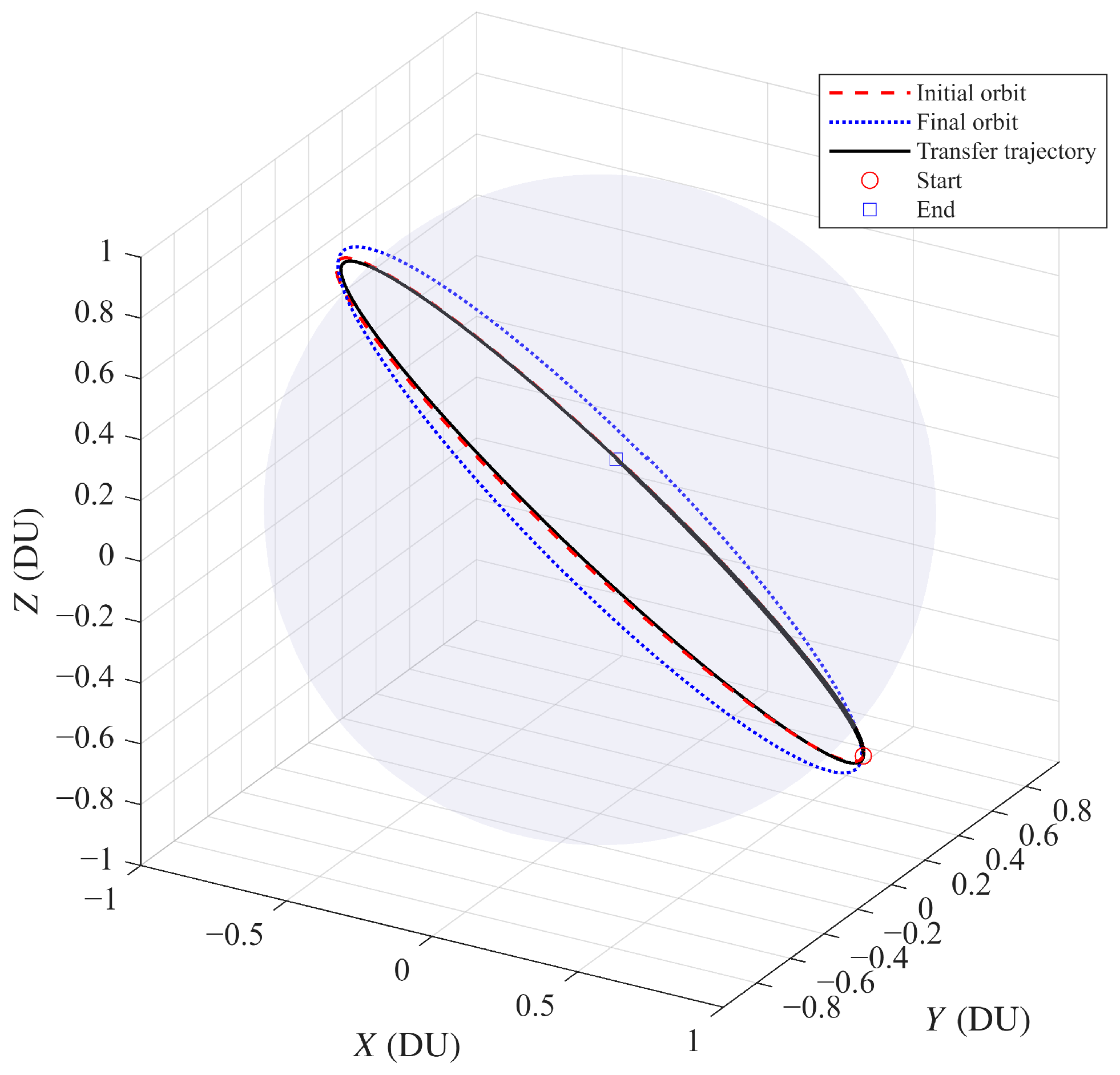
The result of the optimization is shown in Figure 1. The spacecraft successfully transfers from the initial orbit to the target orbit.

The three-dimensional trajectory exhibits smooth, continuous motion, and the spacecraft completes approximately one full orbit before reaching the target position. This probably results from the limited thrust magnitude relative to the spacecraft mass. The trajectory smoothness validates the third-order accuracy of the Hermite–Simpson discretization, which ensures continuous position, velocity, and acceleration profiles.

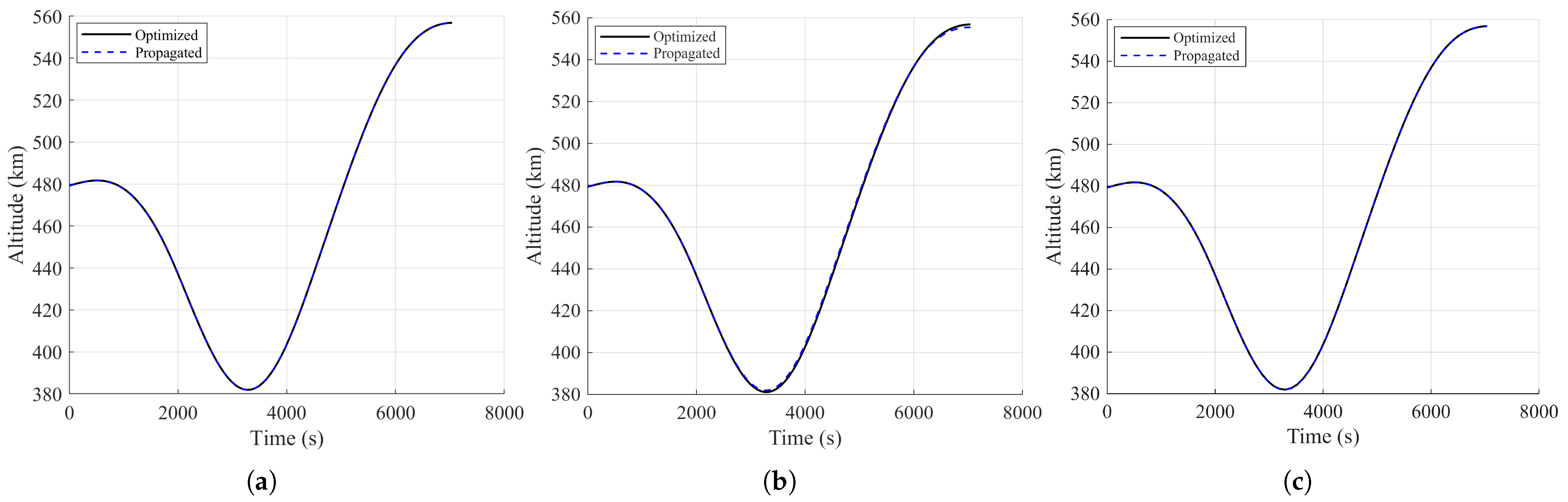
To verify the effectiveness and optimality of the method, the classical trapezoidal-based SCP (T-SCP) method and the pseudospectral-based SCP (P-SCP) method are compared. The orbital altitude curves for the three methods are shown in Figure 2.

The three methods exhibit different accuracy levels when compared against the reference numerical solution computed using a high-precision Runge-Kutta integrator. The orbital altitude profiles obtained by the Hermite–Simpson and pseudospectral methods closely match the reference solution throughout the entire transfer. This agreement validates that both higher-order methods accurately capture the true nonlinear dynamics, including J2 perturbation and atmospheric drag effects. In contrast, the trapezoidal method exhibits significant deviation from the reference trajectory. This discrepancy stems from the accumulation of second-order truncation errors over the long integration period, demonstrating the inadequacy of low-order discretization for high-fidelity trajectory optimization.

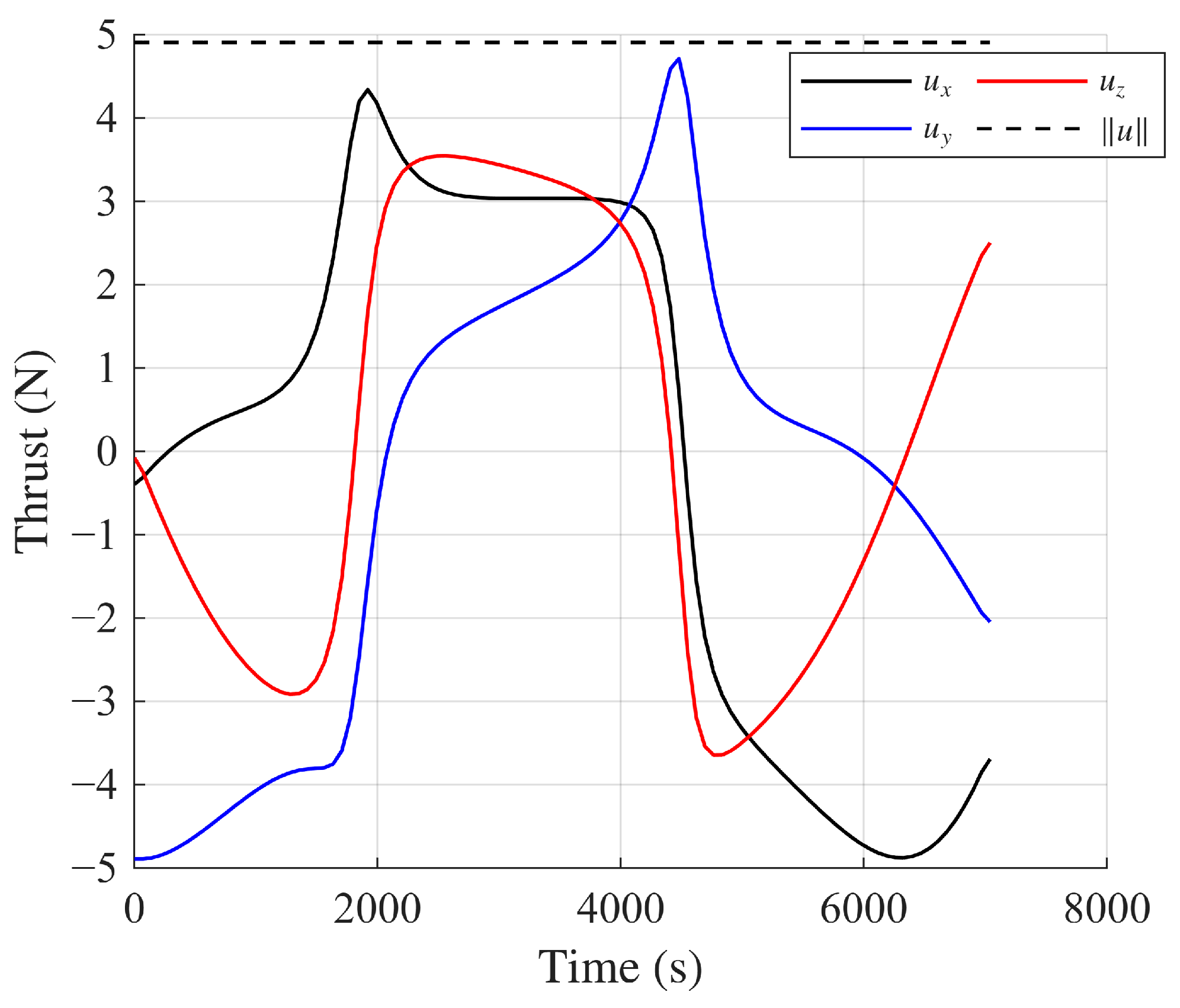
The thrust profiles are presented in Figure 3. The thrust magnitude remains within the allowable limit of 5 N throughout the transfer, satisfying the control constraint at all discretization nodes, while the direction varies continuously throughout the transfer to achieve the combined objectives of orbit raising, phase adjustment, and RAAN correction. Notably, the thrust magnitude remains consistently at or near the maximum allowable value for the majority of the transfer duration, exhibiting the characteristic bang-bang structure expected for time-optimal solutions.

Considering different numbers of discretization nodes, a quantitative comparison of the accuracy convergence rate and computational efficiency of the three methods is presented in the following tables. The results of the three methods are in

Table 4. Position and velocity errors for single spacecraft scenario.

Nodes	T-SCP	HS-SCP	P-SCP
50	98101 m, 111.4 m/s	284.7 m, 0.33 m/s	6441.8 m, 6.60 m/s
100	23770 m, 26.97 m/s	17.80 m, 0.02 m/s	261.6 m, 0.26 m/s
500	935.0 m, 1.06 m/s	0.31 m, $4.4\times {10}^{-4}$ m/s	0.24 m, $2.3\times {10}^{-4}$ m/s
1000	233.0 m, 0.26 m/s	0.15 m, $2.0\times {10}^{-4}$ m/s	0.15 m, $1.6\times {10}^{-4}$ m/s

,

Table 5. Computation time for single spacecraft scenario (seconds).

Nodes	T-SCP	HS-SCP	P-SCP
50	10.45	10.90	11.79
100	12.32	13.24	13.22
500	72.58	68.71	77.36
1000	141.11	159.96	193.96

and

Table 6. Minimum transfer time (seconds).

Nodes	T-SCP	HS-SCP	P-SCP
50	7052.7	7039.7	7046.8
100	7042.7	7039.5	7041.3
500	7039.5	7039.4	7041.3
1000	7039.5	7039.4	7041.3

.

Table 4 presents the terminal position and velocity errors for the three discretization methods with varying numbers of nodes. All three methods demonstrate clear convergence as the number of discretization nodes increases but with different error magnitudes. The trapezoidal method, being a second-order accurate scheme, exhibits the largest errors across all node counts. This behavior is consistent with the theoretical expectation that the global error of the trapezoidal rule scales as $O(\Delta {\tau }^2)$. The pseudospectral method exhibits initially poor performance at low node counts followed by exceptional accuracy at high node counts, a characteristic behavior reflecting its spectral convergence properties. The initially large errors at 50 nodes indicate that the global polynomial basis functions have insufficient degrees of freedom to represent the trajectory features accurately. However, once the critical solution components are resolved, the error plummets rapidly due to the exponential convergence rate. This behavior makes pseudospectral methods particularly attractive for problems requiring very high accuracy, but less suitable when computational resources limit the number of nodes.

In contrast, the Hermite–Simpson method demonstrates substantially superior accuracy even with a limited number of nodes due to its third-order convergence property compared to the trapezoidal method. With a global error scaling of $O(\Delta {\tau }^3)$, this method achieves position errors of only 284.7 m even with 50 nodes and converges to 0.15 m with 1000 nodes, which confirms the high convergence efficiency of the method.

Velocity errors follow the same convergence pattern as position errors: the Hermite–Simpson method has outstanding advantages when nodes are fewer than 100.

The computation time increases with the number of discretization points, remaining on the same order of magnitude for all three methods. Although the Hermite–Simpson method has higher per-iteration computational complexity than the trapezoidal method due to the additional midpoint evaluations, the increase in total computation time is modest.

A critical observation emerges when considering the accuracy-to-cost ratio: when the number of discretization points increases from 50 to 100, the computation time for all three methods increases modestly (approximately 20%), while the accuracy of position and velocity predictions improves dramatically. This favorable scaling indicates that investing in additional nodes yields substantial accuracy improvements with relatively small computational overhead. In practical scenarios where both computational cost and accuracy must be balanced, the Hermite–Simpson method offers a clear advantage, delivering superior accuracy with only marginal increases in computation time compared to the trapezoidal method.

The transfer time results in Table 6 prove that increasing the number of discretization points improves solution optimality up to a threshold, beyond which further increases yield diminishing returns. For the trapezoidal and Hermite–Simpson methods, convergence is achieved at 100 nodes, with no improvement observed when increasing to 500 or 1000 nodes. This indicates that discretization error is no longer the limiting factor for optimality; instead, the convergence tolerance of the sequential convex optimization algorithm becomes the dominant factor. At the same number of discretization points, the Hermite–Simpson method consistently achieves the shortest transfer times. At 50 nodes, the Hermite–Simpson method achieves 7039.7 s, compared to 7052.7 s for T-SCP, with a 13 s (0.18%) improvement. The pseudospectral method fails to obtain the optimal time.

The comprehensive comparison across all metrics reveals that the choice of discretization method involves fundamental trade-offs between accuracy, computational cost, and solution optimality. The trapezoidal method, despite its simplicity and predictable scaling, requires significantly more nodes (5–10 times) to achieve the accuracy levels attainable by higher-order methods. This makes it suitable primarily for preliminary analysis where quick estimates are more valuable than precision, or for problems with very simple dynamics where high accuracy is unnecessary. The pseudospectral method has high accuracy, but requires the longest computation time. The Hermite–Simpson method emerges as the most balanced choice for general-purpose trajectory optimization. Its third-order accuracy provides substantial improvements over trapezoidal discretization while requiring about the same computation time as the trapezoidal method, making it practical for real-time or near-real-time applications such as onboard trajectory replanning. The consistency of its performance across different node counts and accuracy requirements makes it a reliable default choice for a wide range of mission scenarios.

4.2. Scenario 2: Multi-Spacecraft Constellation Aggregation

The second scenario extends the validation to a multi-spacecraft constellation aggregation mission, demonstrating the scalability and collision avoidance capabilities of the proposed method. This scenario involves ten spacecraft performing coordinated orbit transfers from an initial constellation configuration to a target formation while maintaining safe separation throughout the maneuver.

Table 7. Multi-spacecraft cluster scenario parameters.

Parameter	Value	Unit
Minimum safe distance ($d_{safe}$)	100	m
Safety factor ($\alpha$)	1.5	–
Number of nodes (N)	100	–
Maximum iterations	15	–
Trust region radius (initial)	0.5	–
Slack penalty weight ($\lambda$)	${10}^6$	–

presents the simulation parameters for the multi-spacecraft cluster scenario. The scenario involves ten spacecraft performing coordinated orbit transfers from an initial constellation configuration to a target line formation, with collision avoidance as a critical constraint.

The initial configuration distributes the ten spacecraft randomly within a constellation, with RAAN, argument of perigee, and true anomaly sampled from uniform distributions over their respective ranges. This random initialization creates diverse relative geometries that comprehensively test the collision avoidance mechanism under various encounter scenarios, including head-on approaches, overtaking maneuvers, and crossing trajectories. The target configuration requires each spacecraft to maintain its orbital plane while raising its orbit by 70 km and advancing its phase by 30°. This configuration ensures that spacecraft trajectories will intersect in three-dimensional space, necessitating active collision avoidance throughout the transfer.

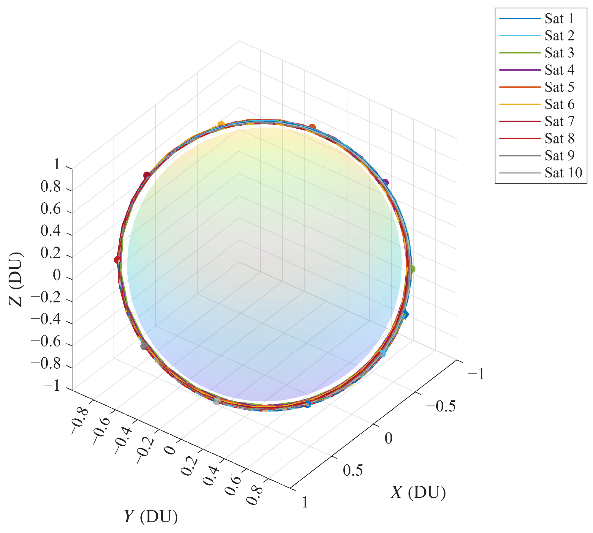
Figure 4 presents the three-dimensional trajectories of all ten spacecraft obtained using the Hermite–Simpson discretization method. The trajectories exhibit several notable characteristics that reflect the optimization objectives and constraints. All spacecraft follow smooth, continuous paths from their initial constellation positions to the target formation, with the trajectory curvature primarily determined by the gravitational field and the thrust direction optimization. The spatial distribution of the trajectories shows that spacecraft maintain adequate separation throughout the transfer, with no trajectory intersections or close approaches visible in the three-dimensional view.

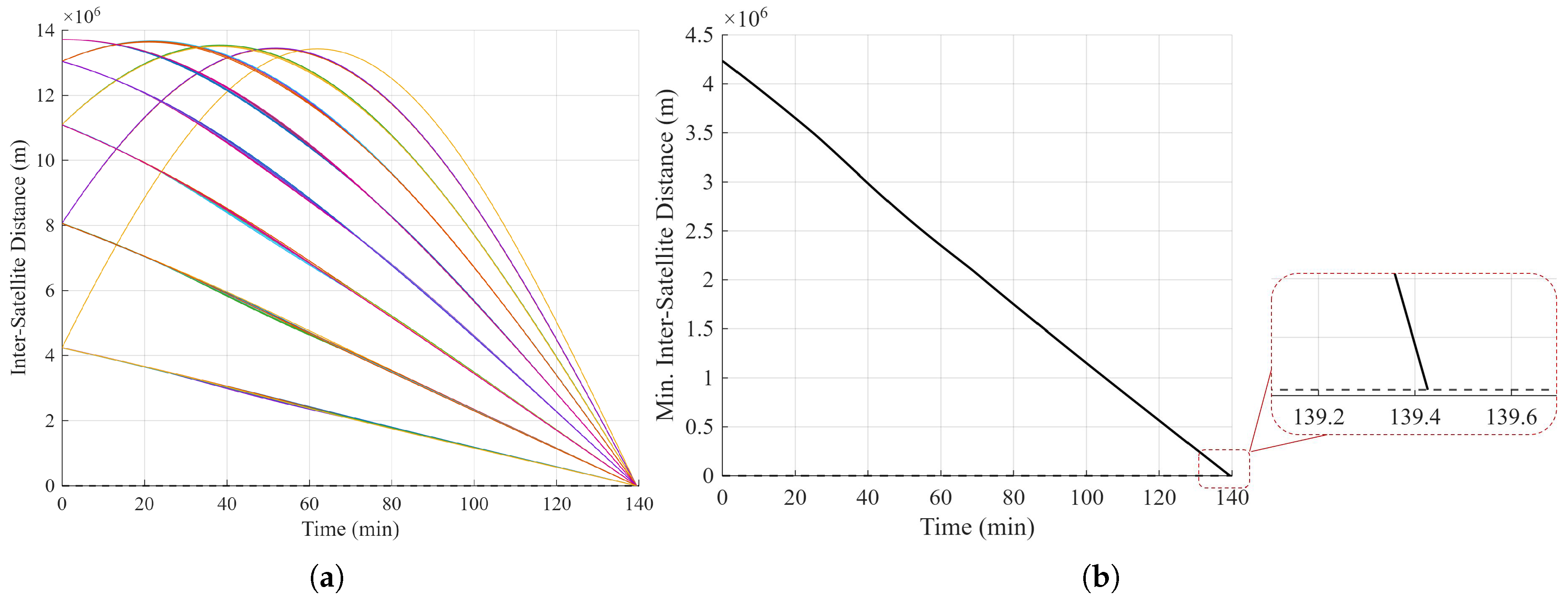
Figure 5 illustrates the minimum separation distances between all spacecraft pairs throughout the transfer. The results demonstrate that all spacecraft maintain separation distances well above the 100 m safety threshold, with the minimum observed distance being approximately 102.3 m. This margin above the safety threshold indicates that the collision avoidance constraints are active but not overly restrictive, allowing the optimizer to find efficient trajectories while maintaining safety.

The adaptive iterative collision warning mechanism effectively improves computational efficiency by triggering avoidance only for potential collision cases, rather than performing collision avoidance for all spacecraft. This significantly reduces the computational burden, especially for constellations with a large number of satellites that are widely dispersed.

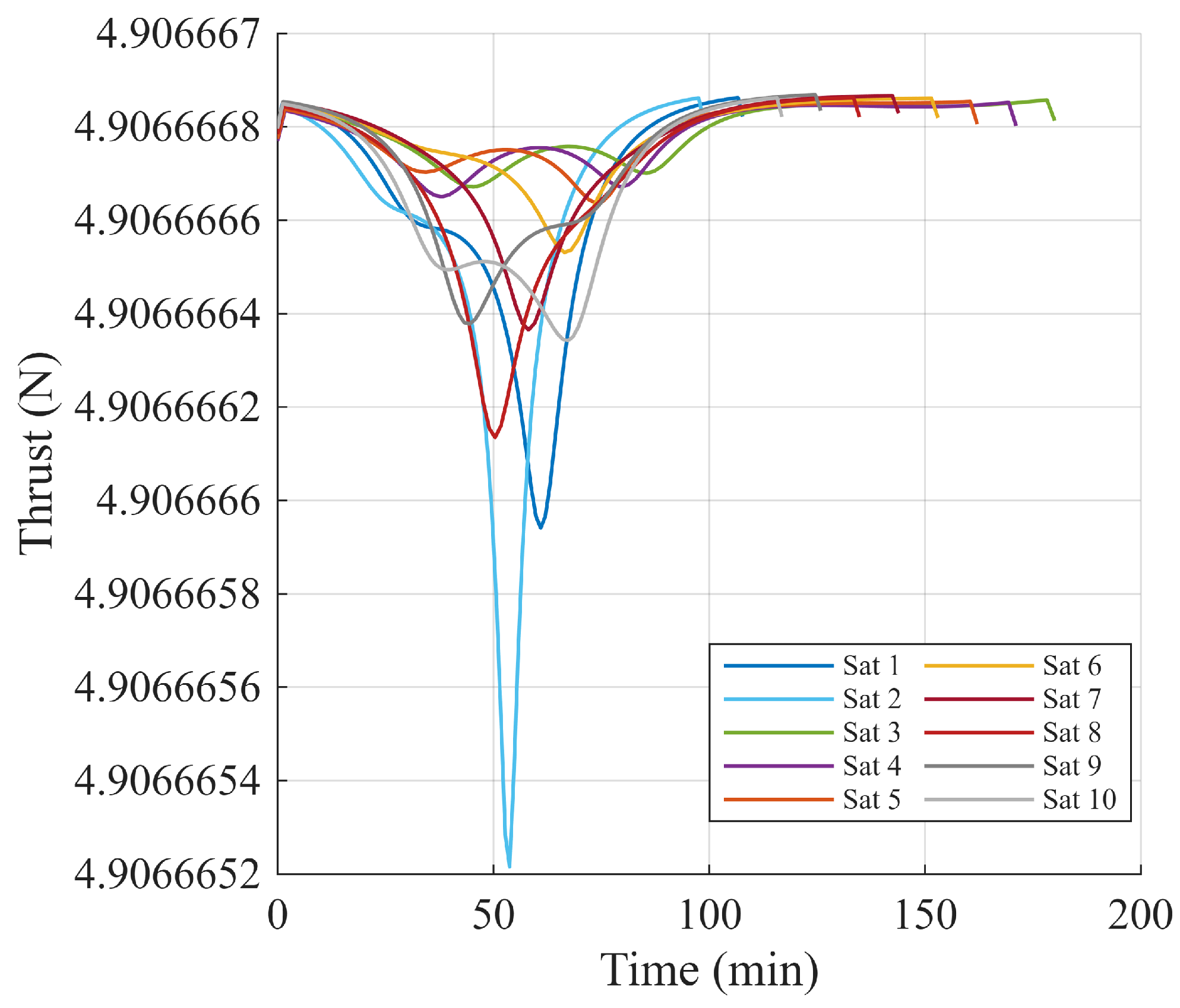
Figure 6 presents the thrust magnitude profiles for all ten spacecraft. The thrust profiles exhibit the characteristic bang-bang structure expected for time-optimal trajectories, with thrust magnitude at or near the maximum value for most of the transfer duration. The brief periods of reduced thrust correspond to collision avoidance maneuvers, where the optimizer reduces thrust in certain directions to maintain safe separation from other spacecraft. The consistency of thrust across spacecraft indicates that all spacecraft follow similar thrust profiles, differing only in the timing and small direction adjustments required for collision avoidance.

Table 8. Comparison of discretization methods for cluster scenario.

Metric	T-SCP	HS-SCP	P-SCP
Average transfer time (s)	8365.61	8363.42	8363.42
Computation time (s)	82.41	77.26	98.79
Max Position Error (m)	249,860.77	1.55	3751.11
Max Velocity Error (m/s)	277.3847	0.0387	4.0822

compares the performance of the three discretization methods for the multi-spacecraft cluster scenario.

The HS-SCP with adaptive iterative collision warning mechanism demonstrates advantages for the multi-spacecraft cluster scenario. This method improves computational efficiency by 6.2% compared with T-SCP and by 21% compared with P-SCP, which can be attributed to the combination of early warning collision avoidance and the adaptive trust region method. The collision warning mechanism reduces the computational load per iteration, while the adaptive trust-region update strategy and virtual control effectively avoid infeasibility and accelerate convergence.

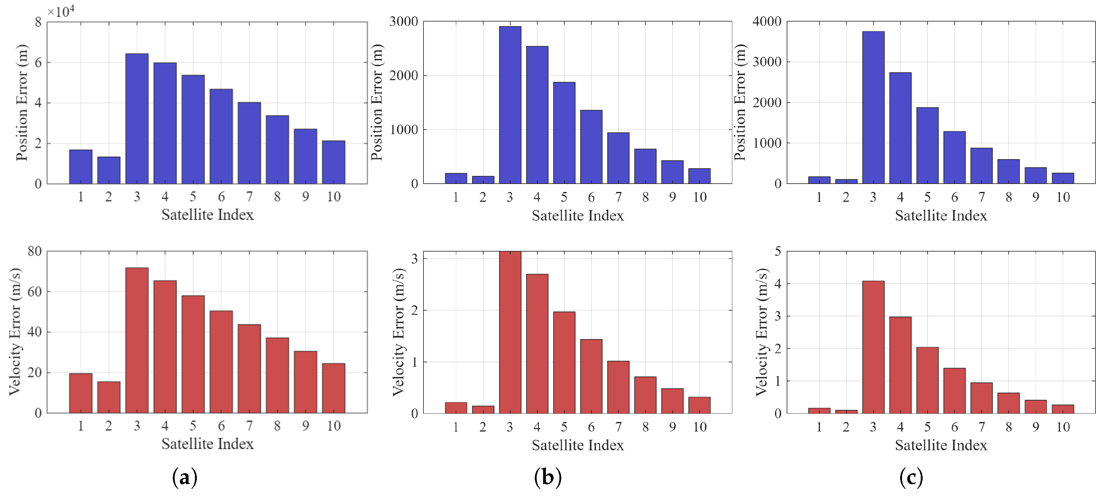
The transfer time results show that P-SCP and HS-SCP achieve the shortest transfer time in limited iterations, which is better than T-SCP. The following figure shows the comparison of position and velocity errors for the three methods, as presented in Figure 7.

The terminal position and velocity errors are critical metrics for evaluating the feasibility and practical applicability of trajectory optimization solutions. Large errors can lead to infeasibility issues that render the optimized trajectory unusable in real mission scenarios. The relationship between discretization accuracy and feasibility can be understood through the constraint satisfaction mechanism. The collocation constraints enforce dynamics consistency at discrete nodes, but the trajectory between nodes is only approximated. When discretization errors are large, the actual trajectory deviates significantly from the optimized trajectory, causing the terminal state to differ from the planned terminal state. This deviation is particularly problematic for multi-spacecraft scenarios where collision avoidance constraints must be satisfied throughout the entire trajectory, not just at discrete nodes. The simulation results demonstrate that the Hermite–Simpson method achieves terminal position errors below 10 m and velocity errors below 1 m/s, which are well within the feasibility requirements for practical missions. In contrast, the trapezoidal method with insufficient nodes produces position errors exceeding 10 km, which would render the solution infeasible for precision formation flying missions. Such large errors indicate that the trajectory cannot be reliably executed, and the spacecraft would miss its target position by a significant margin. The adaptive iterative collision warning mechanism further enhances feasibility by ensuring that collision constraints are satisfied throughout the trajectory. The velocity-dependent safety distance accounts for inter-node motion, preventing spacecraft from approaching each other between collocation points. This mechanism addresses the feasibility concern that arises from discrete trajectory representation, where collision avoidance at nodes does not guarantee collision avoidance between nodes.

4.3. Scenario 3: Monte Carlo Simulation

To validate the effectiveness of the algorithm, a total of 10,000 simulation scenarios were designed across four classical orbital configurations. The sequential convex optimization algorithm achieved 9100 successful runs with a success rate of 91%. The selected scenarios represent four typical orbital shells of the Starlink constellation, covering representative missions from low to high orbits and from narrow to wide inclination ranges. The parameters for each shell are shown in

Table 9. Starlink orbital shell configuration parameters.

Shell	Altitude (km)	Inclination (deg)	Altitude Range (km)	Inclination Range (deg)
Shell1	550	53.0	540–560	51–55
Shell4	540	53.2	530–550	51–55
D2C	360	53.16	340–380	51–55
High	1150	70.0	1110–1325	60–80

. The parameter settings for the SCP algorithm and the spacecraft are identical to those described previously.

Each shell employs Latin Hypercube Sampling (LHS) to generate $N_{\mathrm{shell}}=2500$ sets of random scenario parameters, containing 10-dimensional input variables:

$$\mathit{p}=[h_{\mathrm{init}},i_{\mathrm{init}},\Omega ,\omega ,\nu ,\Delta h,\Delta i,N_{\mathrm{planes}},N_{\mathrm{sats}/\mathrm{pl}},F_{\mathrm{phase}}]$$

(47)

where the altitude change $\Delta h\in [10,100]\mathrm{km}$ and inclination change $\Delta i\in [1°,5°]$. The first five parameters determine the basic shape of the orbit, the last three control the generation of the constellation, and the middle two restrict the generation range. With these control parameters, we ultimately randomly generate 10,000 orbital transfer missions under four scenarios.

The success rate statistics for each shell are shown in

Table 10. Success rate for each shell.

Shell	Total Scenarios	Successful	Failed	Success Rate
Shell1 (550 km)	2500	2500	0	100%
Shell4 (540 km)	2500	2500	0	100%
D2C (360 km)	2500	2500	0	100%
High (1110 km)	2500	1600	900	64%
Total	10,000	9100	900	91%

. Shell1, Shell4, and D2C shells all achieved 100% success rates, indicating that the SCP method has extremely high reliability in conventional orbital transfer missions. The High shell had a 64% success rate, with failed scenarios primarily concentrated in extreme cases with simultaneous large inclination changes ($\Delta i>4°$) and large altitude changes ($\Delta h>80\mathrm{km}$).

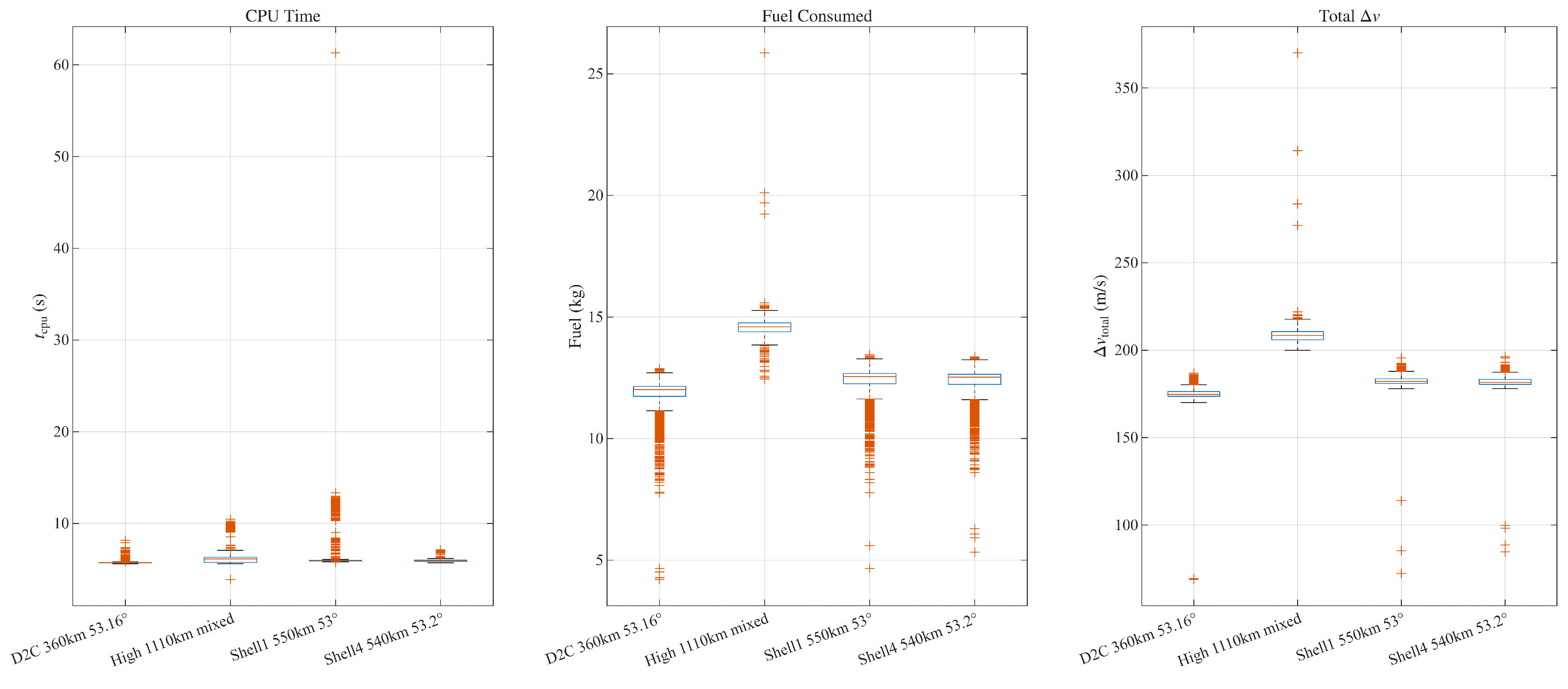
Box plots are adopted to visualize the central tendency, fluctuation range and outliers of key performance metrics across diverse working conditions, while bar charts are used to characterize the discrete distribution of success rates and error frequencies.

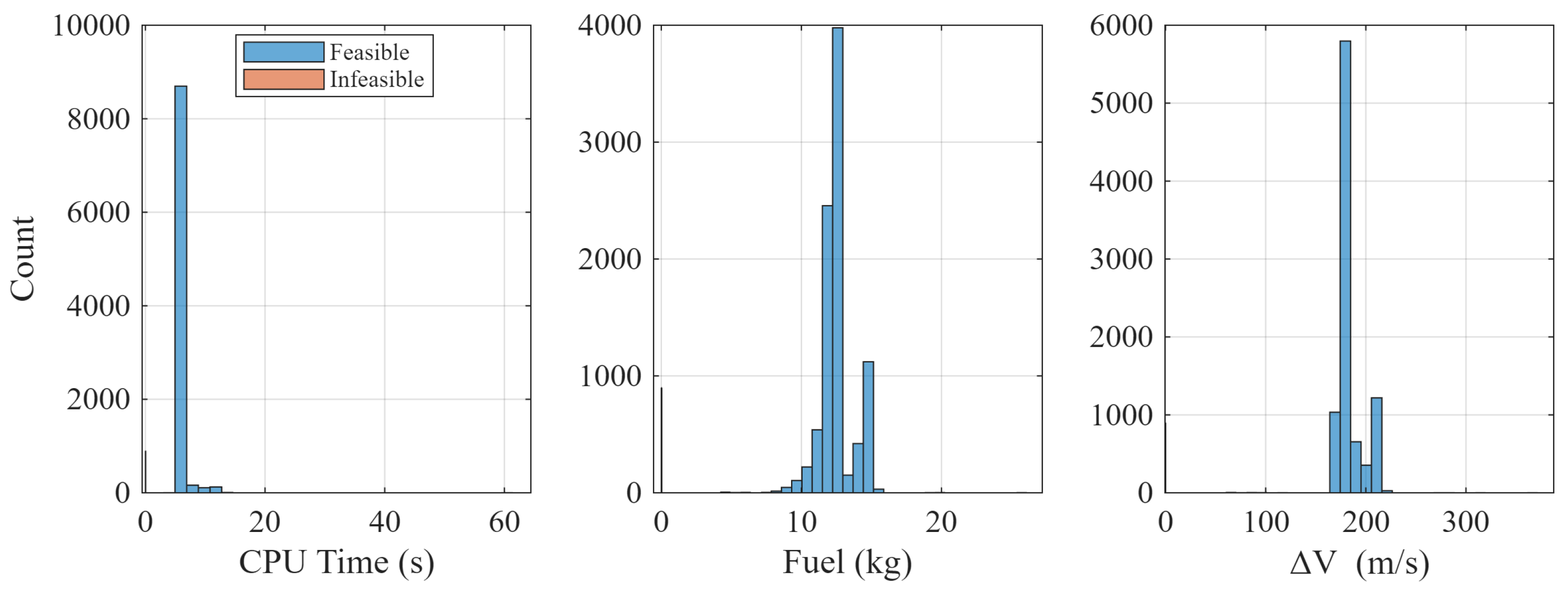
Figure 8 shows the histograms of computation time, fuel consumption, and velocity increment under successful scenarios. It can be observed that the computation time is relatively stable, mostly within 10 s, and the distributions of fuel consumption and velocity increment are also relatively concentrated. This is because, under the scenario settings, the changes in orbital transfer altitude and orbital plane are not particularly large. At the same time, it can be seen that these results are reasonably consistent with practical expectations, with no obvious outliers, indicating that the algorithm can converge to a reasonable solution in most cases.

Figure 9 shows the boxplot of computation time for successful scenarios in each shell. The median computation times for Shell1, Shell4, and D2C shells are all approximately 6 s, while the High shell is slightly higher. The D2C shell has the lowest fuel consumption with a median of approximately 12 kg due to its lower orbital altitude, higher velocity increment, and shorter orbital period. The High shell has the highest fuel consumption, with a median of approximately 15 kg, and the largest dispersion, which are related to its wide range of altitude and inclination changes. The optimization results for the 550 km and 540 km orbits are relatively close, indicating that when the orbital transfer conditions are similar, the fuel consumption for the transfer is also similar. The velocity impulse is also consistent with the fuel consumption.

5. Discussion

This paper proposes a high-precision adaptive sequential convex programming (SCP) method with a collision warning mechanism for spacecraft trajectory optimization involving long-distance transfers between adjacent orbital planes. The proposed method offers advantages in computational efficiency, accuracy, and robustness. First, an adaptive trust region strategy and slack variables are introduced. The trust region ensures the validity of linearization, while the slack variables provide a feasibility margin and are penalized in the objective function. This effectively prevents convergence failures caused by strong nonlinearities or large state variations over long distances, and it accelerates convergence. Additionally, the third-order accurate Hermite–Simpson method is employed instead of the commonly used trapezoidal rule, significantly reducing the accumulation of linearization errors over long transfer arcs and avoiding the resulting infeasibility of convex subproblems. In addition, a collision warning mechanism is incorporated: during the sequential iterations, collision avoidance constraints are computed only for spacecraft that have entered the warning zone. This reduces the computational burden while maintaining safety, greatly improving efficiency, and is particularly meaningful for constellation aggregation missions. Furthermore, the simulation scenarios include both in-plane orbit raising and transfers to adjacent orbital planes, demonstrating broad applicability and robustness. The method effectively resolves the infeasibility issue in non-coplanar transfers. Monte Carlo simulations across 10,000 random scenarios covering four Starlink orbital shells further confirm the method’s reliability, achieving a 91% overall success rate with a 100% success rate for LEO shells. In summary, the proposed method shows great potential for trajectory optimization in satellite clusters and constellation aggregation transfers.