Article

Adaptive Model Predictive Control and Safety Region Design for Multi-Body Satellite Separation

Space Engineering University, No. 1 Bayi Street, Huairou District, Beijing 101416, China
*
Author to whom correspondence should be addressed.
Aerospace 2026, 13(8), 672; https://doi.org/10.3390/aerospace13080672
Submission received: 2 December 2025 / Revised: 22 January 2026 / Accepted: 28 January 2026 / Published: 28 July 2026
(This article belongs to the Section Astronautics & Space Science)

Abstract

In order to ensure the safe separation and deployment of multi-body satellites, an adaptive model predictive control algorithm (AMPC) with an adaptive safety region is proposed in this study. First, the dynamic model of multi-body satellite separation is formulated to account for the momentum generated by sub-satellite separation on orbital altitude. Second, an adaptive safety region applicable to sub-satellite separation is designed through geometrical derivation based on the relative E/I vector framework. Finally, the safety region, which possesses clear geometric significance, is integrated into the AMPC framework to be solved as a set of control terminals and fitted by a neural network to reduce computational pressure. In conclusion, comparative simulations show that the proposed algorithm effectively reduces the variation in orbital altitude due to momentum by 78.4% and reduces the mission duration by 19.4%. This algorithm balances the momentum coupling effect and safety constraints during the separation of multi-body satellites and is suitable for unmanned, intelligent, and autonomous spacecraft control systems.

1. Introduction

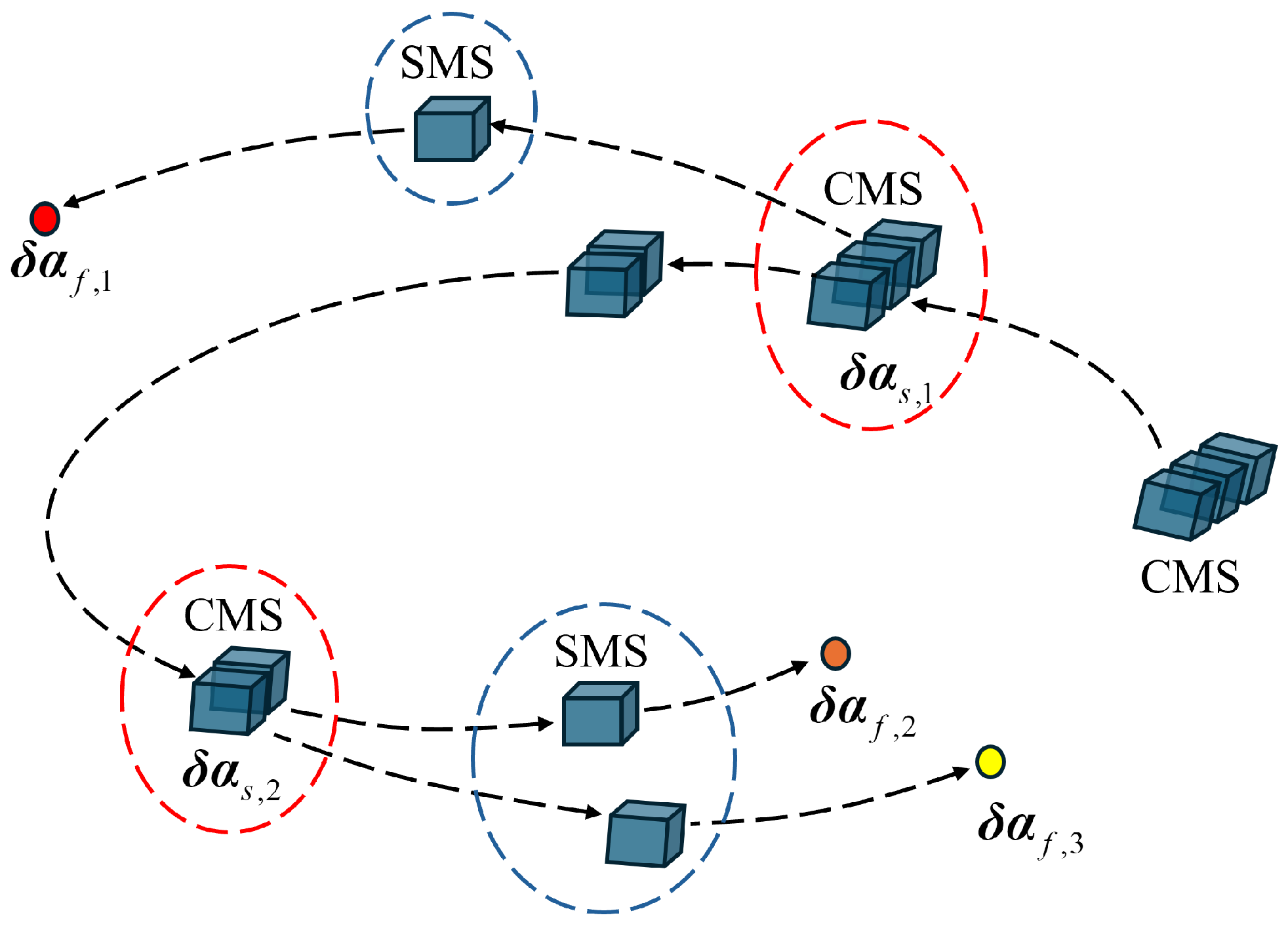
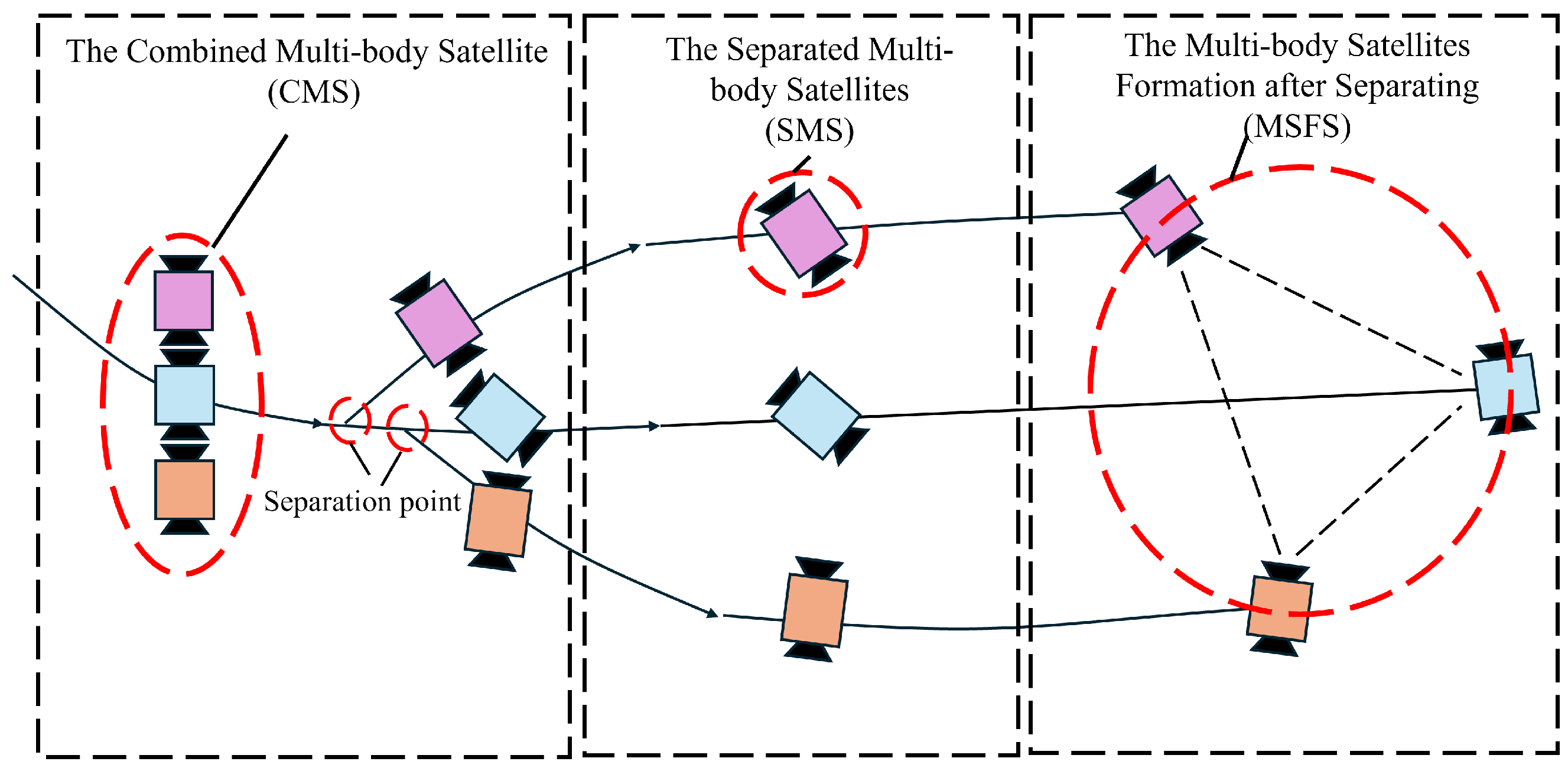
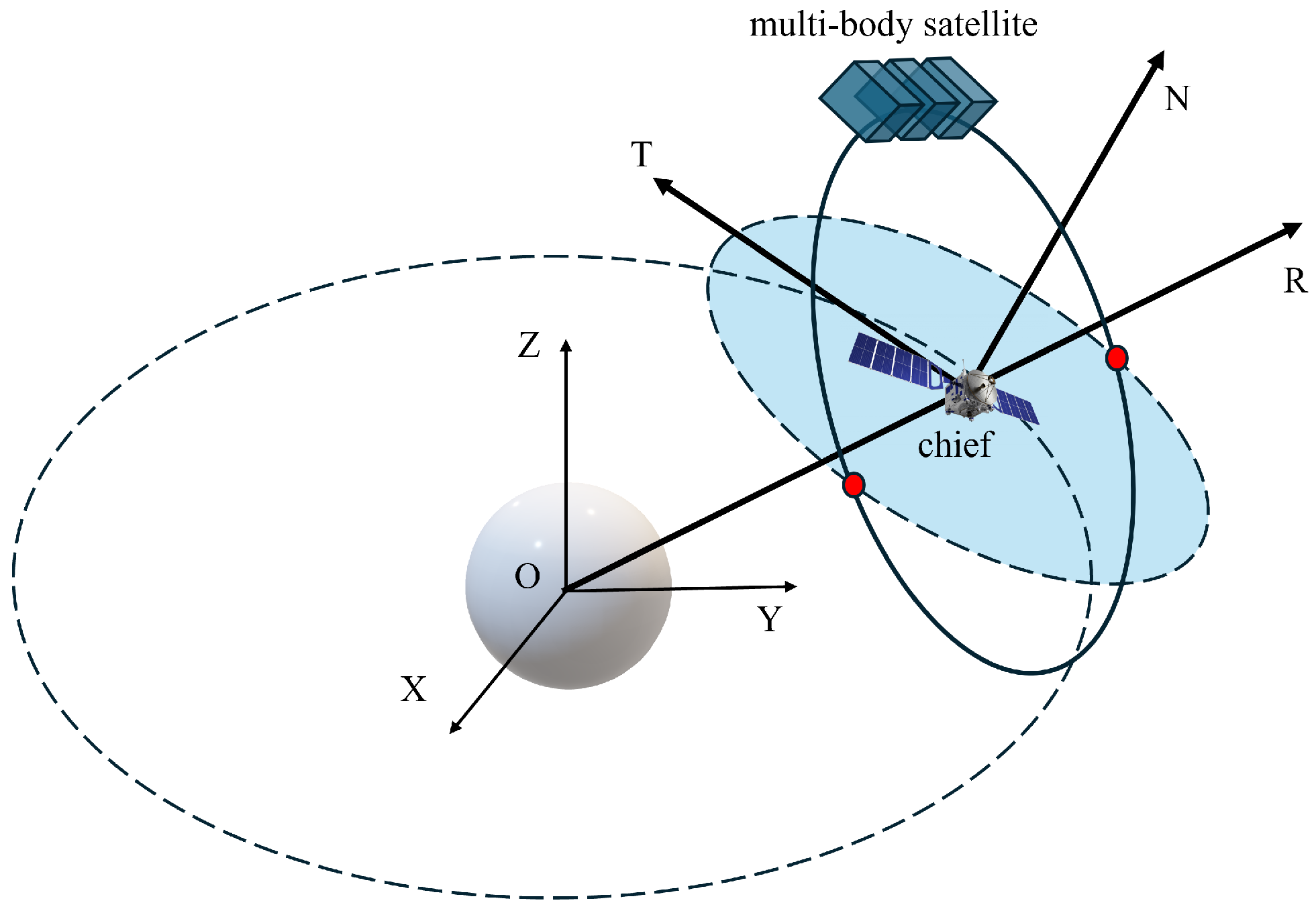
In recent years, scientists have developed the combined multi-body satellite (CMS), which consists of separate multi-body satellites (SMSs) of similar mass, structure, and volume, interconnected by compliant docking joints. It can be customized with diverse functions through reconfiguration transformations such as bending, twisting, and polymeric separation to meet specific mission requirements [1,2,3,4,5,6,7,8,9]. Among these, the CMS separation mission is similar to deploying a single spacecraft from a satellite dispenser or launch vehicle. Specifically, the SMS is delivered to a predetermined orbit via mechanical ejection, forming a safe, collision-free formation. The definition of the CMS is shown in Figure 1.
In the context of spacecraft formation, deployment, and reconfiguration, some studies have transformed numerical solution problems into nonlinear programming problems, which are then solved via intelligent optimization algorithms or control algorithms. Wang et al. [10] proposed self-organizing control rules for satellite cluster orbital reconfiguration based on artificial potential functions. These rules enable clusters to spontaneously reconfigure, distribute uniformly, and maintain safe distances. Minan et al. [11] addressed the deployment challenges of continuous-thrust tethered satellite systems by employing convex optimization techniques. In order to mitigate uncertain disturbances during collision-avoidance maneuvers in satellite clusters, Li et al. [12] developed velocity-obstacle-based terminal constraints and control laws using distributed model predictive control (DMPC).
In recent years, some studies have achieved large-scale satellite formation deployment via MPC algorithms. Pippia et al. [13] proposed a model predictive control (MPC) algorithm integrated with sequential convex programming for the reconfiguration of clusters comprising hundreds of spacecraft. Additionally, Menegatti et al. [14] created a collision-avoidance algorithm based on artificial potential functions for cooperative flight control in formations executing avoidance maneuvers using DMPC. Collectively, these studies show that optimal control methods, particularly MPC, effectively handle collision avoidance and thrust constraints in large-scale satellite cluster reconfiguration. Unlike the deployment missions in the aforementioned literature, due to the existence of the law of conservation of momentum, the on-orbit separating spacecraft will induce offset errors in the X-Y-Z directions of the main body. Fang et al. [15] noted that a launch vehicle’s orbital state changes abruptly upon satellite release due to momentum effects. However, SMSs often share similar mass and volume, and using mechanical mechanisms like catapults for separation affects the CMS’s momentum and orbital altitude significantly. Thus, further intuitive geometric analysis of CMS separation is required to ensure safe deployment.
Owing to its intuitive geometric interpretation, the relative E/I vector framework has been widely applied in related research, such as collision avoidance in proximity operations and the design of deployment strategies for on-orbit spacecraft separation. In terms of adopting the E/I vector separation principle to ensure collision avoidance in proximity operations, Gaias et al. [16], focusing on the formation flight test of two non-cooperative satellites, examined the safety criteria for formation collision avoidance based on the distribution of minimum vertical flight distances. Peters et al. [17] investigated the influence of changes in the eccentric reference orbit during the circular-to-elliptical orbit transition on collision-free safe rendezvous trajectories. Liu et al. [18] derived a sequence of low-collision-risk impulsive maneuvers based on E/I vector theory and reconfigured collision-free maneuvering paths for sub-satellites via comprehensive geometric analysis. The authors proposed a maneuvering method for the safe deployment of nanosatellites, which analyzes the safety distance constraints between the launch vehicle (LV) and the released satellite (RS), ensuring the safety of nanosatellite separation even without additional maneuvering. Regarding on-orbit formation separation deployment, Wang et al. [19] classified fuel-optimal satellite reconfiguration deployment scenarios into four categories and derived optimal and suboptimal control schemes. Roychowdhury et al. [20] adjusted the deployment vectors for the mission scenario in which two nanosatellites are deployed in a spiral orbit and proposed an improved deployment strategy to increase the chance of success for future deployment missions. Koenig et al. [21] considered sensor and actuator calibration operations, specifying the need for each sub-satellite to undergo a period of orbital drift after deployment, using nonlinear small-thrust control to eliminate errors.
Furthermore, setting safety constraints through geometric analysis within the E/I vector model not only enables spacecraft separation deployment but also ensures safe collision avoidance between individual spacecraft. In the work by D. et al. [22], a rectangular safety region was initially established based on the relative E/I vector model, which laid the foundation for the subsequent definition of safety constraints. Wang et al. [23] studied the analytical solution for spacecraft separation in orbit under general passive safety constraints and categorized reconfiguration deployments as either in-plane or out-of-plane. They proposed an innovative geometric solution that theoretically guarantees passive safety and verifies the optimality of the algorithm through simulation. The aforementioned literature used E/I vector analysis to define safety constraints and derived analytical solutions for impulsive maneuver deployment. This method works for the safe separation of a single on-orbit spacecraft. However, for multiple separations, vector dimensions and variable counts increase, and the dynamics become more complex. In such cases, separation strategies based on geometric intuition are ineffective in large-scale scenarios.
Therefore, to meet the mission requirements for the separation and deployment of sub-satellites from a multi-body satellite, it is necessary to propose a combined scheme of geometric separation constraint conditions for maintaining a safe distance and an optimization algorithm capable of solving large-dimensional variables. Based on the aforementioned literature, this work makes several innovative contributions:
  • Dynamics are modeled to analyze momentum-influenced multi-body satellite separation used the relative E/I vector framework. Geometric analysis derives safe separation constraints related to the argument of latitude and constructs an elliptical safe separation region design method.
  • A multi-body satellite separation algorithm is proposed, which defines the safe separation region as a terminal constraint and integrates MPC and ADP. It effectively incorporates safety constraints with clear geometric meanings into the optimal control framework and solves numerical solutions via fitting, thereby reducing momentum-induced orbit altitude deviations and shortening overall mission completion times.
In Section 2.1, the basic knowledge and definition of the multi-body satellite separation mission are introduced. In Section 2, we analyze the separation mission, discuss the momentum-influenced relative orbital dynamics model, and define the safe region. In Section 2.5, a separation algorithm combining model predictive control and adaptive dynamic programming is designed. In Section 3, we perform comparative simulations to verify the model. In Section 4, we discuss the results. In Section 5, we summarize the entire article.

2. Materials and Methods

2.1. Relative Motion Model

The reference satellite is defined as the origin of the LVLH coordinate system, and the trajectory of the CMS relative to it is shown by the black solid elliptical trajectory in Figure 2. The relative motion of the CMS with respect to the reference satellite can be described using dimensionless relative orbital elements (ROEs) [18]:
δ α = δ a / a c δ λ δ e x δ e y δ i x δ i y = ( a d a c ) / a c u d u c + ( Ω d Ω c ) cos i c e d cos ω d e c cos ω c e d sin ω d e c sin ω c i d i c ( Ω d Ω c ) sin i c
where c and d represent the reference satellite and the maneuvering satellite, respectively, and  u = M + ω represents the mean argument of latitude. δ a represents the relative semi-major axis, δ λ represents the relative mean argument of latitude, δ e = δ e x δ e y T represents the relative eccentricity vector, and the relative inclination vector is denoted by δ i = δ i x δ i y T . The impulse vector in this coordinate system is defined as Δ v = [ Δ v R , Δ v T , Δ v N ] T . In near-circular orbits, the semi-major axis is defined as a, and the mean angular velocity as n, and the impulsive velocity change in the aforementioned RTN coordinate system can be expressed as follows:
Δ δ α = B ( u ) Δ v B ( u ) = 1 n a 0 2 0 2 0 0 sin u 2 cos u 0 cos u 2 sin u 0 0 0 cos u 0 0 sin u
The ROE state transition equation achieved by a single impulsive maneuver is
δ α ( u ) = Φ ( u , u 0 ) δ α ( u 0 ) + u 0 u Φ ( u , t ) Δ δ α ( t ) d t
Given the definition ψ ( u , u 0 ) = u 0 u Φ ( u , τ ) B ( τ ) d τ , within the integral interval u 0 , u , it can be further expressed as
δ α ( u ) = Φ ( u , u 0 ) δ α ( u 0 ) + ψ ( t , t 0 ) Δ v
To facilitate geometrically intuitive analysis of multi-body satellite separation, the polar coordinates of the relevant E/I vectors are introduced [19,23,24]:
δ e δ i = δ e x δ e y δ i x δ i y = δ e cos φ δ e sin φ δ i cos θ δ i sin θ
where φ and θ are the argument of latitude and the longitude of the ascending node of the relative orbit, respectively. The system in which the relative eccentricity vector is usually displayed in δ e x , δ e y and δ i x , δ i y coordinates is the (inertial) perifocal reference system. The relative position vector between the reference satellite and the multi-body satellite in the RTN frame can be expressed as [18]
δ e R / a = δ a δ e cos ( u φ ) δ e T / a = δ λ 3 2 δ a u + 2 δ e sin ( u φ ) δ e N / a = δ i sin ( u φ )
The formation reconfiguration is defined as an ROE transfer from the initial state to the final state: δ α 0 to δ α f . The three-impulse fuel-optimal solution for formation reconfiguration is [23]
Δ v T = Δ v T 1 = η n a Δ δ e / 8 , u T 1 = β Δ v T 2 = η n a Δ δ e / 4 , u T 2 = β + π Δ v T 3 = η n a Δ δ e / 8 , u T 3 = β + 2 π
Δ v N = η n a δ i 1 δ i 0 , u N 1 = γ η n a δ i 2 δ i 1 , u N 1 = γ + π η n a δ i f δ i 2 , u N 1 = γ + 2 π
where Δ δ e = δ e f δ e 0 = Δ δ e , β = arctan Δ δ e y / Δ δ e x , γ = arctan Δ δ i y / Δ δ i x , γ , β 0 , π , η = sgn Δ δ e x cos β + Δ δ e y sin β , Δ v T , i , u i , and Δ v N , u N , i , i = 1 , 2 , 3 , respectively, correspond to the magnitude and phase of the velocity increment for the maneuver.

2.2. Definition and Related Assumptions of the Multi-Body Satellite Separation Mission

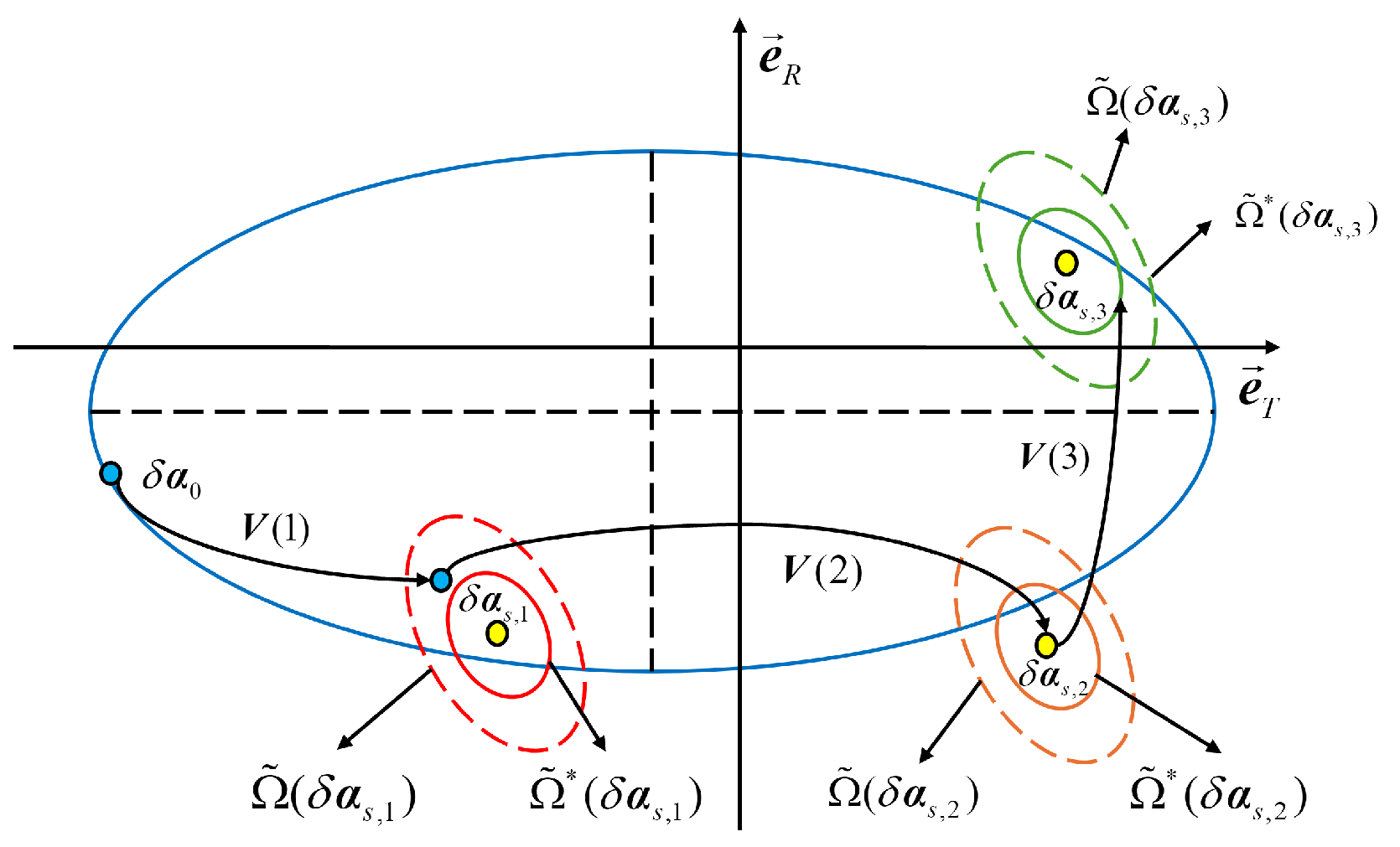
As shown in Figure 3, the SMS is equipped with autonomous maneuvering capability, and its target state is δ α f . Therefore, the mission of the CMS separating N SMSs is decomposed into N phases; in each phase, the CMS reaches the state set Ω ˜ ( δ α s ) suitable for the safe separation of the SMSs through impulsive maneuvers and performs the separation mission at a certain separation state δ α s within it. Subsequently, in the RTN coordinate system centered on the reference satellite, the mean argument of latitude u is taken as the key control parameter for ejection timing, and the geometric relationships under the E/I vector framework are analyzed to evaluate separation safety. The pertinent definitions and assumptions are articulated below.
The relative ROEs of the SMS with respect to the reference satellite are defined as
F = δ α f , 1 δ α f , 2 δ α f , N R 6 × n
Under the relative E/I vector framework, as the SMS separates from the CMS due to the momentum theorem, it causes a deviation in the semi-major axis of the CMS, denoted as Δ a . Thus, the cumulative error from a sequence of separations can be expressed as
D = Δ a 1 Δ a 2 Δ a N R 6 × n
The target state and separation state set for each SMS are defined as follows:
S = δ α s , 1 δ α s , 2 δ α s , N R 6 × n
Ω = Ω ˜ ( δ α s , 1 ) Ω ˜ ( δ α s , 2 ) Ω ˜ ( δ α s , N )
The maneuver sequence of the CMS and the mean argument of latitude u are defined as
V n = Δ v 1 Δ v 2 Δ v N R 3 × n
u = u 1 u 2 u N R 1 × n
The separation mission of the CMS is described as follows: Given the target states of the SMS as F and the maneuvering Equations (7) and (8) of the CMS, considering the orbital drift error D caused by separation, solve for the target states at each stage S , the terminal set Ω , and the velocity impulses V .
Assumption A1.
To simplify the problem, this paper does not consider the influence of impulsive maneuvers on the attitude of the multi-body satellite, but only considers the influence of impulsive maneuvers during separation on the orbit. Additionally, the velocity impulse generated during separation always satisfies 0 Δ v d e l Δ v s p r i n g .
Assumption A2.
Although out-of-plane maneuvers can change the orbital plane and improve separation safety, in the actual flight of spacecraft, impulsive maneuvers for changing the orbital plane consume substantial fuel, which will exert a significant impact on the entire optimization process. Therefore, this paper only considers in-plane separation maneuvers, including radial maneuvers and tangential maneuvers.

2.3. Momentum Analysis of Multi-Body Satellite Separation

Given the similarities of all SMSs in mass, volume, and structure, the separation mechanism applies impulsive maneuvers to the CMS based on the mass ratio. Thus, this section analyzes the impact of separation forces in different directions on the ROEs using the law of conservation of momentum [15,18].
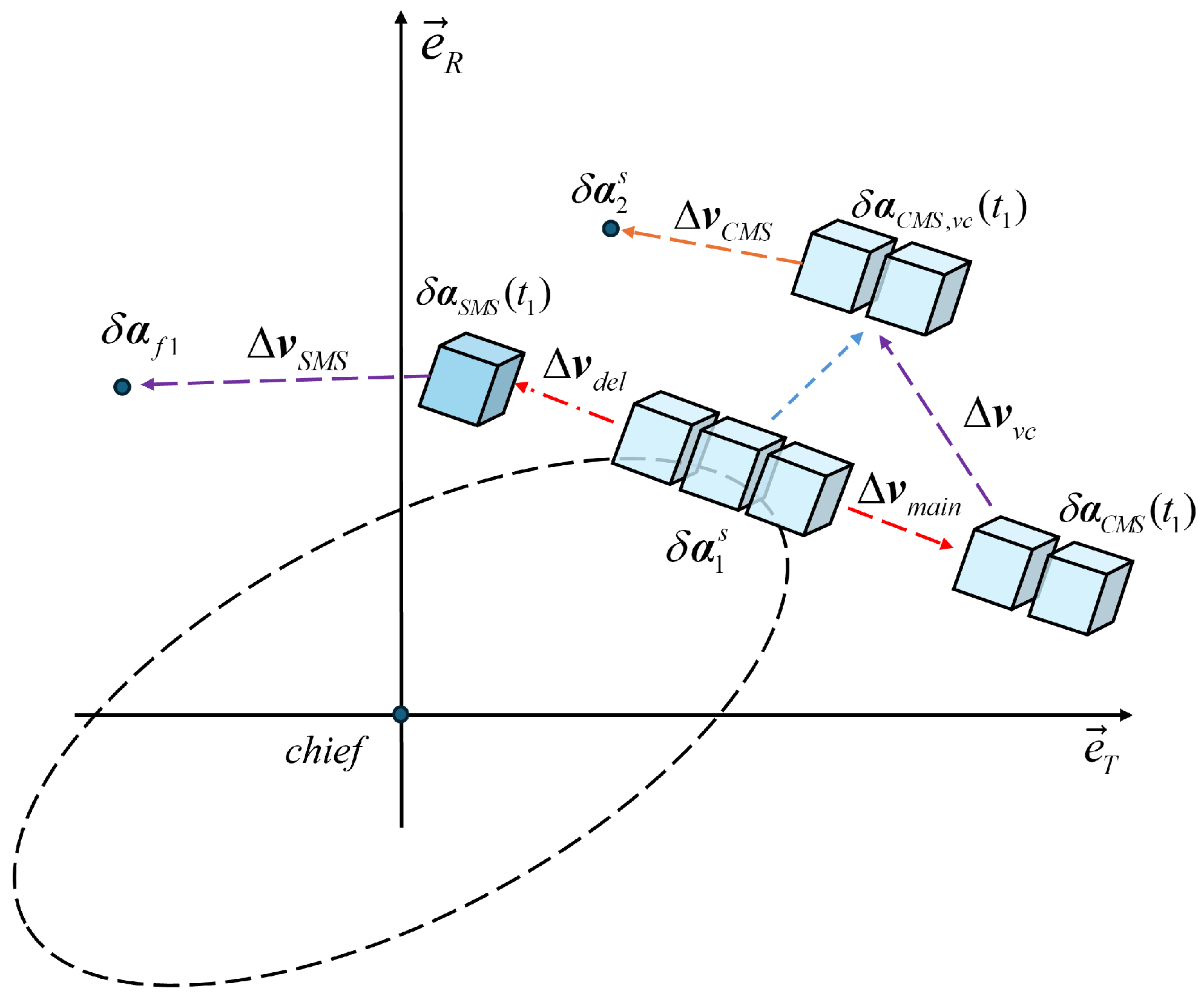
As illustrated in Figure 4, the system configuration is defined as follows: The SMS has a mass of m sep , while the CMS, which comprises N identical SMS units, has a total mass of M main = N m sep . Initially, both the SMS and CMS share a common state δ α ( u 0 ) , with the SMS designated to reach a target state δ α f . When the CMS is in state δ α s , 1 , momentum conservation dictates that the separation imparts the SMS with a relative velocity Δ v del , while the CMS acquires a velocity increment Δ v main . To mitigate the effects of this velocity change, the CMS executes a compensation maneuver Δ v vc , transitioning to the subsequent separation state δ α CMS , vc ( u 1 ) . Concurrently, the SMS employs its own propulsion capability through a maneuver Δ v SMS to achieve its designated target state δ α f 1 .
The SMS state variation over u 0 , u 1 can be expressed as
δ α SMS ( u 1 ) = Φ ( u 1 , u 0 ) δ α ( u 0 ) + ψ ( u 1 , u 0 ) Δ v del
Considering the momentum conservation before and after an SMS separation,
M v all = m sep v 1 + M main v main
where v a l l denotes the initial velocity of the entire satellite system, v 1 = v all + Δ v del denotes the velocity of the SMS, and the velocity of the CMS after separation is v main = v all Δ v main .
Define k = 1 ( N 1 ) .
The velocity variation is as follows:
Δ v main = Δ v del ( N 1 ) = k Δ v del
Incorporating (3), the error analysis of the ROEs is
Δ δ α = ψ ( u 0 , u 1 ) Δ v main = k Δ v del
The dynamical model of the CMS can be expressed as
δ α C M S ( u 1 ) = Φ ( u 0 , u 1 ) δ α ( u 0 ) + ψ ( u 0 , u 1 ) Δ v vc + ω k k Δ v d e l
where w denotes the separation flag ( ω k = 1 for a separated SMS, ω k = 0 for an unseparated SMS). The compensation impulse maneuver of the CMS is Δ v v c . Tangential or radial separation induces coupling effects on the relative orbital elements, making it difficult to intuitively determine which minimizes impacts. Thus, numerical simulations are used to compare these coupling effects. The ROEs of the chaser satellite are set as a δ α = 700 0 606.2 350 350 606.2 .
δ λ ( t ) = δ λ 0 3 2 δ a u t u 0
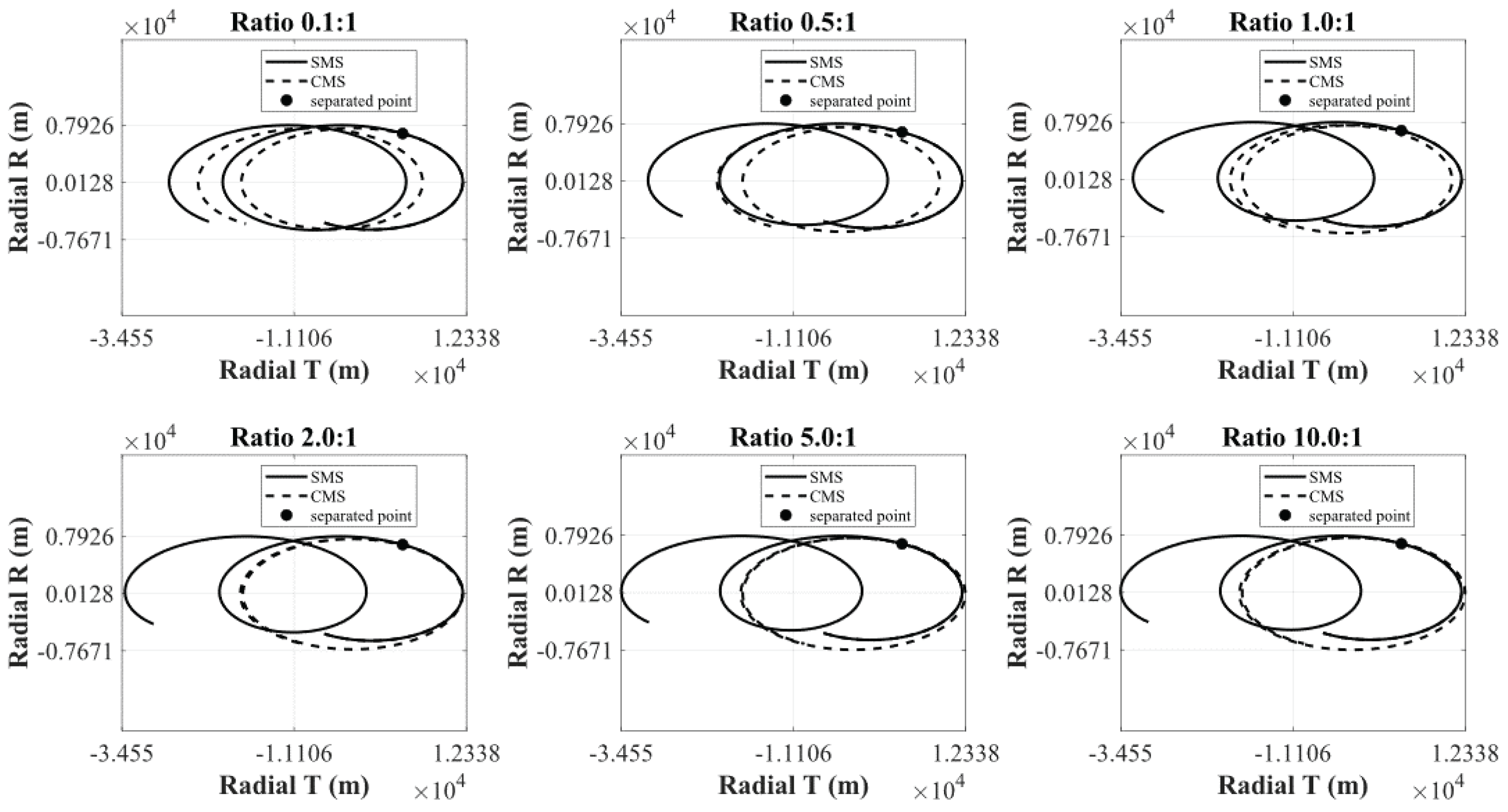
where δ λ 0 is the initial mean argument of the relative latitude, δ λ ( t ) is the mean argument of the relative latitude at the current time, u 0 is the initial mean argument of latitude, and  u t is the mean argument of latitude at the current time. Figure 5 shows diagrams of the trajectories of the tangential velocity component v t and the radial velocity component v r during the separation process under different v t / v r ratios. It can be observed that when the total maneuver velocity increment remains constant, the larger the v r component, the more significant the changes in the relative orbital configurations between the CMS and the SMS after separation, and the relative distance between the two modules exhibits periodic fluctuations. In contrast, with the increase in the v t component, due to the existence of orbital drift (20), the distance between the two separated modules is rapidly widened within two orbital periods.
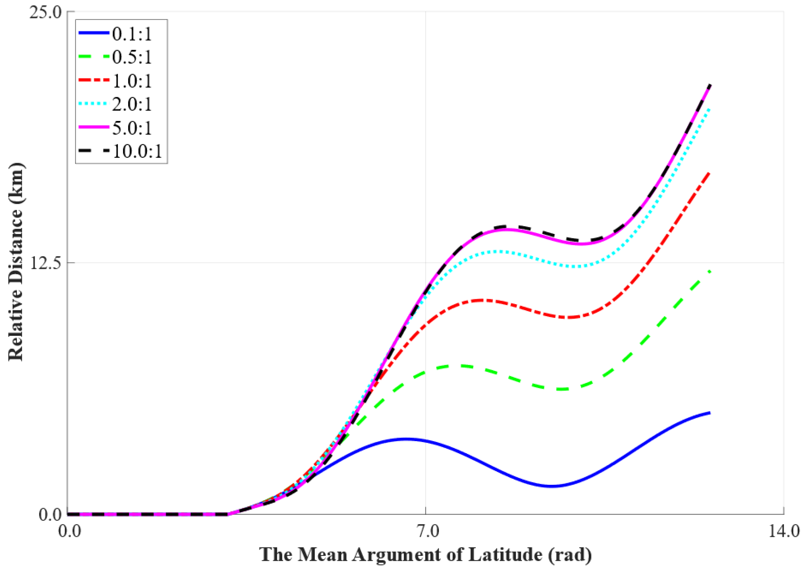
Furthermore, as shown in Figure 6, for  v t / v r ratios of 2.0:1, 5.0:1, and 10.0:1, the curves depicting the relative distance variation between the CMS and SMS (both before and after separation) exhibit a high degree of similarity. Therefore, if there are no specific requirements for the in-plane orbital configuration variation of the SMS during the separation process, given a fixed available velocity increment, adopting v t -dominated separation is more conducive to ensuring collision safety after satellite separation.
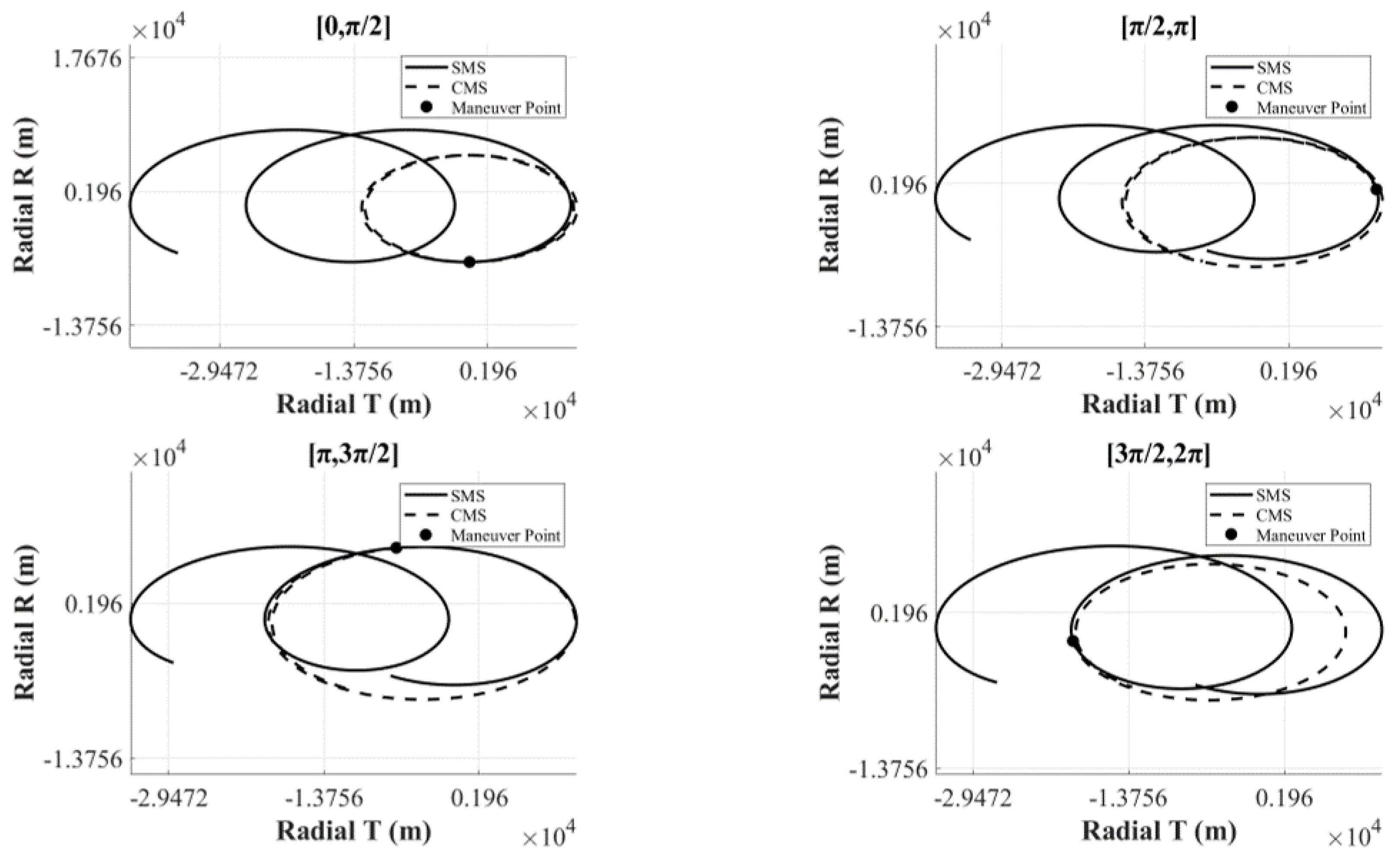
As shown in Figure 7, when separation is performed within the argument of latitude intervals [ π , 3 π / 2 ] and [ 3 π / 2 , 2 π ] , the post-separation trajectories of the CMS and the SMS overlap within one orbital period. By contrast, conducting separation in the argument of latitude intervals [ 0 , π / 2 ] and [ π / 2 , 3 π / 2 ] facilitates an increase in their relative distance over a short period.
In summary, if there are no specific requirements for the orbital shape of the CMS, and only a separation method adopting + v t and satisfying the argument of latitude intervals [ 0 , π / 2 ] and [ π / 2 , 3 π / 2 ] is used, the SMS and the CMS will maintain a safe relative distance through drift.

2.4. Safety Constraints for Successive Separation

The previous section derived a single separation mode applicable to the CMS. However, in practical engineering, the CMS consists of multiple SMSs. A rapid separation would introduce collision risks, while an overly slow separation would fail to complete the separation task in a timely manner. Therefore, this section focuses safety of successive separations to ensure both separation safety and timely separation completion.
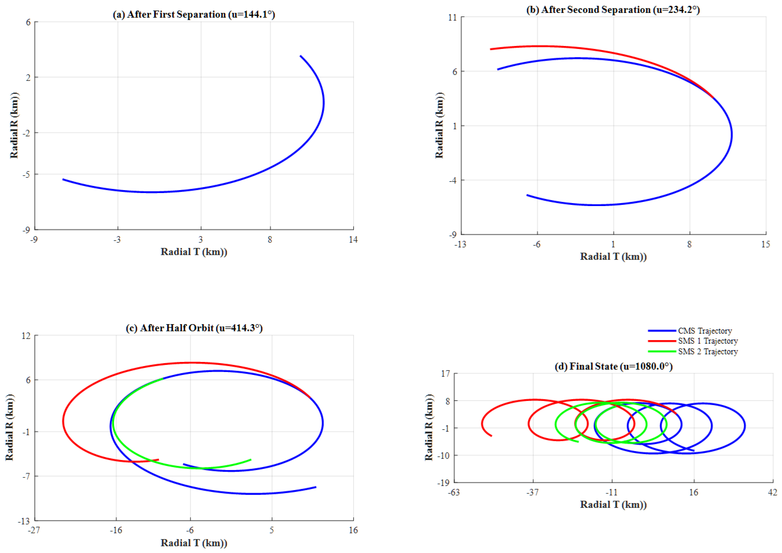
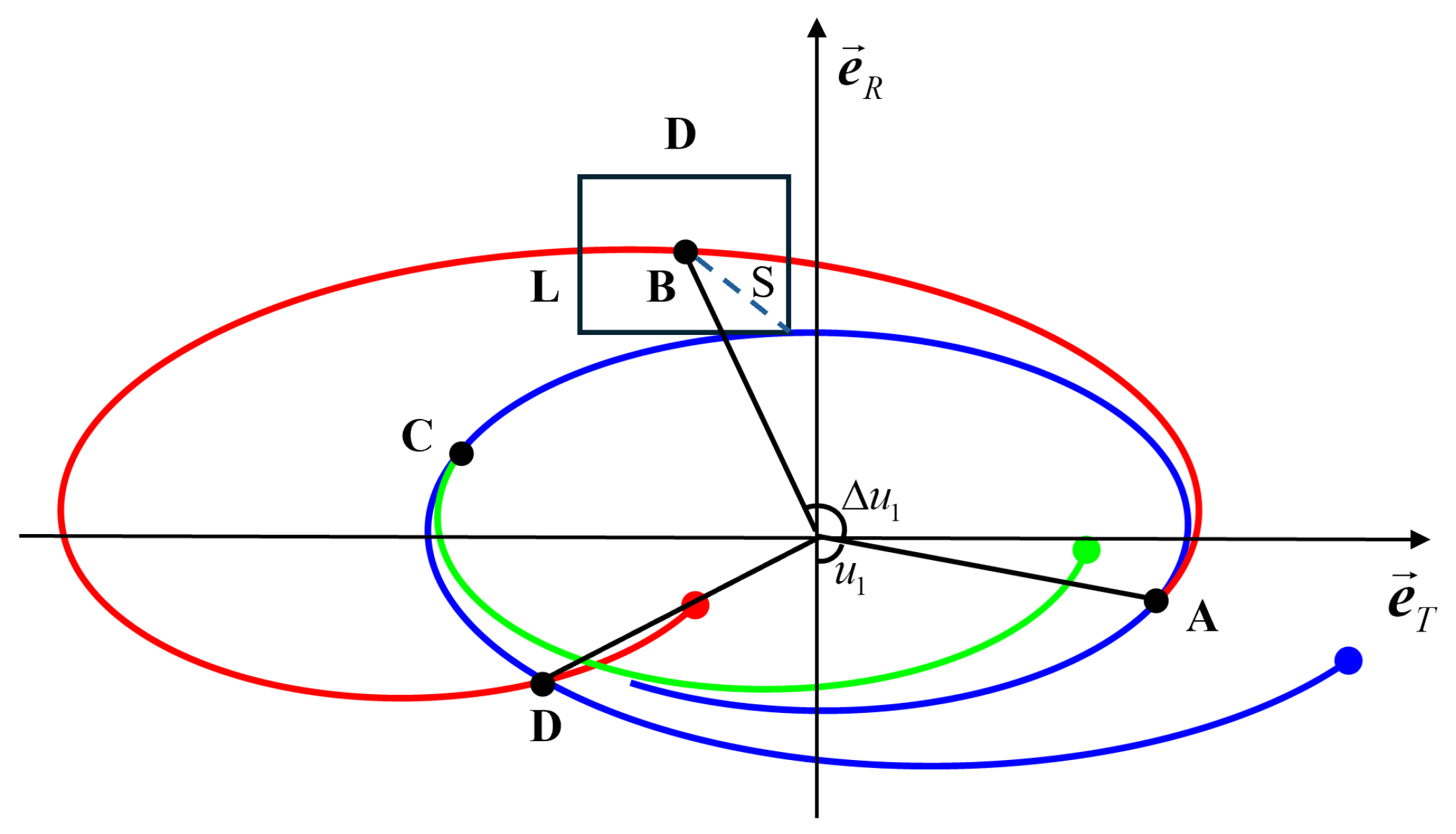
As illustrated in Figure 8, the first separation of the CMS is executed at the true anomaly u = 144 ° , with the subsequent separation occurring at u = 234 ° . After several orbital periods, the relative trajectories of SMS-1 with respect to both SMS-2 and the CMS display partial overlap, as shown in Figure 8c,d. When temporal factors are not taken into account, this scenario presents a potential collision risk. The mean argument of latitude of the first separation is defined as u 1 , and the generated drift magnitude is defined as Δ λ ( t ) . The interval between the current separation and the subsequent separation is defined as
u 2 = u 1 + Δ u
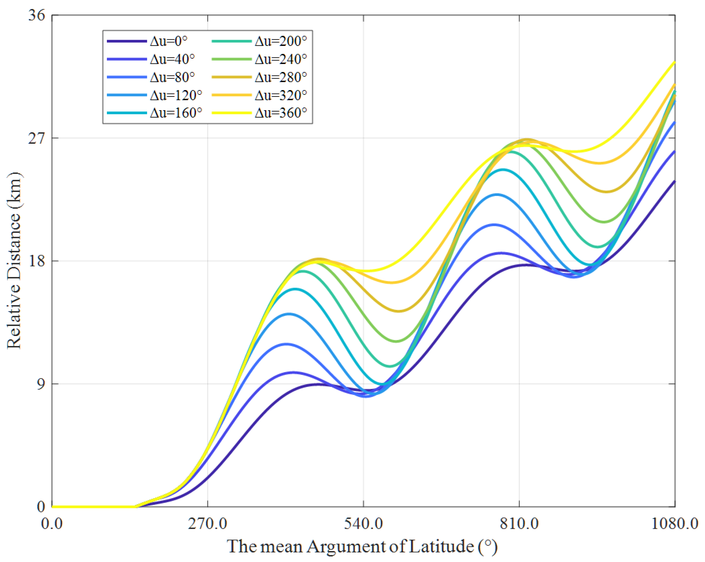
As shown in Figure 9, the relative distance between the two entities in the RTN coordinate system exhibits harmonic variation with the parameter Δ u , and the relative distance increases as Δ u increases. However, when Δ u exceeds 180°, the variation trend weakens. This indicates that the optimal value of Δ u is not simply the larger, the better, and that it is necessary to balance the setting of mission objectives.
The mean argument of latitude constraint for the next separation is defined as follows (with the derivation provided in Appendix A):
Δ u K 1 + Δ u λ , φ 2 + Δ u λ
where K 1 = D 2 + L 2 a · 9 4 δ a 1 2 3 δ a 1 δ e 1 + 4 δ e 1 2 , D denotes the tangential safety margin, and L denotes the radial safety margin. Δ u λ = ε · arctan Δ λ ( t ) Δ e , Δ e = e R 2 + e T 2 .
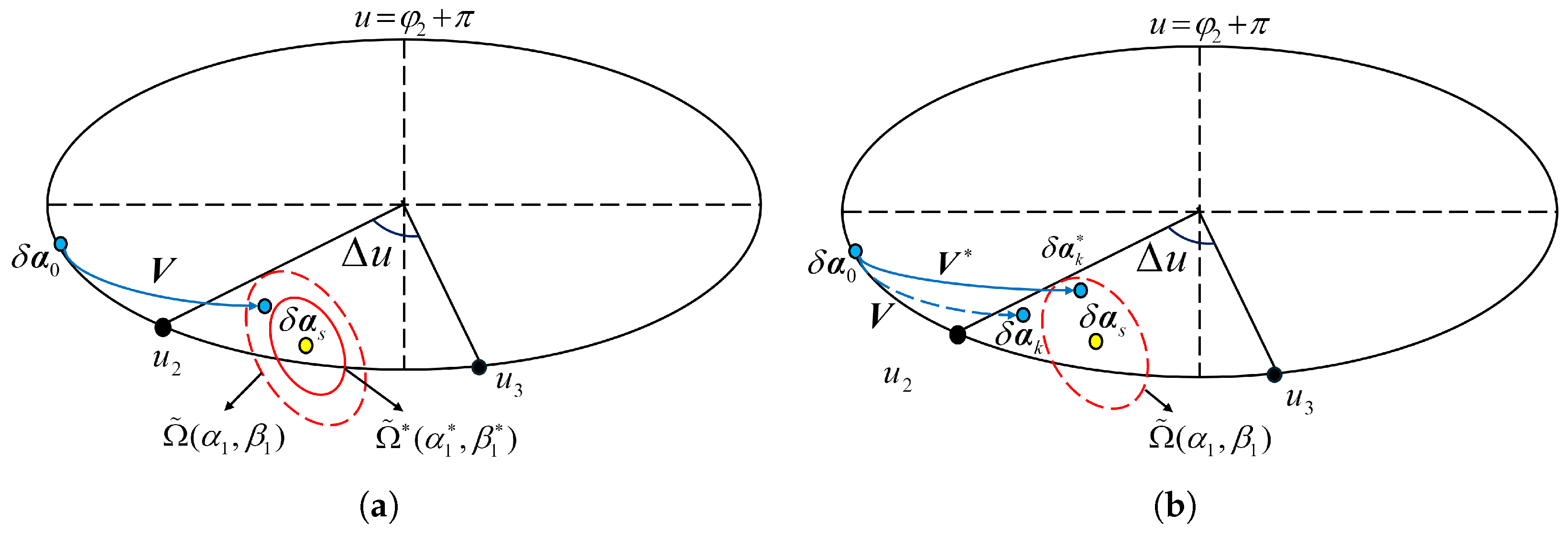
Next, to improve the flexibility and convergence of the solution and to avoid situations in which the problem has no solution due to excessively strong constraints, inspired by [25,26], the elliptical terminal set centered on the separation state δ α s , i is defined as
Ω ˜ ( k ) = Δ δ α i δ α s T P i δ α i δ α s C i
where P i and C i determine the shape of the elliptical set. On the basis of Equation (23), and taking the boundary conditions of Equation (22) as range constraints, the adaptive parameters α and β are incorporated ( λ 1 = 1 ), leading to the adaptive terminal set as follows (with the derivation provided in Appendix B):
C i = α k δ e s , x 0 + δ e s , y 0 k 2 + 1 P = λ 1 0 0 β · λ 1 1 + Δ λ ( t ) δ e
When the CMS performing separation maneuvers reaches this elliptical set, based on the control invariance of the terminal set [27], the SMSs can continuously optimize their maneuver sequences so that their states always tend toward δ α s .

2.5. Design of the CMS Separation Algorithm

By combining the above definitions of momentum effects and safe regions, this paper proposes an AMPC framework algorithm to solve the maneuver sequence for the CMS. The algorithm is divided into two optimization problems: OCP1 and OCP2. OCP1 uses MPC control to solve the control sequence V for the CMS to reach the terminal set Ω ˜ * ( δ α s ) ; OCP2 incorporates ADP ideas into the MPC algorithm to optimize either the control sequence V or the parameters α , β . By combining (19), the formulation of the discrete dynamics model for the entire multi-body satellite system is
δ α ( u k + 1 ) = f δ α ( u k ) , V n ( u k ) , k = Φ ( u k + 1 , u k ) δ α ( u k ) + ψ ( u k + 1 , u k ) V n ( u k ) + ω k Δ α ( u k )
The terminal set sequence can be further defined as
Ω * = Ω * ˜ ( δ α s , 1 , α 1 , β 1 ) Ω * ˜ ( δ α s , 2 , α 2 , β 2 ) Ω * ˜ ( δ α s , n , α n , β n )
The relevant constraints are defined as follows:
(1) Impulse Constraint
Considering the actual capability of thrusters, the compensation maneuver velocity of the CMS at each time step should not exceed the maximum velocity increment:
Δ v i Δ v max , i = 1 , 2 , , N
(2) Safety Constraints
The safety constraints in the MPC algorithm are defined as
L δ α i δ α j r safe
where L is the transformation matrix between the ROE framework and the inertial frame.
(3) Uniqueness Constraint
In order to ensure that each SMS is separated only once, the uniqueness constraint is defined as
k = 1 N ω k N
(4) Terminal Constraint
The terminal constraint is defined as
δ α ( k + m ) = F δ α ( k ) , V n ( k ) , k Ω * ˜ ( δ α s , α , β )
When (30) is satisfied, the CMS is considered ready for separation.

2.5.1. Solution to Multi-Impulse Optimization (OCP1)

Q · , H · , M · , R · denote the positive weighting matrices. The prediction time step is denoted as m, the current time step is denoted as k, Δ δ α ( k ) = δ α ( k ) δ α s , k denotes the CMS prediction error, and Δ δ α s ( k ) = δ α ( k + m ) δ α s ( N ) denotes the terminal state error. The terminal error cost function and state error cost function are defined as
J 1 ( δ α ( k ) ) = Δ δ α s ( k ) R 2
J 2 ( δ α ( k ) ) = i = 0 m 1 Δ v i Q 2 + Δ δ α ( k ) M 2 + ω k Δ α ( k ) H 2
The MPC objective function, derived from the dynamic model (19), is formulated as
min V n J = J 1 δ α ( k ) + J 2 δ α ( k ) s . t . δ α ( k + 1 ) = f δ α ( k ) , V n ( k ) , k δ α ( 0 ) = δ α ( k ) δ α f = δ α Ω ˜ * ( δ α s ) Δ v i v max , i = 1 , 2 , , N L δ α i δ α j r safe k = 1 N ω k N
The impulse sequence is derived from (33), while only the first maneuver is considered in the dynamic iteration:
δ α ( k + 1 ) = f ( δ α ( k ) , V n ( 1 ) , k )

2.5.2. Adaptive Terminal Dynamic Programming Problem (OCP2)

The value functions corresponding to the cost functions J 1 ( δ α ( k ) ) and J 2 ( δ α ( k ) ) are defined as V 1 ( δ α ( k ) ) and V 2 ( δ α ( k ) ) , respectively. By embedding the ADP algorithm into the MPC framework with penalty terms,
Λ = δ α ( k + m ) δ α s T P i δ α ( k + m ) δ α s C i
Taking a positive constant λ , the global value function is defined as
V m δ α ( k ) = V 1 ( δ α ( k ) ) + λ Λ + V 2 ( δ α ( k ) )
Let p denote the remaining steps to the terminal time m. The optimal value function V m δ α ( k ) satisfies the following Bellman recursive equation:
V p δ α ( k + m p ) = V 1 δ α ( k + m p ) + λ Λ + V 2 δ α ( k + m p ) + V N ( k + 1 ) * δ α ( k + m p )
To reduce computational load, a neural network is employed to fit the value function. Using the basis function Φ ( · ) , the fitted value function is defined as
W 0 T Φ ( δ α ( k + m ) ) V N * ( δ α ( k + m ) ) = 0
When the weight W 0 T is obtained, the remaining weights W m k ( k = N 1 , N 2 , 0 ) are solved via value iteration:
W m k T Φ δ α ( k + m p ) = V 1 δ α ( k + m p ) + λ Λ + V 2 δ α ( k + m p ) + W p 1 T Φ δ α ( k + m p + 1 )
When (30) is satisfied, to further reduce the terminal error, set the scaling parameter σ to adjust the elliptical set parameters:
α * = σ α β * = σ β
The terminal set can be expressed as
C i * = α * C i P i * = 1 β * P i
The scaling coefficient can be obtained by fitting the minimum function value:
σ * = arg min σ W m k T Φ δ α ( k )
When Equation (30) is not satisfied, take λ = 0 and solve for the optimal control input:
V * = arg min V W m k T Φ δ α ( k )
A schematic of the ADP solution problem is shown in Figure 10.

2.5.3. MPC + ADP Algorithm Framework Design

This paper proposes an algorithm for the momentum-influenced separation of the CMS, as presented in Algorithm 1. Specifically, at each time step, when calculating control actions, based on MPC prediction results, the target maneuver sequence V * or the terminal set α * , β * is adaptively adjusted.   
Algorithm 1 Enhanced model predictive control with adaptive dynamic programming (AMPC)
Input: Target State Sequence of the SMS F , Current State δ α ( k ) , Horizon N 0 , Initial Elliptical Parameters { α 0 , β 0 } , Scaling Factor σ 0 , Time Steps t ( m ) = { k , , k + m }
Output: Optimal Control V * , Terminal State δ α f
1.
Initialization: Construct terminal set:
2.
Ω ˜ α ( N ) , β ( N ) δ α s ( N ) F
3.
Dynamic Planning: Generate initial control sequence:
4.
V DP DynamicPlan ( δ α ( k ) , F , N 0 )    
5.
Step 1: Solve Optimal Control Problem (OCP1) with ADP initialization:
6.
V 1 arg min V n J 1 ( k )    (Equation (33))
7.
subject to: V n initialized with V DP , u ( m ) = u k
8.
If  δ α ( k + m ) Ω ˜ ( α , β )  then
(a)
Compute scaling parameters: { α * , β * } (Equation (40))
(b)
Solve ADP problem: V * V 2 * via ADP
9.
Else
(a)
Generate emergency maneuvers: V * (Equation (42))
10.
End If
11.
Apply control:  V * ( k )
12.
Update state:  δ α ( k + 1 ) f ( δ α ( k ) , V * ( k ) , k )
13.
Return  V * , δ α f
In summary, the safety constraints with intuitive geometric meanings are treated as terminal constraints in optimal control formulation. As shown in Figure 11, the separation of the CMS is specified as follows: the CMS travels from the initial state δ α 0 through a maneuver sequence V n to reach the stage terminal set Ω ˜ ( δ α n s , α n , β n ) .

3. Results

In this section, we validate the proposed AMPC through numerical simulations and compare its performance with that of MPC-based simulations, which consider the safety separation constraints in the AMPC framework. This section mainly conducts simulation verification within the ROE framework (Section 3.1) and the absolute coordinate system (Section 3.2). Table 1 presents the initial states of the reference satellite and the CMS, as well as the desired states of the sub-satellites.

3.1. Analysis Within the ROE Framework

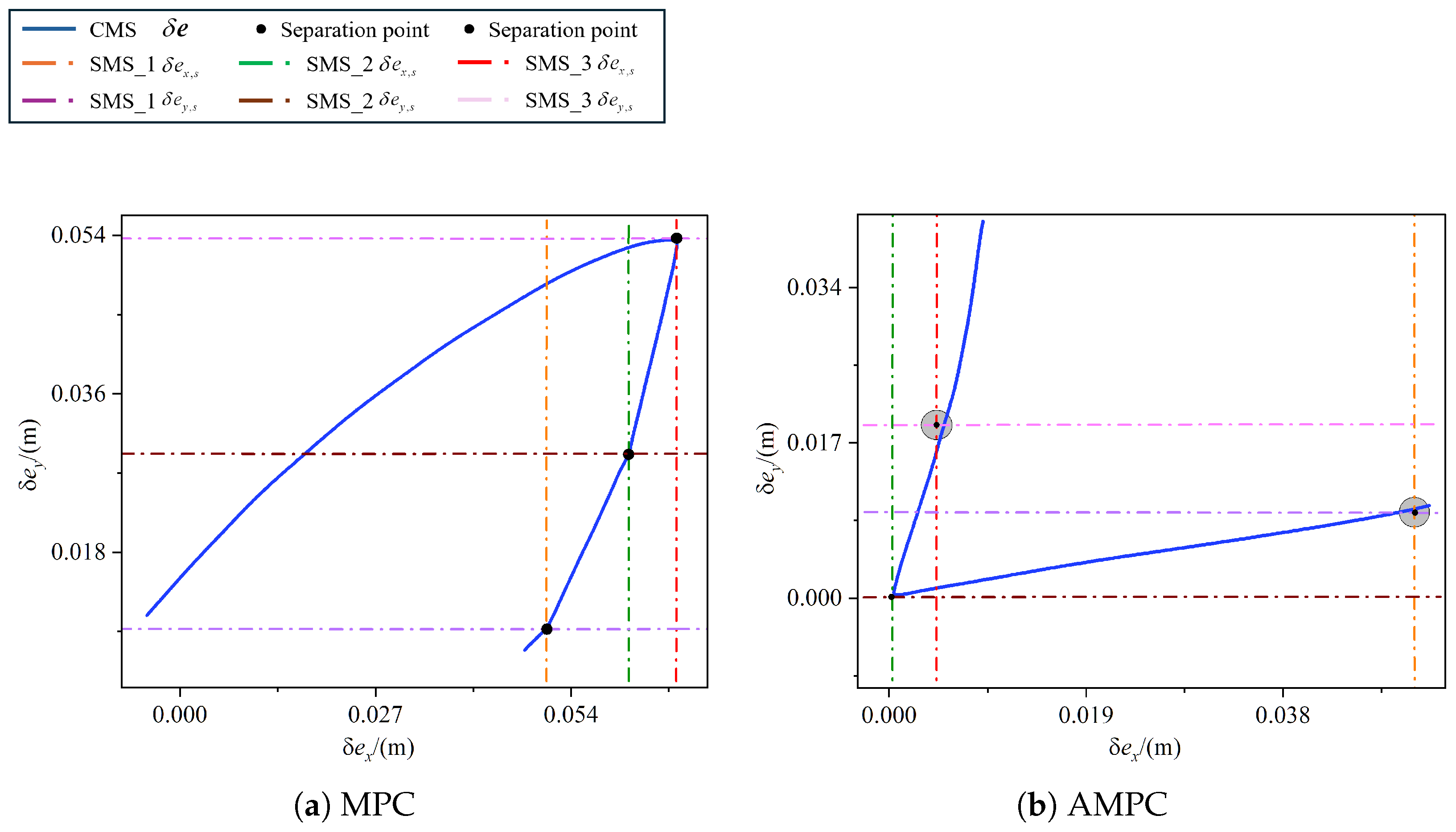
Figure 12 shows that both algorithms allow the CMS to reach the expected separation point or safe separation region.Herein, the gray areas denote the safe separation zones. Compared with MPC, AMPC realizes the safe separation of SMSs within a specific error margin under the constraints of safe separation, circumventing high-precision calculations and decreasing the computational load.
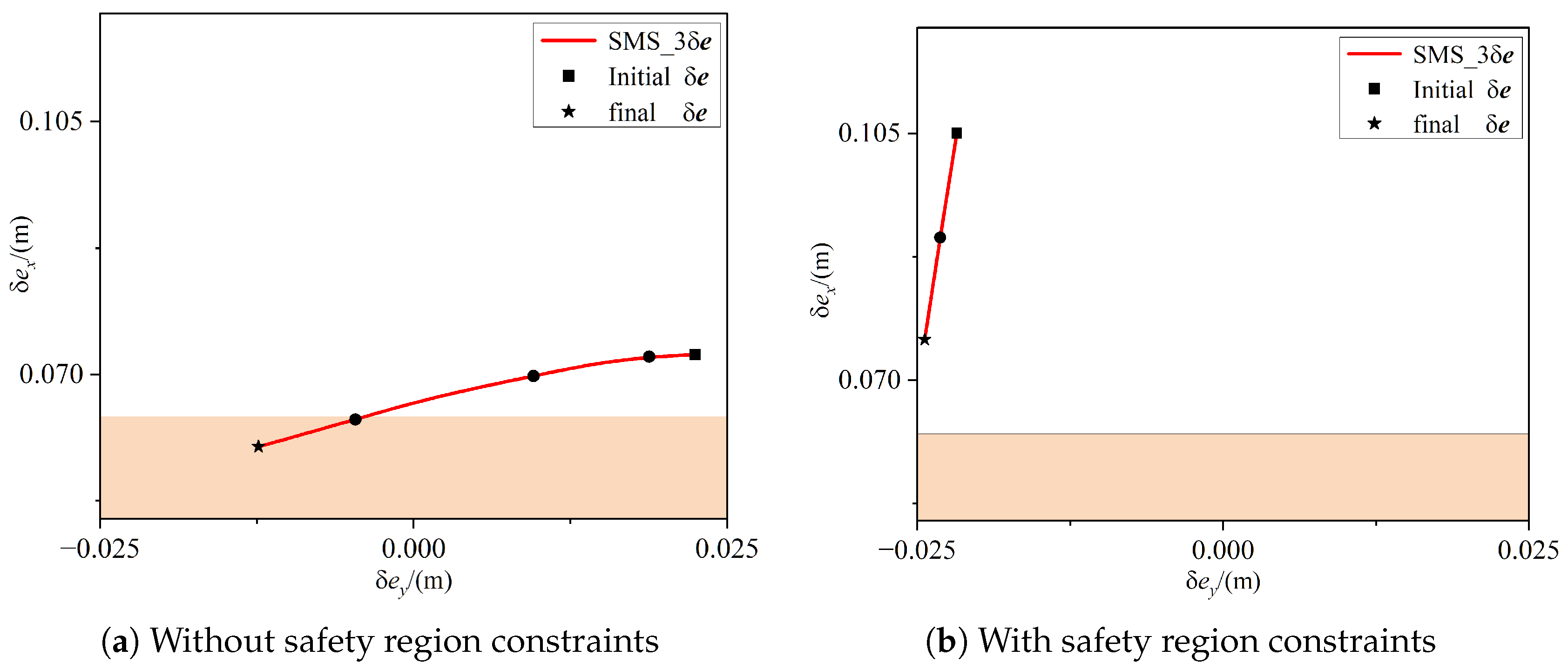
Figure 13 shows diagrams of the ROE of SMS_3 within one orbital period after separation, established with SMS_2 as the reference satellite, including cases with or without the safety region constraint. As can be seen in Figure 13b, when there is a safety region constraint, the separated SMS_3 remains within the safety region.

3.2. Analysis Within the Absolute Coordinate System

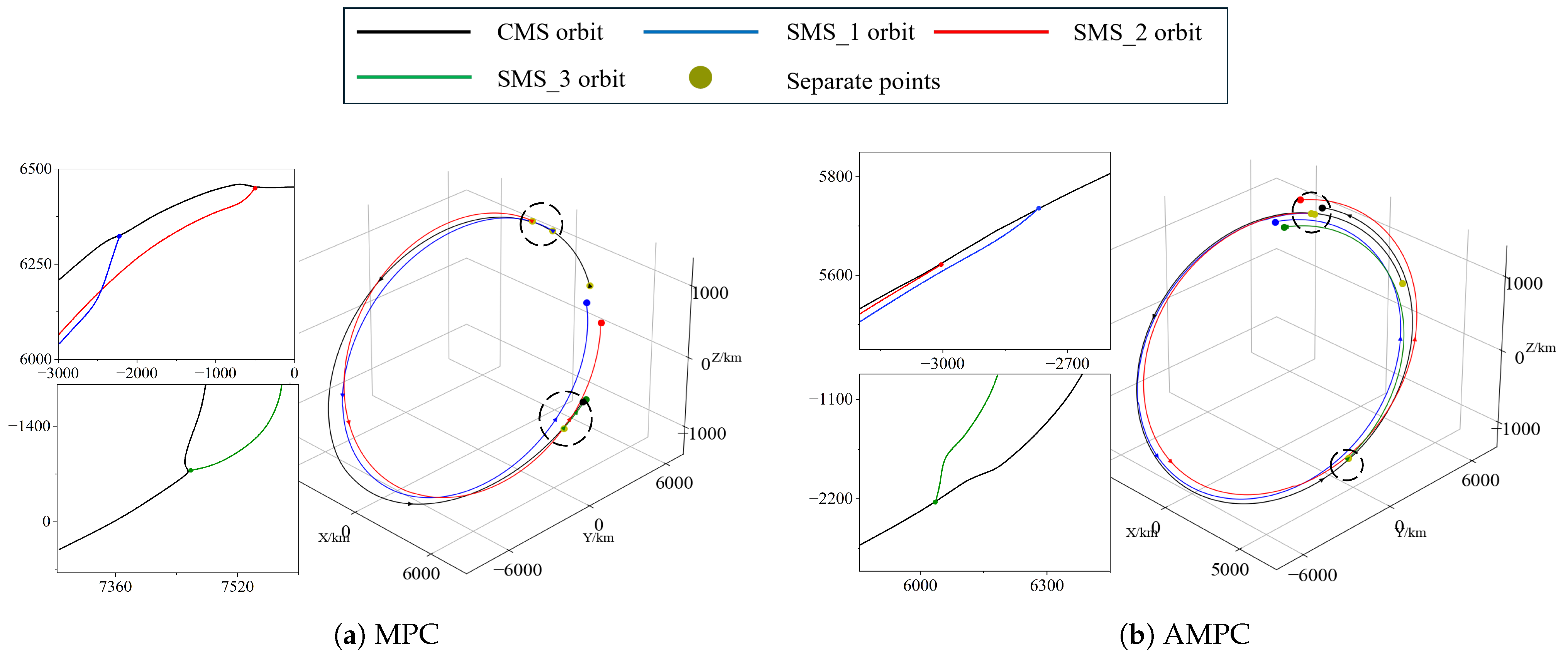
In order to illustrate the influence of momentum on the orbital altitude, Figure 14 shows the trajectories under the two algorithms. Figure 12 and Figure 14 verify that both algorithms successfully accomplish the separation tasks for the CMS. Taking the MPC simulation results as a reference point, the separation time between SMS_1 and SMS_2 is only 0.03 orbital periods. Elliptic set safety constraints are defined in AMPC, allowing separation once the relevant safety conditions are met. When the two satellites are separated simultaneously in the simulation. In the separation process of SMS_3, due to the continuous optimization of the elliptic set parameters by AMPC, its separation speed is increased by 0.14 orbital periods compared with MPC.
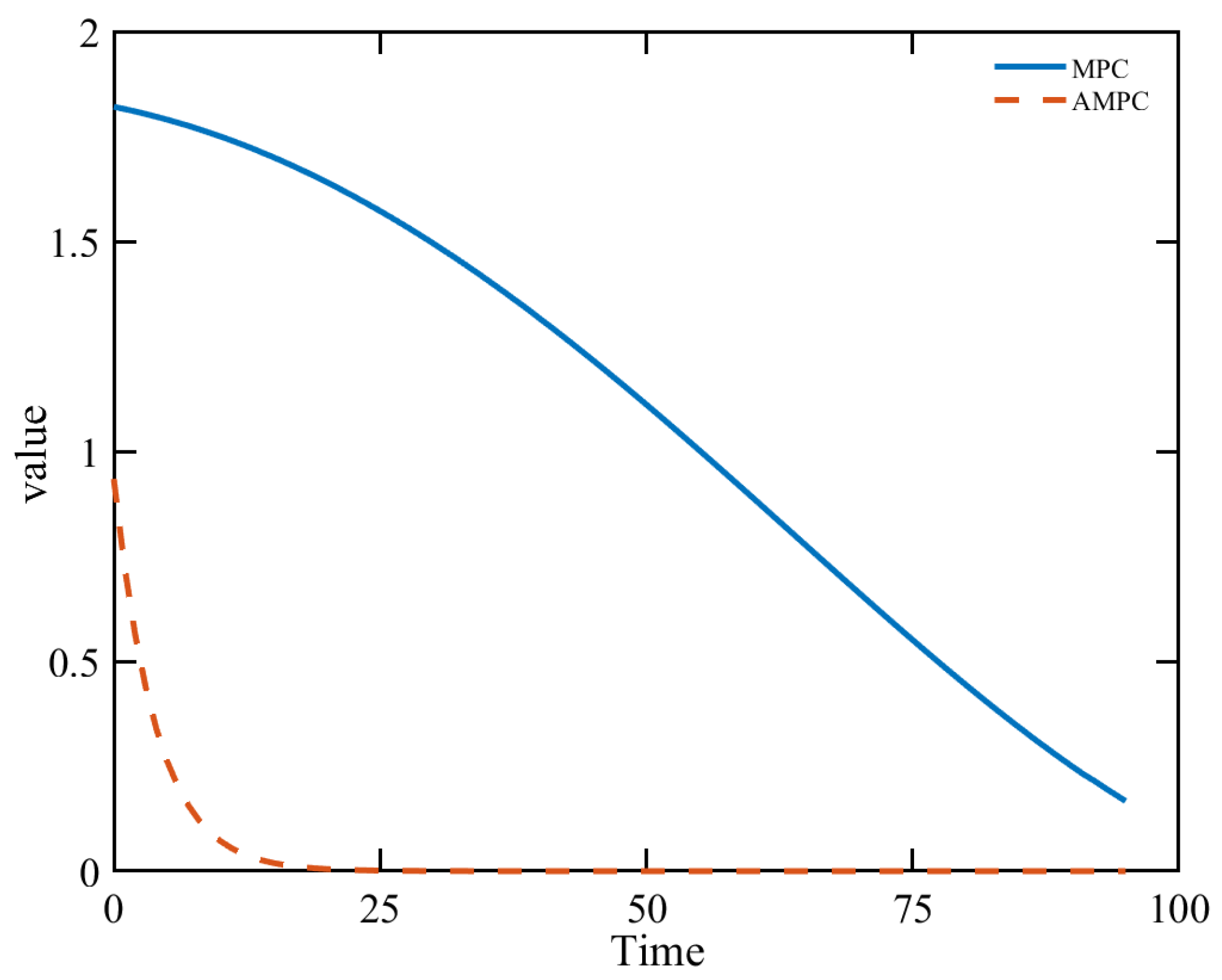
Figure 15 illustrates the variation trend of Equation (33), which quantifies the payoff function values, for the two algorithms from the separation of the second satellite to that of the third satellite. Compared with traditional MPC, AMPC significantly improves the convergence performance of the control system by introducing an adaptive mechanism. Specifically, it features a faster convergence rate (with convergence achieved at 25 s), a smoother convergence process, and convergence to a precision level much closer to zero, which indicates that the separation state α s is attained. This verifies the effectiveness of the designed adaptive strategy in enhancing the dynamic response and steady-state accuracy of the system.
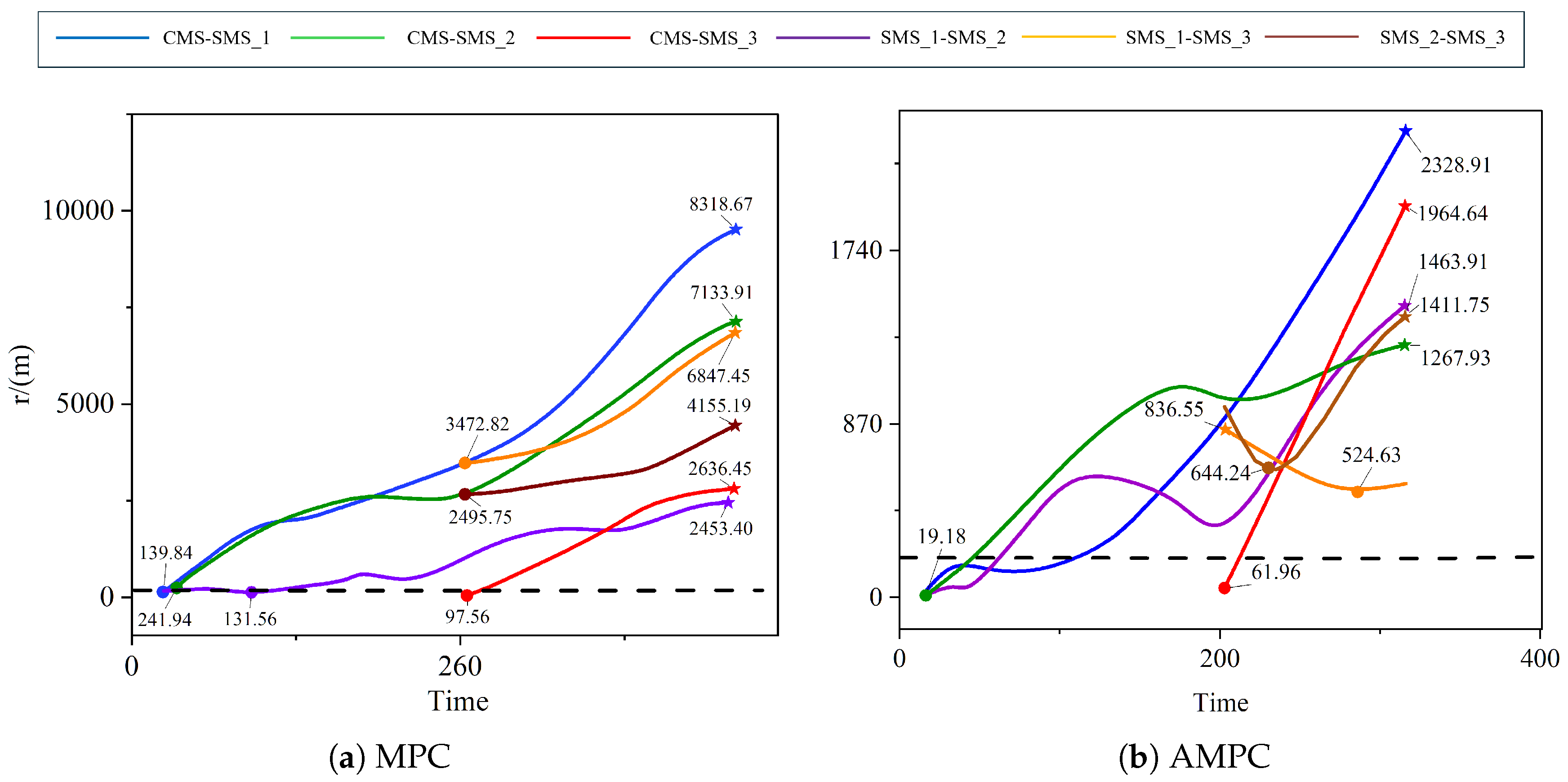
Figure 16 presents the variation in the relative distances. Under MPC, the relative distances of each satellite increase steadily; however, when separating SMS_2, the relative distance crosses the safety distance threshold, indicating that the control capability of the safety distance constraints designed in MPC is limited. Under AMPC, the relative safety distance constraints during separation and flight are ensured, and the relative distances of each satellite are stable after SMS_3 separation, indicating that the selection of separation positions is effective.
Next, we analyze the influence exerted by momentum changes. As shown in Table 2, when conducting the separation of SMS_1 and SMS_2, AMPC reduces the magnitude of the orbital altitude impact by nearly 78.4% compared with MPC, while for SMS_3 separation, the reduction rate reaches 67.2%. This proves that the penalty term ω k Δ α k H 2 added to the optimization algorithm can effectively mitigate the orbital altitude disturbance caused by the separation process. In contrast, with similar fuel consumption, AMPC saves 19.4% of the separation mission time while reducing orbital altitude variation by 78.4%, demonstrating the superiority of this algorithm.

4. Discussion

Simulation results demonstrate the effectiveness of the proposed AMPC algorithm in addressing multi-body satellite separation challenges. The key findings are discussed in two main aspects: safety separation constraints within the ROE framework and the performance of the AMPC algorithm.

4.1. Safety Separation Constraints in ROE Framework

The analysis of separation strategies within the ROE framework revealed crucial insights for multi-body satellite operations. Through numerical simulations examining different v t / v r velocity component ratios, orbital configuration variations, and separation at different arguments of latitude, we established that tangential-dominant separation ( + v t ) within the argument of latitude intervals [ 0 , π / 2 ] and [ π / 2 , 3 π / 2 ] enables the SMS and the CMS to maintain safe relative distances through orbital drift. This finding provides a fundamental principle for separation strategy design when no specific orbital configuration requirements exist for the CMS.
Building upon this foundation, the geometrically derived adaptive terminal set serves as the maneuvering target for each mission phase of the CMS. This innovative approach effectively integrates the geometrically intuitive ROE framework with the multi-dimensional optimization capabilities of MPC algorithms, overcoming previous limitations in handling complex separation constraints while maintaining clear physical interpretations.

4.2. Performance of AMPC Algorithm

The adaptive model predictive control (AMPC) algorithm exhibits substantial performance enhancements relative to conventional model predictive control (MPC) methodologies. A 78.4% reduction in orbital altitude variation underscores the paramount significance of incorporating momentum coupling effects into the design of satellite separation missions. This performance gain stems from the penalty term integrated into the optimization objective function, which explicitly mitigates momentum-induced disturbances during separation maneuvers. Additionally, the adaptive characteristic of the safety region contributes to this improvement by enabling precise calibration of separation timing and spatial positioning, thereby minimizing perturbative effects on the chief satellite (CMS) orbit. Furthermore, the 19.4% reduction in mission duration achieved by AMPC underscores its operational efficacy in autonomous spacecraft systems, where persistent human oversight is often impractical. This attribute renders the AMPC approach particularly well-suited for unmanned space operations, marking a notable stride toward the realization of fully autonomous satellite separation architectures. The fusion of geometrically interpretable safety constraints with optimal control frameworks, coupled with neural network-driven numerical solution methodologies, yields a holistic design paradigm that reconciles computational efficiency with physical interpretability. This integrated approach addresses core challenges in the design of multi-body satellite separation missions, bridging the gap between theoretical optimal control and practical aerospace engineering implementation.

5. Conclusions

In this study, an algorithm for multi-body satellite separation under the influence of momentum is proposed, which combines ADP with MPC based on adaptive safety region constraints. Unlike existing algorithms, the proposed algorithm integrates geometrically meaningful E/I vector safety constraints with optimal control as terminal conditions. A neural network is applied for numerical solutions to avoid complex E/I vector parameter variations. The resulting maneuvers are concentrated early in the task to eliminate the need for subsequent solves. This reduces onboard resource consumption, making it suitable for unmanned spacecraft deployment. Furthermore, under equivalent fuel consumption, the algorithm achieves objectives faster and mitigates the impact of momentum on orbital altitude compared to conventional methods, thereby enhancing mission reliability and efficiency.

6. Patents

This research has led to the development of novel algorithms for multi-body satellite separation. Patent applications covering the adaptive model predictive control framework with safety region constraints are currently under preparation.

Author Contributions

Conceptualization, C.Y. and L.X.; methodology, C.Y. and S.L.; software, C.Y. and L.L.; validation, R.W. and L.X.; formal analysis, C.Y.; investigation, S.L.; resources, L.L.; data curation, R.W.; writing—original draft preparation, C.Y.; writing—review and editing, L.X. and S.L.; visualization, L.L.; supervision, R.W.; project administration, C.Y.; funding acquisition, C.Y. All authors have read and agreed to the published version of the manuscript.

Funding

This research received no external funding.

Institutional Review Board Statement

Not applicable.

Informed Consent Statement

Not applicable.

Data Availability Statement

The data presented in this study are available on request from the corresponding author. The data are not publicly available due to privacy restrictions.

Acknowledgments

The authors would like to thank the anonymous reviewers for their valuable comments and suggestions that helped improve the quality of this manuscript.

Conflicts of Interest

The authors declare no conflicts of interest.

Appendix A. Derivation of the Argument of Latitude Constraint

The state of the SMS is defined with subscript 1, and the state of the CMS is defined with subscript 2. Given the argument of latitude u 1 at the moment of separation, the post-separation states of the SMS and CMS are δ α 1 and δ α 2 , respectively.
The maneuver functions for the SMS and the CMS are defined as
f ( u φ 1 ) = y = a δ a 1 δ e 1 cos ( u φ 1 ) x = a δ λ 1 3 2 δ a 1 u + 2 δ e 1 sin ( u φ 1 )
g ( u φ 2 ) = y = a δ a 2 δ e 2 cos ( u φ 2 ) x = a δ λ 2 3 2 δ a 2 u + 2 δ e 2 sin ( u φ 2 )
Equations (A1) and (A2) are transcendental equations. If an attempt is made to solve them simultaneously to find the intersection points, it is likely that only one solution or no solution can be obtained. Therefore, as illustrated in the figure, a rectangular safety zone with length L and height D is defined on the SMS after separation. Safe separation can be achieved as long as there is no intersection between this rectangle and the CMS.
Figure A1. Definition and analysis of safety constraints.
Aerospace 13 00672 g0a1
The difference in the argument of latitude between the two separations is denoted as Δ u , where the upper and lower limits of the value range of Δ u represent the safe separation range. Its lower limit is determined by satisfying the rectangular constraint, and its upper limit corresponds to one orbital period. Two solution approaches are proposed:
(1) Solve the coordinate expression of the matrix boundary based on point B, then combine it with the extremum constraint condition of the ellipse Equations ((A1) and (A2)) in the specified direction to derive the value range of the target variable.
(2) When condition D , L < < a δ a is satisfied, approximate the arc length l A B as the line segment length s A B : l A B s A B . The value range of Δ φ 1 , s a f e is derived by solving the condition s A B D 2 + L 2 .
The first approach requires extensive complex computations and strict constraint formulations, which may not yield analytical solutions in certain parameter ranges. The second approach employs approximation methods, necessitating the introduction of safety thresholds in subsequent processing to refine the constraints.
The solution process for the second approach is as follows:
(1) Establish the arc-length approximation formula:
s = a 0 Δ φ 1 , safe 9 4 δ a 1 2 3 δ a 1 δ e 1 cos θ + 4 δ e 1 2 d θ a · Δ φ 1 , safe · 9 4 δ a 1 2 3 δ a 1 δ e 1 + 4 δ e 1 2
(2) Substitute the constraint conditions:
a · Δ φ 1 , safe · 9 4 δ a 1 2 3 δ a 1 δ e 1 + 4 δ e 1 2 D 2 + L 2
(3) Solve the inequality and consider orbit drift:
Δ φ 1 , safe D 2 + L 2 a · 9 4 δ a 1 2 3 δ a 1 δ e 1 + 4 δ e 1 2
(4) Consider the orbit drift amount Δ λ ( t ) , and the influence of orbit drift on the argument of latitude is approximated as
Δ u λ = ε · arctan Δ λ ( t ) Δ e
where Δ e = e R 2 + e T 2 .
By combining the above equations, the value range of Δ u is obtained as
Δ u K 1 + Δ u λ , φ 2 + Δ u λ
where K 1 = D 2 + L 2 a · 9 4 δ a 1 2 3 δ a 1 δ e 1 + 4 δ e 1 2 .

Appendix B. Derivation of the Terminal Set

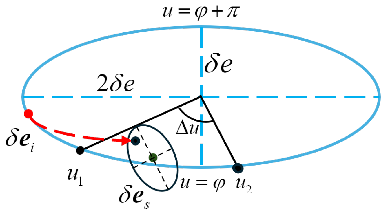
Establish a coordinate system with the center of the relative orbit of the CMS as the origin, where the horizontal axis is u = φ 2 + π 2 and the vertical axis is u = φ 2 . From the previously defined argument of latitude constraint Δ u , let us define the target state δ e s = δ e s , x 0 , δ e s , y 0 and the initial state δ e i = δ e i , x 0 , δ e i , y 0 of the CMS.
The state elliptical set Ω ˜ ( k ) is defined as
Ω ˜ ( k ) = Δ P i , C i δ e i δ e s T P i δ e i δ e s C i
As shown in Figure A2, the size of the elliptical set Ω ˜ ( k ) is combined with the argument of latitude constraint (Equation (A7)), and its boundary equation is defined as
y 1 = k 1 x 1 , k 1 = tan u 1 + K 1 + arctan Δ λ ( t ) δ e φ 2 π 2 = Δ λ ( t ) δ e cot ( u 1 + K 1 φ 2 ) 1 + Δ λ ( t ) δ e cot ( u 1 + K 1 φ 2 )
y 2 = k 2 x 2 , k 2 = tan φ 2 + arctan Δ λ ( t ) δ e φ 2 π 2 = Δ λ ( t ) δ e
Figure A2. Definition of terminal-set constraints.
Aerospace 13 00672 g0a2
The shortest distance d min from the center point to the black line is
k = arg min i 1 , 2 k 1 δ e s , x 0 + δ e s , y 0 k 1 2 + 1 , k 2 , δ e s , x 0 + δ e s , y 0 k 2 2 + 1
d min = k δ e s , x 0 + δ e s , y 0 k 2 + 1
The shortest distance d min is taken as the semi-major axis of the ellipsoidal set. The constraint of the elliptical set can thus be expressed as
C i = α k δ e s , x 0 + δ e s , y 0 k 2 + 1 P = λ 1 0 0 β · λ 1 1 + Δ λ ( t ) δ e
where α , β are the adaptive adjustment parameters.

References

  1. Luo, C.; Sun, J.; Wen, H.; Jin, D. Autonomous separation deployment dynamics of a space multi-rigid-body system with uncertain parameters. Mech. Mach. Theory 2023, 180, 105175. [Google Scholar] [CrossRef]
  2. Luo, C.; Sun, J.; Wen, H.; Hu, H.; Jin, D. Research on separation strategy and deployment dynamics of a space multi-rigid-body system. Chin. J. Theor. Appl. Mech. 2020, 52, 503–513. [Google Scholar]
  3. Liao, D.; Pan, X.; Wei, Z.; Chen, T. Assembly and reconfiguration of space structure using heterogeneous satellite swarms. Acta Astronaut. 2025, 229, 166–180. [Google Scholar] [CrossRef]
  4. Zhihui, X.; Jinguo, L.; Chenchen, W.; Yuchuang, T. Review of in-space assembly technologies. Chin. J. Aeronaut. 2021, 34, 21–47. [Google Scholar] [CrossRef]
  5. Bandyopadhyay, S.; Foust, R.; Subramanian, G.P.; Chung, S.-J.; Hadaegh, F.Y. Review of formation flying and constellation missions using nanosatellites. J. Spacecr. Rocket. 2016, 53, 567–578. [Google Scholar] [CrossRef]
  6. Chen, T.; Shan, J.; Wen, H.; Xu, S. Review of attitude consensus of multiple spacecraft. Astrodynamics 2022, 6, 329–356. [Google Scholar] [CrossRef]
  7. Wijayatunga, M.C.; Armellin, R.; Holt, H.; Pirovano, L.; Lidtke, A.A. Design and guidance of a multi-active debris removal mission. Astrodynamics 2023, 7, 383–399. [Google Scholar] [CrossRef]
  8. Jin, D.; Ding, D.; Wu, L.; Wen, H.; Zhang, X.; Sun, J. Key technologies and prospects for separation dynamics of stacked satellite systems. Acta Aeronaut. Astronaut. Sin. 2025, 46, 316–341. [Google Scholar]
  9. Sun, J.; Zhang, X.; Jin, D. Separation and reconfiguration dynamics of stacked satellites. Appl. Math. Mech. 2024, 45, 1–11. [Google Scholar]
  10. Wang, Z.; Xu, Y.; Jiang, C.; Zhang, Y. Self-organizing control for satellite clusters using artificial potential function in terms of relative orbital elements. Aerosp. Sci. Technol. 2019, 84, 799–811. [Google Scholar] [CrossRef]
  11. Miñán, A.M.; Scala, F.; Colombo, C. Manoeuvre planning algorithm for satellite formations using mean relative orbital elements. Adv. Space Res. 2023, 71, 585–603. [Google Scholar] [CrossRef]
  12. Li, S.; Ye, D.; Xiao, Y.; Sun, Z. Robust distributed model predictive control for satellite cluster reconfiguration with collision avoidance. Aerosp. Sci. Technol. 2022, 130, 107917. [Google Scholar] [CrossRef]
  13. Pippia, T.; Preda, V.; Bennani, S.; Keviczky, T. Reconfiguration of a satellite constellation in circular formation orbit with decentralized model predictive control. arXiv 2022, arXiv:2201.10399. [Google Scholar] [CrossRef]
  14. Menegatti, D.; Giuseppi, A.; Pietrabissa, A. Model predictive control for collision-free spacecraft formation with artificial potential functions. In Proceedings of the 2022 30th Mediterranean Conference on Control and Automation (MED), Vouliagmeni, Greece, 28 June–1 July 2022; pp. 564–570. [Google Scholar]
  15. Fang, H.; Zhang, R.; Wang, J.; Wang, D.; Guo, H. Injected transfer orbit determination of lunar probe Chang’E 5T1 using short-arc rocket GPS measurements. Adv. Space Res. 2015, 56, 1726–1736. [Google Scholar] [CrossRef]
  16. Gaias, G.; Ardaens, J.-S. Design challenges and safety concept for the AVANTI experiment. Acta Astronaut. 2016, 123, 409–419. [Google Scholar] [CrossRef]
  17. Peters, T.V.; Noomen, R. Linear Cotangential Transfers and Safe Orbits for Elliptic Orbit Rendezvous. J. Guid. Control Dyn. 2021, 44, 732–748. [Google Scholar] [CrossRef]
  18. Liu, P.; Chen, X.; Zhao, Y. Safe deployment of cluster-flying nano-satellites using relative E/I vector separation. Adv. Space Res. 2019, 64, 964–981. [Google Scholar] [CrossRef]
  19. Wang, J.; Ren, Y.; Zeng, Q.; Zhang, C.; Zhang, J. Relative E/I vector-based optimal and suboptimal control for continuous low thrust formation reconfiguration in circular orbits. Aerosp. Sci. Technol. 2024, 150, 109237. [Google Scholar] [CrossRef]
  20. Roychowdhury, D.; Grau, S.; Stoll, E. Helix orbit deployment of nanosatellites for formation flight: Strategy, GNSS/TLEs evaluation, and accuracy analysis. Acta Astronaut. 2025, 232, 244–257. [Google Scholar] [CrossRef]
  21. Koenig, A.W.; D’Amico, S. Safe spacecraft swarm deployment and acquisition in perturbed near-circular orbits subject to operational constraints. Acta Astronaut. 2018, 153, 297–310. [Google Scholar] [CrossRef]
  22. D’Amico, S.; Ardaens, J.-S.; Gaias, G.; Benninghoff, H.; Schlepp, B.; Jørgensen, J.L. Noncooperative rendezvous using angles-only optical navigation: System design and flight results. J. Guid. Control Dyn. 2013, 36, 1576–1595. [Google Scholar] [CrossRef]
  23. Wang, J.; Xu, C.; Zhang, C.; Zhang, J. Passive safety-constrained impulsive maneuvers for formation reconfiguration: An analytic solution. Aerosp. Sci. Technol. 2025, 158, 109901. [Google Scholar] [CrossRef]
  24. Xu, C.; Zhang, C.; Wang, J. Analytic solution for combined in-plane and out-of-plane spacecraft formation reconfiguration with passive collision avoidance. Acta Astronaut. 2025, 226, 48–59. [Google Scholar] [CrossRef]
  25. Heydari, A. Optimal impulsive control using adaptive dynamic programming and its application in spacecraft rendezvous. IEEE Trans. Neural Netw. Learn. Syst. 2020, 32, 4544–4552. [Google Scholar] [CrossRef]
  26. Li, Q.; Dai, L.; Yang, H.; Sun, Z.; Xia, Y. Economic model predictive control with terminal set dynamic programming for tracking control. Int. J. Robust Nonlinear Control 2023, 33, 5624–5644. [Google Scholar] [CrossRef]
  27. Simon, D.; Löfberg, J.; Glad, T. Reference tracking MPC using dynamic terminal set transformation. IEEE Trans. Autom. Control 2014, 59, 2790–2795. [Google Scholar] [CrossRef]
Figure 1. Schematics of the CMS, the SMS, and the multi-body satellite formation after separation.
Aerospace 13 00672 g001
Figure 2. Relative motion of the CMS in the LVLH coordinate system.
Aerospace 13 00672 g002
Figure 3. Schematic of the CMS separation mission.
Aerospace 13 00672 g003
Figure 4. Diagram of momentum analysis for CMS separation.
Aerospace 13 00672 g004
Figure 5. Comparison of radial and tangential velocity components during separation.
Aerospace 13 00672 g005
Figure 6. Effect of velocity ratio on relative distance during separation.
Aerospace 13 00672 g006
Figure 7. Effect of argument of latitude on post-separation relative motion.
Aerospace 13 00672 g007
Figure 8. Schematic of successive separation timing for the CMS.
Aerospace 13 00672 g008
Figure 9. Effect of separation interval on relative distance.
Aerospace 13 00672 g009
Figure 10. Schematic of the ADP solution framework. (a) Elliptical set Equation (23) satisfied: solve for σ * ; (b) Elliptical set Equation (23) unsatisfied: solve for V * .
Aerospace 13 00672 g010
Figure 11. Illustration of the terminal set-based separation process of the CMS.
Aerospace 13 00672 g011
Figure 12. Target-tracking trajectories of the ROEs for the CMS.
Aerospace 13 00672 g012
Figure 13. ROE trajectories with and without safety region constraints.
Aerospace 13 00672 g013
Figure 14. Trajectories of the CMS under the two algorithms.
Aerospace 13 00672 g014
Figure 15. Payoff function variation for the two algorithms.
Aerospace 13 00672 g015
Figure 16. Relative distance variation of each satellite under MPC and AMPC.
Aerospace 13 00672 g016
Table 1. Six orbital elements of satellites.
Spacecrafta/kmei/deg Ω /deg ω /degf/deg
Chief6628.140.00051020300
CMS6928.140.000110202020
SMS_17178.140.000230309030
SMS_27378.140.0002504028040
SMS_37578.140.0002703016070
Table 2. Comparison of MPC and AMPC for satellite separation.
SatelliteAlgorithm Δ v (m/s) Δ a (km)Separation Time (Orbit)
SMS_1MPC0.061541.610.12
AMPC0.05814.580.15
SMS_2MPC0.100027.710.15
AMPC0.10002.560.152
SMS_3MPC0.200070.110.72
AMPC0.200022.970.58
TotalMPC0.4788139.42
AMPC0.452530.11
Disclaimer/Publisher’s Note: The statements, opinions and data contained in all publications are solely those of the individual author(s) and contributor(s) and not of MDPI and/or the editor(s). MDPI and/or the editor(s) disclaim responsibility for any injury to people or property resulting from any ideas, methods, instructions or products referred to in the content.