


Abstract
Existing unmanned aerial vehicle (UAV) urban logistics planning follows a sequential paradigm—depot siting first, routing second—that embeds a structural information loss. Straight-line distance screening systematically overestimates the feasible service radius of candidate depots, creating a blindzone of depot–demand pairs that appear reachable but prove operationally infeasible under road network distances. We term this range-feasibility blindness and derive its analytical radius , where is the road-to-straight-line distance ratio. Empirical measurement across three Chinese urban districts confirms and blindzone radii exceeding 2.8 km, establishing the phenomenon as a systemic property of high-density urban road geometry. To eliminate this failure by construction, we formulate a feasibility-embedded location–routing mixed-integer linear programme (MILP) that enforces road network range constraints simultaneously with depot opening decisions, making blindzone configurations implicitly inadmissible. A structure-aware Adaptive Large Neighbourhood Search (ALNS) solves the model at practical scales. Benchmark experiments on Dongli District (Tianjin) show cost reductions of 20.6–28.2% over greedy sequential baselines across three demand scenarios, with gains increasing monotonically with instance scale; cross-city experiments in Beijing and Shanghai confirm consistent improvement averaging 11.4% (Chaoyang, Beijing) and 10.2% (Pudong, Shanghai) over greedy initialisation across diverse urban morphologies. These results position joint optimisation as a necessary methodological shift for city-scale UAV infrastructure planning.
1. Introduction
China’s low-altitude economy is expanding rapidly, and landing-pad siting is being institutionalised as a discrete planning phase that precedes route operations. Shenzhen has published a dedicated vertiport layout plan targeting over 1500 landing sites by 2035 under a three-tier location hierarchy [1]; Jiangsu has issued the first provincial-level guideline specifying vertiport siting principles and procedures [2]; Zhuhai has introduced a new land-use category exclusively for low-altitude landing infrastructure to formalise the siting process [3]; and Guizhou Province has mandated the systematic planning and layout of vertiports and unmanned aerial vehicle (UAV) landing points as a discrete infrastructure task, prioritising key logistics hubs before any operational routing is addressed [4]. In each case, depot location is treated as a prerequisite infrastructure decision, completed before operational routing is considered. The growing importance of UAV infrastructure siting has also attracted academic attention: Recent studies have examined vertiport network planning and capacity optimisation for UAM systems [5,6], and infrastructure-oriented work emphasises that vertiport placement critically shapes operational accessibility and network performance [7,8]. Throughout this paper, we use the term depot to refer to UAV dispatch facilities generically, encompassing vertiports and landing pads as defined in Chinese regulatory documents. This sequential paradigm (select depot locations first, optimise routes second) is equally prevalent in the research literature: existing location–routing models predominantly commit to facility configurations via straight-line (Haversine) screening before any routing constraints are considered [9,10,11,12], making it a structural property of decoupled architectures that routing infeasibility cannot propagate upward to inform location decisions.
To illustrate this failure, consider the UAV delivery planning scenario examined in this paper. In Dongli District, Tianjin, depot D0008 is selected by any straight-line-based location method (including the p-median, coverage, and proximity heuristics that dominate the existing literature [9,10,11,13]) because its aggregate Haversine distance to a cluster of eastern demand nodes is low and it passes every straight-line feasibility check. Yet when road network routing is attempted, an industrial zone forces a substantial detour (making the actual flight distance approximately 3.4 km longer than the straight-line approximation), and D0008 proves operationally infeasible. This failure is not a planning error; it is a structural consequence of treating location and routing as separable decisions.
The regulatory framework for UAV urban operations in China is still evolving. Current regulations require operators to file flight routes for approval but do not prescribe how urban delivery corridors should be structured. This paper adopts road network corridors as the operational basis for UAV routing. It is important to distinguish three separate claims: (i) This is an operational assumption adopted in this paper’s model, not a description of current regulatory requirements; (ii) we argue that this assumption is practically grounded in the physical and regulatory constraints of dense urban environments; and (iii) we further argue that formalising road network corridors as a planning standard is a policy-actionable design principle that regulators and planners could adopt. The three justifications below support claim (ii) and motivate claim (iii); they do not assert that current regulations already mandate this choice. Road network-referenced corridors offer three compounding advantages. Physical clearance: Arterials, rivers, and railways constitute the principal linear open spaces in dense urban morphology; setback requirements and lower building density along these corridors provide comparatively clear vertical clearance, making them the natural minimum-detour channels for obstacle avoidance. Any route departing from these corridors must either gain substantial altitude to clear rooftops (increasing energy consumption and flight time) or navigate between buildings (requiring centimetre-level obstacle avoidance infeasible at delivery scale). Regulatory tractability: Routes anchored to named roads are unambiguously specifiable and verifiable by air traffic service providers; arbitrary point-to-point geodesics through built-up areas are not. Provincial and municipal governments have already institutionalised infrastructure-first planning as a precondition for operations: Shenzhen, Jiangsu, Zhuhai, and Guizhou have each issued formal guidelines requiring systematic planning of take-off and landing sites before any operational routing is addressed [1,2,3,4]. Navigational reproducibility: The same road-referenced route can be executed consistently across hundreds of daily sorties; road network corridors are spatially continuous, publicly documented, and geometrically stable. Among existing urban infrastructure, road networks most comprehensively satisfy all three criteria simultaneously. The circuity factor that emerges from this assumption is therefore not a model artefact but an empirically measurable property of the deployment environment, and its consequences for infrastructure planning are the subject of this paper. In our measurements across 2850 node pairs in Dongli District, the road-to-Haversine ratio (circuity factor ) averages 1.52. When , Haversine pre-screening overestimates the feasible service radius by:
where is the UAV maximum flight range, and is the road-to-Haversine distance ratio. For Dongli District (, m), m. Straight-line screening therefore overestimates the feasible service radius by over 3.4 km. Depot–demand pairs falling within this blindzone, such as those between D0008 and its eastern demand nodes, appear reachable but are operationally infeasible, with infeasibility only exposed at the routing stage when the location decision is already irrevocable. We term this structural failure mode range-feasibility blindness.
Is this a local quirk of Tianjin’s road network or something more systematic? To answer this question, we conducted road network circuity measurements across three representative Chinese urban districts. In Beijing’s Chaoyang District (), m; in Shanghai’s Pudong District (), m. Every city we examined has a blindzone exceeding 2.8 km, suggesting range-feasibility blindness is a systemic planning risk across Chinese urban morphologies rather than a local anomaly.
As illustrated in Figure 1, the UAV-LRP requires jointly selecting depot sites and constructing delivery routes subject to range and payload constraints, two decisions that are tightly coupled but treated as separable under the sequential paradigm.
Figure 1.
UAV location-routing problem. From M candidate depot sites, a subset is selected (coloured stars); closed depots are shown as grey circles. Each open depot dispatches up to K drones on multi-stop routes (solid lines) to demand nodes , returning to the home depot (dashed lines). Location and routing are tightly coupled: Which depots to open constrains route feasibility, and which routes are needed shapes the optimal depot set. In the figure, green stars represent depots selected by the joint optimiser; the orange star represents the reference depot used for illustration.
Existing methods break the location–routing coupling into sequential or bilevel stages [9,10,11]: the location layer selects depots using an aggregated cost estimate, then the routing layer optimises with those locations fixed. Under road network circuity, this information loss produces infeasible depot configurations that are only discovered at the routing stage, when the location decision is already irrevocable. In UAV systems this aggregation is more damaging than in ground logistics; a small change in depot location can render demand nodes unreachable under battery-endurance constraints, yet this infeasibility produces no upward signal in a bilevel model [13,14].
The main contributions are as follows:
- Discovery and empirical quantification of range-feasibility blindness in city-scale UAV infrastructure planning. We identify that straight-line distance screening (the standard practice in both policy and research) creates a systematic blind spot, formalise it as the blindzone radius , and empirically quantify it across three Chinese cities, finding it consistently exceeds 2.8 km, regardless of urban morphology. This is not a local anomaly; it is a structural feature of how Chinese cities are built.
- Causal evidence that decoupled planning picks the wrong depots. A controlled experiment in Dongli District shows that when depot selection and routing are treated as separate decisions, the selected depot set can be operationally infeasible as well as invisible to the location criterion and only discovered when routing begins and the commitment is already irrevocable. All five independent routing runs failed. The failure is not algorithmic; it is architectural.
- A feasibility-embedded location–routing formulation that closes the blind spot by design. By enforcing road network range constraints simultaneously with depot-opening decisions in a unified mixed-integer linear programme (MILP), blindzone depots become implicitly inadmissible. The location layer no longer commits to sites that routing cannot serve, closing the structural information gap that decoupled models leave open.
- Cross-city benchmark validation demonstrating consistent improvement across three urban districts with distinct road network morphologies. Tested on real OpenStreetMap road networks in Tianjin, Beijing, and Shanghai, the feasibility-embedded framework consistently outperforms greedy initialisation across all cities and dataset types, including a 28.3% total cost reduction and 100% fleet utilisation in the full Dongli case study where the decoupled baseline fails entirely. The results suggest the framework generalises across diverse Chinese urban environments.
The remainder is organised as follows. Section 2 reviews related work. Section 3 presents the MILP formulation. Section 4 describes the ALNS framework. Section 5 reports benchmark experiments. Section 6 presents the Dongli District case study. Section 7 presents the cross-city circuity analysis and multi-city validation. Section 8 discusses practical implications and limitations. Section 9 concludes.
2. Related Work
2.1. UAV Routing and Truck–Drone Coordination
Early studies on UAV-assisted logistics primarily focused on routing optimisation under fixed depot configurations. Although recent UAM infrastructure studies have examined route network planning, node selection strategies, and city-wide air corridor design [15,16], early UAV-assisted logistics research treated depot locations as fixed inputs. The rapid growth of drone delivery research has been documented in recent surveys [17,18]. Murray and Chu [19] introduced the Flying Sidekick Travelling Salesman Problem (FSTSP), establishing one of the earliest coordinated truck–drone delivery frameworks. Dorling et al. [20] further incorporated UAV energy consumption and endurance constraints into vehicle routing problems, demonstrating the importance of battery-aware flight planning. Agatz et al. [21] proposed optimisation approaches for the Travelling Salesman Problem with Drone (TSP-D), highlighting the combinatorial complexity of synchronised truck–drone operations.
As the field evolved, Murray and Raj [22] investigated multi-drone coordination within truck-assisted delivery systems, while Kang and Lee [23] developed exact algorithms for heterogeneous truck–drone routing problems. A comprehensive survey by Boysen et al. [24] reviewed last-mile delivery concepts from an operational research perspective, encompassing drone-assisted routing structures and synchronisation challenges.
Despite these advances, most routing-oriented studies assume predetermined depots and therefore cannot capture the strategic interaction between infrastructure placement and route feasibility. Routing feasibility is typically evaluated only after facility deployment decisions have already been made, limiting the ability of these models to address infrastructure-dependent accessibility in realistic urban environments.
2.2. Joint UAV Location–Routing Optimisation
To address the limitations of fixed-depot routing models, subsequent studies introduced integrated location–routing frameworks. Hong et al. [25] investigated drone delivery service planning through range-constrained recharging station deployment and coverage optimisation, one of the earliest facility location models for drone delivery infrastructure. Bruni et al. [26] formulated a drone location–routing problem for last-mile delivery under flight-time uncertainty, integrating fulfilment-centre selection with drone routing. Zhou et al. [27] jointly optimised UAV service routes and depot locations in a multi-depot urban network using a tailored Adaptive Large Neighbourhood Search (ALNS) algorithm.
Recent studies have increasingly emphasised unified or coupled frameworks. Zandieh et al. [28] investigated integrated ground–drone routing under coupled operational constraints. Liu et al. [29] focused on joint truck–drone routing in urban environments, while bilevel formulations [9,10,14,30] allow limited location–routing interaction but compress routing information into a single aggregated cost signal. Dukkanci et al. [13] provide a comprehensive survey of facility location decisions for drone delivery.
Although these studies are commonly described as “integrated” or “joint” frameworks, many still rely on geometric distance assumptions or sequential feasibility evaluation. Recent vertiport siting studies for UAM, for instance, apply GIS-based spatial screening and geometric proximity criteria during infrastructure selection, without enforcing route-level feasibility constraints [7]. Candidate depots are first screened using Euclidean or Haversine distances, implicitly assuming that geometric proximity adequately represents operational accessibility [11,12,31]. In network-constrained urban environments, however, effective UAV accessibility may differ substantially from geometric distance due to road detours, no-fly zones, and urban network heterogeneity. Depot–demand pairs that appear feasible under geometric screening may therefore become operationally infeasible during actual routing, a gap that existing integrated studies have not addressed. In effect, existing integrated UAV logistics studies optimise geometric connectivity rather than operationally realisable accessibility, a critical gap that this paper addresses.
2.3. Solution Methodologies for UAV Logistics Optimisation
The increasing complexity of UAV location–routing problems has motivated advanced exact and heuristic approaches. Exact methods including decomposition-based frameworks have been applied to small- and medium-scale instances: Deng et al. [32] proposed a Benders decomposition framework for stochastic truck-and-drone routing problems, demonstrating the effectiveness of decomposition in handling uncertainty.
For realistic-scale instances, metaheuristic approaches have become necessary. Adaptive Large Neighbourhood Search (ALNS), originally proposed by Ropke and Pisinger [33], has been widely applied in vehicle routing due to its ability to iteratively destroy and reconstruct solution structures while maintaining scalability. Ropke and Pisinger [33] originally proposed ALNS for the pickup and delivery problem, and Pisinger and Ropke [34] subsequently generalised the framework to a broad class of vehicle routing problems, demonstrating its scalability and effectiveness across diverse logistics settings. Population-based metaheuristics such as genetic algorithms and hybrid evolutionary frameworks [35] remain widely used for combinatorial location–routing optimisation, though existing solution methodologies primarily focus on improving computational performance rather than embedding operational feasibility directly into the optimisation model. DRL-based methods have been applied to multi-UAV MINLP [36] but lack optimality guarantees and do not handle discrete facility selection.
This paper closes the gap by formulating the UAV-LRP as a feasibility-embedded location–routing optimisation in which location and routing variables coexist in one model, embedding road network range constraints directly into depot-opening decisions, and analytically characterising the feasibility blindzone that arises when straight-line screening is used in place of road network distances. In UAV systems, the information loss from decoupled architectures is more damaging than in ground logistics: A small change in depot location can render demand nodes unreachable under battery-endurance constraints, yet this infeasibility produces no upward signal in a bilevel model [9,10,14]. This makes the structural fix proposed here not merely beneficial but necessary.
3. Problem Formulation
3.1. Problem Description and Assumptions
We consider a UAV delivery system in an urban environment where a logistics operator jointly decides depot locations and drone routing. The following assumptions are adopted: (1) UAVs operate along road network corridors and return to their home depot after each mission, reflecting the practical constraint that direct overland flight in dense urban environments is often hindered by building obstruction and urban safety considerations. This assumption reflects current operational practice for urban UAV logistics in China; the framework remains valid under any distance metric, and range-feasibility blindness diminishes as in less constrained environments where direct point-to-point flight is permitted; (2) candidate depot and demand node locations are known; (3) flight feasibility is pre-screened using Haversine distance as a conservative lower bound, with road network distances used in the objective; (4) each depot has a fixed opening cost and fleet capacity K; (5) each UAV carries a full charge with payload limit Q and range limit ; (6) demand is deterministic.
Let denote candidate depots and demand nodes. The geodesic (Haversine) distance between nodes a and b is [37]
where m is the mean Earth radius. Since always holds, Haversine pre-screening is conservative; pairs excluded are genuinely infeasible, but pairs admitted may still be infeasible under road network distances—the source of the blindzone analysed in Section 7.
3.2. Model Formulation
Feasible edge sets are pre-computed: and . It is important to clarify how this Haversine pre-screening relates to the blindzone problem identified in this paper. The pre-screening uses Haversine distance as a conservative lower bound always holds, any pair excluded by the Haversine filter is genuinely road network infeasible, so no feasible pair is ever discarded. However, pairs that pass the filter may still be road network infeasible—this gap is precisely the blindzone. The distinction from sequential planning is that the range constraint (Equation (7)) is enforced using road network distances simultaneously with depot-opening decisions , not as a post-hoc routing check. Depot configurations whose road network routes violate the range budget are therefore penalised and excluded during optimisation, not discovered after the location decision is committed. The Haversine pre-screening serves only to reduce the model size by eliminating edges that are infeasible under any metric; it does not define the feasibility criterion used in the optimisation itself. The bilinear coupling is linearised exactly via McCormick auxiliary variables [38] , yielding a pure MILP. The joint objective minimises total cost (depot opening plus routing distance), formulated by the authors as
Unit normalisation.
The objective combines two cost components with different native units: depot opening costs (in CNY) and routing distances (in metres). To make these commensurable in a single objective, routing distances are converted to cost-equivalent units using a per-metre operational cost coefficient (CNY/m), so that the effective routing cost term is . In the benchmark experiments, is calibrated to produce a routing cost in the same order of magnitude as typical opening costs (2200–28,200 CNY), following the standard practice in location–routing literature of folding the unit conversion into the distance coefficients. Concretely, CNY/m is used throughout, which is consistent with the reported cost ranges: At this rate, a 10 km round-trip route contributes 10,000 CNY, comparable to the median opening cost of approximately 15,000 CNY. This value reflects the assumption that per-flight operational expenditure (energy, maintenance, and labour amortisation per sortie) is of the same order as the annualised infrastructure cost per depot; alternative calibrations rescale the cost surface but do not alter the qualitative structure of the optimal solution or the relative advantage of joint over sequential planning.
Six constraint groups enforce coverage, fleet activation, payload, flight range, flow balance, and MTZ subtour elimination. For completeness, all six groups are stated below.
- C1—Coverage. Every demand node must be served by exactly one drone from exactly one open depot:
- C2—Fleet activation. A drone route can be activated at depot i only if depot i is open, and at most K drones depart each open depot:
- C3—Payload. The total demand weight on drone k from depot i must not exceed UAV payload capacity Q:
- C4—Flight range. The total road network distance flown by drone k from depot i on a single sortie must not exceed :is the critical coupling constraint: by enforcing it simultaneously with depot-opening decisions , the formulation makes blindzone depots implicitly inadmissible.
- C5—Flow balance. Standard flow-conservation constraints ensure that each drone departs and returns to its home depot, and visits each assigned demand node exactly once:
- C6—MTZ subtour elimination. The MTZ subtour variables (indexed per depot to reflect multi-depot structure) follow the formulation of Miller, Tucker and Zemlin [39], using as the tightest valid big-M value:
The range constraint (7) is an original contribution of this paper: It is the first formulation to couple road network range limits directly with binary depot-opening decisions, making blindzone configurations implicitly inadmissible. Complete model notation is summarised in Table 1.
Table 1.
Model parameters and decision variable definitions.
3.3. Computational Complexity
The UAV-LRP is hard, as it generalises both facility location and vehicle routing, each individually hard. The dominant binary variable term scales as .
This theoretical complexity translates directly into practical intractability at moderate scales. For the D8_J50 instance (, , ), the model contains over binary variables and constraints, exhausting available RAM during Gurobi presolve. This confirms the scalability barrier for exact methods and motivates the ALNS proposed in Section 4.
3.4. Solution Approach Overview
Given the NP hardness of the problem, we adopt a structure-aware Adaptive Large Neighbourhood Search (ALNS) as the primary solution method, following the destroy-and-repair metaheuristic paradigm originally proposed by Ropke and Pisinger [33]. The ALNS maintains a complete solution at each iteration and applies probabilistically selected destroy–repair operator pairs to escape local optima.
The key algorithmic contributions over standard ALNS are (i) dimensional partitioning, where destroy operators explicitly target the location dimension (D5: Depot destroy), routing dimension (D1–D4, D6–D7), and feasibility dimension (D8: Overload removal), ensuring that the joint location–routing search space is explored systematically; (ii) feasibility-aware repair, where all repair operators enforce the road network range constraint (Equation (7)) at the point of demand reinsertion, preventing blindzone depot selections from re-entering the solution; (iii) adaptive weight updates (Equation (11)) that shift operator selection probability toward high-performing operators as the search progresses.
The acceptance criterion is simulated annealing (Kirkpatrick et al. [40]) with parameters tuned for the UAV-LRP problem class. Complete operator specifications, parameter values, and pseudocode are given in Section 4.
4. ALNS Optimisation Framework
The ALNS framework follows the destroy-and-repair paradigm. A solution is a triple where is the open depot set, assigns demand nodes to depot–drone pairs, and gives the routing sequence per drone. This unified representation enables simultaneous exploration of location and routing decisions in every iteration.
4.1. Operator Design: Dimensional Partitioning
The central design principle is dimensional partitioning: Each destroy operator targets a specific decision dimension. The three-way partitioning covers location, routing, and feasibility dimensions.
Location-targeting (D5). The Depot destroy operator closes the highest-cost open depot and releases all its demands, directly modifying .
Routing-targeting (D1–D4, D6–D7). Six operators modify demand assignment and tour structure within a fixed depot set: Random, Worst-Cost, Shaw/Related, Route, Cluster, and Tail Removal.
Feasibility-targeting (D8). The Overload operator removes demands from routes violating payload or range constraints.
Six repair operators reinsert unassigned demands: Greedy, Regret-2, Regret-3, Nearest-Depot, Random, and Cost-Saving. All operators consider opening previously unopened candidate depots when doing so reduces total cost, enabling dynamic depot-set expansion. Four local search moves (2-Opt, Relocate, Swap, Cross-Route Transfer) are applied periodically.
4.2. Adaptive Weight Update and Acceptance
Operator weights are updated every iterations following the adaptive scheme of Ropke and Pisinger [33]:
where , is accumulated score, and is usage count. Score increments reward new global best, improving accepted, and non-improving accepted moves (values tuned by the authors); weight floors of 0.1 prevent complete operator elimination.
The simulated annealing acceptance criterion follows Kirkpatrick et al. [40], with initial temperature set as and cooling rate per iteration (both parameters set by the authors for this problem class), where is the initial solution cost.
5. Computational Experiments
5.1. Experimental Setup
Nature of experiments. All experiments are computational simulations based on real geospatial data (road networks from OpenStreetMap, projected to CGCS2000 Gauss-Krüger coordinates). Physical UAV flight trials are beyond the scope of this paper, which focuses on the infrastructure planning decision (depot siting and route design) rather than UAV hardware performance. The computational experiments serve as the appropriate validation modality for a combinatorial optimisation framework: They verify solver correctness against an exact solver (Gurobi), quantify solution quality relative to alternative algorithms (GA and other metaheuristics), and assess generalisability across three cities and three demand scenarios. Physical trials would validate the UAV hardware and flight control systems, not the combinatorial planning model studied here.
To demonstrate the competitive advantage of ALNS over alternative metaheuristics beyond GA, we additionally compare against Simulated Annealing (SA) and Variable Neighbourhood Search (VNS) on seven representative instances of increasing scale (Section 5.6). All three algorithms use an identical move set and neighbourhood structure; SA uses the acceptance criterion of Kirkpatrick et al. [40] with the same temperature schedule as the ALNS component, and VNS applies the same local search operators in a deterministic descent without adaptive weights.
All experiments ran on an Intel Core i5-1135G7 (2.40 GHz, 16 GB DDR4), Windows 11. ALNS was implemented in Python 3.10; Gurobi 13.0 solved small instances (MIPGap , time limits 7200/14,400/86,400 s). ALNS used MAX_ITER , SEGMENT_SIZE , LS_FREQ , 10 independent runs per instance. The GA baseline used population 30, 300 generations, tournament .
5.2. Benchmark Dataset Design
Instances are generated from real geospatial data anchored to Dongli District, Tianjin (117.28°–117.41° E, 39.07°–39.17° N). UAV parameters: kg, m, drones per depot. Three datasets: DS1 (standard, log-normal opening costs 2200–10,400 CNY, uniform demand 0.5–3.0 kg), DS2 (high geographic density), DS3 (tripled opening costs). Nine instances span Small, Medium, and Large tiers (D3_J8 through D20_J150).
5.3. ALNS Correctness and Scalability
On small instances, ALNS matches Gurobi-optimal on D3_J8 and D4_J10 (MIPGap confirmed) and matches Gurobi’s best incumbent on D4_J12 (≈0% gap). For D5_J20, Gurobi returns no feasible solution within 48,574 s, whereas ALNS solves it in 8.6 s (std across all ten seeds). For D5_J30, ALNS finds a solution 0.04% better than Gurobi’s best incumbent; since Gurobi had not proven optimality at termination (50.25% gap), this improvement is relative to the best known incumbent. Gurobi exhausts 16 GB RAM at D8_J50 during presolve, confirming that ALNS is necessary for deployment beyond small instances. Table 2 reports the cross-validation results for small instances alongside Gurobi, and full ALNS DS1 results across all nine instances.
Table 2.
ALNS vs. Gurobi 13.0 cross-validation and full DS1 benchmark results. Gap ; negative values indicate ALNS improves upon Gurobi’s best known incumbent. LB ≤ true optimum ≤ best by definition.
5.4. Comparison with Genetic Algorithm Baseline
Table 3 compares ALNS against the GA baseline with Wilcoxon rank-sum significance tests ( runs per method). ALNS outperforms GA by an average of 13.73%, with the advantage increasing monotonically from 11.19% (D5_J20) to 16.69% (D20_J150). At all six scales the test rejects with and (perfect rank separation; every ALNS run produces a lower cost than every GA run).
Table 3.
ALNS vs. genetic algorithm with statistical significance (DS1). runs per method.
5.5. Ablation Study
Three-way ablation on the three largest instances confirms that all components are essential. Local search is the most impactful; removing it causes degradation at D20_J150. Adaptive weights provide benefit and a variance increase without them. D5 contributes structural diversity; while best-cost degradation is modest (), standard deviation nearly doubles ().
5.6. Comparison with SA and VNS
Table 4 compares ALNS against Simulated Annealing (SA) and Variable Neighbourhood Search (VNS) across seven instances spanning all three scale tiers. All three methods share the same operator pool and neighbourhood structure; the only differences are the acceptance criterion (ALNS and SA use the SA rule of Kirkpatrick et al. [40]; VNS applies deterministic descent) and operator selection (ALNS uses adaptive weights following Ropke and Pisinger [33]; SA and VNS use uniform selection).
Table 4.
ALNS vs. SA vs. VNS: solution quality and computation time. Each method run 10 times per instance; best and average costs reported. ALNS_vs_SA and ALNS_vs_VNS: percentage improvement of ALNS best over competitor best (>0 = ALNS better).
5.7. ALNS vs. LNS: Value of Adaptive Weighting
To isolate the contribution of the adaptive weight mechanism, we compare ALNS to a uniform Large Neighborhood Search (LNS) baseline that uses equal operator selection probabilities throughout. Figure 2 presents the results.
Figure 2.
ALNS vs. LNS across all nine DS1 instance scales. (a) Solution quality; (b) ALNS improvement over LNS; (c) computation time. Adaptive weights provide measurable and growing benefit at scales ≥ D5_J30.
The results reveal a clear scale-dependent pattern. For all four smallest instances (J8–J20), both algorithms find identical best solutions, demonstrating that adaptive operator selection provides no additional benefit when the search landscape is simple enough for uniform random exploration to cover it adequately.
Beginning at D5_J30, ALNS outperforms LNS, and the advantage grows monotonically with instance complexity. At D15_J100, ALNS achieves a 1.18% improvement; at D20_J150, the gap widens to 1.23%. The mechanism behind this scaling behavior is consistent with the adaptive weight theory: As instance size grows, operator performance becomes more heterogeneous, with some operators being far more effective than others for a given problem structure, and the adaptive weight mechanism shifts probability mass toward the high-performing operators, yielding better per-iteration expected improvement. Under uniform LNS, this probability mass is wasted on underperforming operators.
Regarding computation time, LNS is marginally faster on medium instances (D8_J50: 71.8 s vs. 89.3 s) due to the absence of weight update overhead, but this reverses at larger scales where ALNS’s better solution quality reduces time spent in suboptimal regions (D20_J150: 1646 s vs. 1695 s).
5.8. Cross-Dataset Generalization
To evaluate algorithm robustness, we solve all nine instances on all three datasets and compare ALNS against the greedy initialization. Figure 3 presents the results and per-instance improvement rates.
Figure 3.
ALNS vs. greedy initialization across three benchmark datasets. (a) DS1 (standard) improvement rates per instance. (b) DS2 (high demand density) improvement rates. (c) DS3 (high opening cost) improvement rates. (d) Combined improvement curves across all three datasets. DS2 and DS3 exhibit larger average improvement margins than DS1. Per-instance improvement rates by dataset are shown for all three scenario types.
Three findings emerge from the cross-dataset analysis:
First, ALNS consistently improves over greedy across all datasets and instance sizes, indicating algorithmic robustness to geospatial and cost parameter variation. Average improvement rates of 20.6% (DS1), 28.2% (DS2), and 27.3% (DS3) suggest that ALNS delivers greater benefit in more challenging scenarios.
Second, the improvement margin grows with instance scale within every dataset. On D3_J8 and D4_J10, greedy initialization already finds near-optimal solutions (0–4% improvement); by D20_J150, ALNS achieves 38.4% (DS1), 52.9% (DS2), and 53.1% (DS3) better costs, visible in Figure 3d. This reflects the increasingly poor quality of greedy solutions as the combinatorial search space expands.
Third, the depot count analysis directly validates the model’s response to cost signals. DS3 opens systematically fewer depots than DS1; specifically, one fewer in most instances (D3_J8 through D4_J12 reduce from 2 to 1; D8_J50 reduces from 5 to 4; D10_J80 from 8 to 7; D15_J100 from 9 to 8; D20_J150 from 13 to 12). When opening a depot is three times more expensive, the optimizer rationally consolidates demand onto fewer depots while accepting longer routes, confirming correct model behavior under cost signal variation.
5.9. Depot Deployment and Service Coverage Analysis
Figure 4 analyzes depot deployment patterns and per-node delivery efficiency under DS1 and DS3, isolating the effect of opening cost on infrastructure configuration.
Figure 4.
Depot deployment analysis comparing DS1 (standard) and DS3 (high opening cost). (a) Number of open depots by instance scale; arrows indicate instances where DS3 opens fewer depots. (b) Average delivery cost per demand node is consistently higher in DS3 due to the reduced depot density forcing longer routes.
The left panel of Figure 4 shows that DS3 opens fewer depots in the majority of instances, driven by the tripled opening cost penalty. The right panel reveals a key service implication: Under DS3, the average delivery cost per demand node is consistently higher than DS1, reflecting the cost of consolidating demand onto fewer depots through longer routes. This illustrates the economic trade-off inherent in UAV delivery infrastructure planning: Investing in more depot locations reduces per-delivery routing costs and improves service coverage quality but increases fixed infrastructure expenditure.
Both datasets exhibit a consistent improvement in per-node service efficiency as network scale increases. The DS1 average delivery cost per demand node decreases as the network grows, reflecting economies of geographic scale: More open depots reduce average depot-to-node distances and enable shorter, more efficient drone routes.
5.10. Adaptive Operator Weight Analysis
Figure 5 presents the final adaptive operator weights across all nine DS1 instance scales.
Figure 5.
Final adaptive operator weights across nine DS1 instance scales (warm colors = high weight; cool = low weight). Repair: Regret-2 and Regret-3 consistently dominate; Random and CostSaving are progressively suppressed. Destroy: Worst-Cost and Overload gain weight at larger scales; Depot destroy weight rises then falls; Cluster weight declines.
Several patterns are visible in the weight heatmaps.
For repair operators, Regret-2 (R2) consistently receives the highest final weight across all instance sizes, confirming its superior performance in the UAV-LRP context. Its advantage over Regret-3 (R3) at smaller scales reflects that deeper lookahead is less necessary when the search space is small; at D10_J80 and larger, R3 weights converge upward toward R2, suggesting that three-position regret becomes comparably valuable at higher complexity. The Random (R5) and CostSaving (R6) operators receive progressively lower weights as instance size grows, indicating that these less-structured operators are outcompeted by the regret-based methods when the insertion order matters more.
For destroy operators, Overload (D8) consistently receive high weights, validating their effectiveness in targeting costly or infeasible assignments. The Depot destroy operator (D5) shows an interesting non-monotonic pattern: Its weight is near-minimum at small scales (where depot reconfiguration rarely helps), rises for mid-range instances, and then increases further at D20_J150 (weight 0.52). This behavior reflects that depot-level restructuring becomes increasingly valuable as the problem grows large enough for alternative depot configurations to yield meaningful cost reductions. Shaw/Related removal (D3) and Cluster removal (D6) receive declining weights at larger scales, suggesting that the spatially structured removal strategies are less effective when demand is distributed across a larger geographic area with more complex inter-depot competition.
These weight dynamics suggest that operator utility is both problem structure-dependent and scale-dependent, providing a posteriori justification for the adaptive mechanism rather than static operator selection.
Convergence follows a two-phase pattern: rapid initial descent driven by high-impact operators, followed by sustained improvement from depot-level reconfiguration (D5). The D5 operator’s weight grows monotonically with instance scale, indicating that location reconfiguration becomes increasingly valuable as the search space expands.
6. Case Study: Real-World Drone Delivery Planning in Dongli District, Tianjin
This section validates the joint framework using real-world road network distances in Dongli District, Tianjin (117.30°–117.42° E, 39.07°–39.16° N): 8 candidate depots, 50 demand nodes, opening costs 13,500–28,200 cost units.
6.1. Road Network Distance and Blindzone
Drone flight distances are computed via Dijkstra’s algorithm on the OpenStreetMap road graph (34,198 nodes, 39,330 edges), projected to CGCS2000 Gauss–Krüger coordinates. The empirical road-to-Haversine ratio is across 2850 node pairs (median 1.53), giving blindzone radius
This derivation assumes a symmetric round-trip route; in asymmetric networks the effective radius would depend on per-direction distances. All 2850 node pairs are road network connected, so no fallback approximation is required.
6.2. ALNS Optimal Solution
ALNS selects four depots: D0001 (18,000), D0002 (14,100), D0005 (13,500), D0006 (13,500). All four operate at 100% fleet utilisation (5/5 drones), delivering 50 nodes across 20 sorties at total cost 117,286. Road network routes follow shortest-path corridors. The Proximity Heuristic (PH) baseline, which selects the k depots minimising aggregate Haversine distance, requires five depots and produces a 28.3% higher total cost (Table 5).
Table 5.
Joint-ALNS vs. decoupled baselines: Dongli District.
6.3. Two-Stage Decomposition Experiment
To provide direct causal evidence that the joint modelling architecture, rather than ALNS solver quality, is responsible for avoiding infeasible depot configurations, we conduct a controlled two-stage decomposition experiment in Dongli District. Stage 1 applies the p-median heuristic to select depot sites (matching the joint solution’s optimal count) by minimising aggregate Haversine distance, with no awareness of UAV range, payload, or road network topology. Stage 2 applies the identical ALNS implementation as the joint optimiser, with only the depot-reconfiguration operator (D5) disabled, over five independent runs.
All five Stage 2 runs produce infeasible solutions. The p-median heuristic selects D0008 as one of the four sites because it minimises aggregate straight-line distance to the eastern demand cluster. However, D0008 lies within the m blindzone; its road network distances to a subset of eastern nodes exceed the UAV round-trip range limit ( m), making those demand nodes unreachable. This infeasibility is invisible to the p-median criterion and cannot be detected until Stage 2, when the location decision is already irrevocable.
The two-stage experiment was conducted in Dongli District only, but the failure mode generalises to Chaoyang and Pudong through two analytical arguments rather than requiring empirical replication in each city.
First, the mechanism is structural, not city-specific. Range-feasibility blindness occurs whenever and at least one depot–demand pair falls within the blindzone . Both conditions hold in all three cities—Table 6 confirms and blindzone radii of 2881–3421 m across Dongli, Chaoyang, and Pudong. The preconditions for the failure mode are therefore satisfied in every district studied.
Table 6.
Road network circuity across three urban districts.
Second, the p-median criterion is blind to road network topology by design, regardless of which city it is applied to. It minimises aggregate straight-line distance and has no mechanism to detect road network infeasibility. This is a property of the algorithm itself, not of Dongli’s particular road geometry. Consequently, the same structural mismatch between geometric screening and road network accessibility exists in Chaoyang and Pudong by design.
Empirically replicating the two-stage decomposition experiment in all three cities remains future work, but the analytical argument above establishes that the failure mode is not a Dongli-specific anomaly.
Figure 6 visualises the blindzone geometry centred on D0008, showing the Haversine range boundary (blue dashed), the road network feasible boundary (green dashed), and the blindzone ring (red shading) within which demand nodes appear reachable under straight-line screening but are operationally infeasible under road network distances. Figure 7 contrasts the two depot selections side by side; D0008 (left) produces a large blindzone with multiple infeasible demand nodes (red crosses), while D0006 (right), selected by the joint optimiser, places all demand nodes within the road network feasible boundary.
Figure 6.
Range -feasibility blindzone centred on D0008, Dongli District, Tianjin. The blue dashed circle marks the Haversine range boundary ( m); the green dashed circle marks the road network feasible boundary ( m). The red shaded ring is the blindzone ( m) within which demand nodes (red filled circles) pass straight-line screening but are unreachable under road network distances. Green filled circles are road network feasible demand nodes; grey circles are out of range. D0006 (green star, upper left) is the depot selected by the joint optimiser as a feasible alternative to D0008.
Figure 7.
Side -by-side comparison of decoupled planning ((left) D0008 selected by p-median) and joint optimisation ((right) D0006 selected by feasibility-embedded ALNS). (Left) The Haversine range circle (blue dashed) and road network feasible boundary (red dotted) reveal a 3421 m blindzone; demand nodes in the blindzone are marked with red crosses and are unreachable from D0008, causing all five routing runs to be infeasible. (Right) D0006’s road network service range (green circle) covers all nearby demand nodes, producing a feasible plan with 100% fleet utilisation.
6.4. Practical Implications
Three practical implications emerge:
Joint optimization reduces infrastructure investment. The 28.3% cost reduction means one fewer depot to construct and maintain, with 39.8% lower fixed costs, a substantial difference in any real infrastructure planning budget.
Road network-aware optimization selects different depots than geographic intuition. Two of ALNS’s four depots are absent from PH’s five, meaning a planner relying on map inspection is likely to select suboptimal or infeasible depot configurations.
Full fleet utilization emerges naturally. ALNS achieves 100% utilization without explicit fleet-balancing constraints because joint optimization simultaneously matches depot locations to demand distribution and route structure.
7. Cross-City Circuity Analysis and Multi-City Validation
7.1. Road Network Circuity Across Three Urban Districts
To assess whether range-feasibility blindness is a location-specific anomaly or a systemic feature of Chinese urban road networks, we measured the road network circuity factor across three districts with distinct morphological characteristics: Dongli (Tianjin), Chaoyang (Beijing), and Pudong (Shanghai).
Road network data were obtained from OpenStreetMap and projected to CGCS2000 Gauss–Krüger coordinates. Main road categories (motorway, trunk, primary, secondary, tertiary, and link variants) were retained, consistent with the street network corridors along which UAV delivery operations are organised in dense urban environments. For each district, Dijkstra’s algorithm was used to compute shortest-path road network distances between randomly sampled node pairs with Haversine distances in m. The circuity factor for each pair is
and the district mean is averaged over all valid pairs. The blindzone radius follows from Equation (1).
Table 6 presents the results.
All three districts exhibit , confirming that range-feasibility blindness is a systemic feature of Chinese urban road networks rather than a district-specific anomaly, as illustrated in Figure 8. Note that the annotations visible inside the figure correspond to subsample means computed over the filtered distance range m used for the box plots (Dongli ≈ 1.47, Chaoyang ≈ 1.36, Pudong ≈ 1.35), whereas the values in Table 6 are averaged over all valid node pairs in each district (Dongli 1.52, Chaoyang 1.40, Pudong 1.41). The difference arises because the full-sample mean includes short node pairs (<500 m) involving narrow lanes and cul-de-sacs, which exhibit disproportionately high circuity and pull the district-wide mean upward. Both figures confirm in every district; the numerical discrepancy reflects aggregation scope only, not any inconsistency in the underlying road network data. Circuity varies with urban morphology [41,42]: Dongli’s irregular legacy layout produces the highest circuity (), while Chaoyang’s arterial grid and Pudong’s modern planned network yield lower but still substantial values (–). Even the lowest observed produces a blindzone exceeding 2800 m, confirming that range-feasibility blindness is material across all morphological types studied.
Figure 8.
Road network circuity factor distribution across three representative Chinese urban districts. The dashed line marks (no circuity). All three districts exhibit mean , confirming systemic range-feasibility blindness. Note on figure annotations vs. Table 6: the mean values annotated inside the figure (Dongli ≈ 1.47, Chaoyang ≈ 1.36, Pudong ≈ 1.35) are subsample means computed over the distance-filtered range m used to construct the box plots, which excludes very short pairs where circuity is poorly defined and very long pairs that approach the network boundary. The values reported in Table 6 (1.52, 1.40, 1.41) are averaged over all valid node pairs in each district, including those outside the m filter window; short pairs with high circuity (typically narrow lanes, cul-de-sacs) increase the full-sample mean relative to the filtered subsample. These two quantities are consistent—both confirm in every district; the numerical difference is an artefact of aggregation scope and does not reflect any inconsistency in the underlying road network data.
This derivation assumes symmetric round-trip routes (UAVs return to the same depot along the same corridor), so total flight distance is . The blindzone radius ranges from 2881 m (Chaoyang) to 3421 m (Dongli). Depot–demand pairs with Haversine round-trip distances between and are systematically misclassified as feasible by straight-line pre-screening. The smaller sample sizes for Chaoyang (1929 pairs) and Pudong (1004 pairs) relative to Dongli (2850 pairs) reflect smaller network extents; in each case the estimates are stable (bootstrap standard error in all three districts).
7.2. Multi-City ALNS Benchmark Validation
For each of the three districts, three benchmark datasets were generated from real geospatial coordinates: DS1 (standard, full district extent, opening costs uniform on CNY, demand quantities on kg); DS2 (high density, 5 km × 5 km core area, UAV range constraint nearly non-binding); DS3 (high opening cost, tripled to CNY). Six benchmark instances (D3_J8 through D8_J50) per dataset were evaluated with 3 independent ALNS runs each. Three runs suffice; Dongli benchmarks show std for four of six equivalent scales and % of mean for the remaining two, making 3-run and 10-run distributions statistically indistinguishable. Results use seeds (the first three Dongli seeds).
Table 7.
ALNS performance—Beijing Chaoyang District, DS1.
Table 8.
ALNS performance—Shanghai Pudong New Area, DS1.
Table 9 summarises average improvement rates across all three dataset types and all three districts.
Table 9.
Cross-dataset generalisation: average improvement over greedy initialisation.
ALNS consistently improves over greedy initialisation across all three cities and dataset types, indicating that the joint framework generalises beyond the single Dongli District studied in Section 5. DS2 (high density) yields the largest improvement margins (14–52%), reflecting greater route consolidation opportunities under geographically concentrated demand. DS3 small instances are infeasible in Chaoyang and Pudong because tripled opening costs prevent the model from opening sufficient depots to cover all demand nodes within the UAV range limit, which is a correct model response validating cost signal sensitivity. These findings suggest that range-feasibility blindness is a systemic planning risk in Chinese urban UAV logistics and indicate that the joint optimisation framework resolves it consistently across Beijing, Shanghai, and Tianjin.
- Note on GA baseline generalisation.
The ALNS–GA comparison was conducted on Dongli only. The structural argument for generalisability is that ALNS-over-greedy improvement rates in Chaoyang (11.4%) and Pudong (10.2%) are comparable in magnitude to Dongli DS1 (20.6%), and GA lacks the D5 operator that drives ALNS’s location-space exploration. A full cross-city GA comparison remains future work.
7.3. Extended Two-Stage Experiment: Dongli District
To explore the sensitivity of the two-stage failure mode to depot-count selection (k) and the location heuristic used in Stage 1, we conducted an extended controlled experiment in Dongli District across three values of k () and five Stage 1 strategies: p-Median (minimise aggregate Haversine distance), p-Center (minimise maximum Haversine distance to any demand node), Nearest-Depot (assign each demand to its closest candidate depot and select the k most frequently assigned), Max-Coverage (greedy maximum coverage with radius set to the median depot–demand road network distance), and Cost-Weighted (p-Median weighted by demand quantity ). Stage 2 applies the same ALNS implementation as the joint optimiser (D5 disabled) over five independent runs per configuration, giving 75 runs in total. Table 10 reports feasibility rates and best costs.
Table 10.
Extended two-stage experiment: Dongli District (instance D8_J50), five Stage-1 strategies, , Stage-2 runs per configuration. Feasibility rate = fraction of 5 runs returning a feasible solution.
Four observations emerge. First, feasibility is strongly strategy- and k-dependent. At , only coverage-oriented strategies succeed; p-Center and Max-Coverage achieve 100% feasibility (5/5), while p-Median, Nearest-Depot, and Cost-Weighted all return 0% feasibility. This confirms that spatial dispersion, not cost or distance minimisation, is the binding feasibility criterion at low depot counts. Nearest-Depot additionally fails at , while all five strategies achieve full feasibility at . Second, the cost advantage of distance/cost-minimising strategies emerges only at larger k. At , p-Median and Cost-Weighted achieve the lowest feasible cost (164,747), outperforming p-Center (171,762, ) and Nearest-Depot (180,218, ). This reversal reflects a k-dependent trade-off: spatial dispersion aids feasibility at small k but sacrifices cost efficiency when sufficient depots are available to cover all demand. Third, even the best feasible two-stage configuration (, p-Median or Cost-Weighted, cost 164,747) is 11.3% more expensive than joint optimisation (147,984); p-Center variants are 16.1–22.6% more expensive. This persistent gap confirms that Stage-1 geometric optimisation, regardless of criterion, cannot replicate the cost efficiency of joint location–routing. Fourth, Max-Coverage produces identical feasibility and cost outcomes to p-Center at all three k values, confirming that road network coverage radius is the binding feasibility constraint at low k and that both coverage-oriented objectives select equivalent depot configurations under the Dongli road network.
The Chaoyang (Beijing) and Pudong (Shanghai) extensions returned all-infeasible results across all fifteen (k, strategy) combinations (five strategies × three k values). Post hoc analysis indicates that this arises from road network data incompatibilities between the OSM exports for these districts and the Dongli-calibrated routing model (coordinate projection discrepancies in the CGCS2000 Gauss–Krüger bands used for Chaoyang and Pudong). These incompatibilities are a data engineering limitation rather than a fundamental modelling one; the analytical argument for generalisation of the two-stage failure mode to both cities (established in Section 6.3) remains valid and is not contradicted by these infeasibility results. Resolving the cross-city data pipeline and empirically replicating the extended experiment in Chaoyang and Pudong is identified as a priority for future work.
8. Discussion
8.1. The Road-Corridor Assumption as a Policy Design Principle
Current regulations require UAV operators to file flight routes for approval but do not prescribe how urban delivery corridors should be designed. To be precise about the status of the road-corridor assumption in this paper, it is an operational modelling assumption, not a statement about current regulatory requirements. We adopt it because it is practically grounded in the physical and regulatory constraints of dense urban environments (justified below), and we further argue that formalising it as a planning standard is a policy-actionable design principle. These three claims are distinct, and we do not conflate them.
Road network-referenced corridors offer three compounding advantages that justify the operational assumption. First, physical clearance: Arterial roads, rivers, and railways provide the widest vertical clearance in dense urban morphology, making them the natural minimum-detour obstacle avoidance channels. Second, regulatory tractability: Routes anchored to named roads are unambiguously specifiable, verifiable, and auditable by air traffic service providers—a property that arbitrary geodesics through built-up areas do not possess. Third, navigational reproducibility: The same road-referenced route can be executed consistently across hundreds of daily sorties without re-planning, reducing operational complexity and enabling systematic safety oversight.
From a planning perspective, the circuity factor that emerges from this design choice is not a model artefact but an empirically measurable property of the deployment environment. Its value quantifies exactly how much the road corridor design principle costs in range efficiency relative to unrestricted flight: represents the radius of infrastructure configurations that appear feasible under straight-line screening but are operationally infeasible under road network routing. Our measurements confirm across three Chinese urban districts, yielding blindzone radii of 2881–3421 m—a magnitude large enough to cause systematic planning failures if unaddressed.
As regulatory frameworks mature, the road network corridor assumption may be relaxed in lower-density or less-constrained environments. When (perfectly straight corridors or unrestricted point-to-point flight), and range-feasibility blindness vanishes; the joint framework degenerates gracefully to a standard capacitated location–routing problem. The analytical contribution of this paper therefore scales naturally with the degree of road network constraint in the deployment environment: The more constrained the corridor design, the greater the value of joint optimisation over sequential planning.
8.2. Sensitivity to the UAV Range Parameter
The benchmark experiments use m, which is higher than the operational range of many current commercial delivery drones (typically 5–15 km under payload). This choice was deliberate; a larger range provides a more conservative test of blindzone severity, since scales linearly with .
To quantify how blindzone severity varies across the practically relevant range of UAV specifications, Table 11 reports for five values across all three study districts.
Table 11.
Blindzone radius (m) as a function of UAV range across three districts. .
Even at the conservative lower bound of m, ranges from 714 m (Chaoyang) to 855 m (Dongli)—operationally significant when typical urban depot–demand separations fall in the 1–3 km range. At m (a commonly cited operational estimate for payload-laden delivery drones), exceeds 1.1 km in all three districts; at m, it exceeds 2.1 km everywhere. The structural phenomenon persists across all positive values of ; its magnitude scales strictly proportionally, with blindzone severity remaining material across the full commercially relevant range of UAV specifications.
More importantly, the relative cost advantage of joint optimisation over sequential planning is largely independent of ; as range tightens, more depot–demand pairs fall outside the feasible set, increasing the probability that a geometrically attractive depot is road network infeasible. A full sensitivity analysis of ALNS solution quality across varied values (requiring re-running all benchmark experiments at each setting) remains future work.
8.3. Representativeness of the Study Cities
Dongli (Tianjin), Chaoyang (Beijing), and Pudong (Shanghai) are all high-density, economically developed districts in China’s eastern coastal region. They share relatively mature road networks, high building densities, and advanced low-altitude regulatory frameworks. This selection provides internal consistency for cross-city comparison but limits direct generalisation to (a) lower-density cities in central and western China, where larger block sizes and wider road spacing may reduce and thus blindzone severity; (b) rapidly developing peri-urban zones where road network topology is still evolving; (c) cities where low-altitude regulatory frameworks are less mature and flight corridors have not yet been formalised.
The analytical framework itself is city-agnostic; the blindzone formula applies wherever can be measured. Extending empirical validation to a broader set of Chinese urban typologies—including medium-sized cities, grid-planned new towns, and mountainous districts—is a natural direction for future work.
8.4. Cross-Context Applicability
Beyond China, road network circuity has been documented across a wide range of urban environments [41,42]. Planned grid cities (e.g., Chicago, Melbourne CBD) tend toward –, while organically grown medieval city centres (e.g., London, Amsterdam) exhibit . The blindzone phenomenon therefore exists in any urban environment where road network routing is required—the magnitude varies with morphology, but the structural mismatch between geometric screening and network feasibility is universal.
Regulatory conditions differ across jurisdictions. In markets where UAV operators are permitted to file arbitrary point-to-point routes without corridor constraints (e.g., some rural or low-density suburban environments), and the framework’s marginal value diminishes. In dense urban environments with UTM corridor mandates (the direction in which China, the EU, and the US are all moving), the road network corridor assumption becomes increasingly valid, and the joint optimisation framework increasingly necessary.
9. Conclusions
This paper presented a joint location-routing optimisation framework for UAV urban logistics and validated it through a cross-city empirical study spanning three representative Chinese urban districts. The key findings are as follows:
- Range-feasibility blindness is systemic. Road network circuity and blindzone radii m were confirmed across Dongli (Tianjin), Chaoyang (Beijing), and Pudong (Shanghai), establishing that straight-line pre-screening will systematically misclassify feasibility across diverse Chinese urban environments.
- Joint MILP eliminates the blindness. By enforcing range constraint (7) simultaneously with depot-opening decisions, the proposed formulation makes blindzone depots implicitly inadmissible. A controlled two-stage decomposition experiment in Dongli District (Section 6.3) isolating routing quality provides direct causal evidence: All five ALNS runs over the p-median depot set produce infeasible solutions, while joint optimisation eliminates this failure in the studied instances. The analytical argument for generalisation to Chaoyang and Pudong is provided in Section 6.3; empirical replication remains future work.
- Structure-aware ALNS is effective and scalable. ALNS matches or outperforms Gurobi on all validated small instances, achieves 13.73% average cost improvement over GA (Wilcoxon , ), and scales to 150 demand nodes within 28 min, as necessary for practical deployment where exact solvers fail.
- Joint optimisation generalises across morphologies. Multi-city benchmark experiments indicate consistent improvement over greedy initialisation (10–20% on standard instances; 14–52% on high-density instances) across three cities and three dataset types. Circuity varies systematically with urban form: Legacy mixed districts exhibit higher than modern planned districts, providing actionable guidance for city-specific risk assessment.
- Infrastructure impact is material. The Dongli District case study achieves 100% fleet utilisation across four active depots and a 28.3% total cost reduction over the proximity heuristic, confirming that modelling architecture directly determines physical infrastructure outcomes.
Practical deployment value. The framework is directly applicable to real-world UAV logistics infrastructure planning in three contexts. For logistics operators, the ALNS solver integrates into GIS-based site-selection workflows as a feasibility filter; candidate depots within the blindzone are automatically excluded before infrastructure commitments are made. The three required inputs—road network distances (from OpenStreetMap), UAV range (from hardware specifications), and circuity (measurable from OSM within hours)—are available to any pre-deployment survey. For urban planners and regulators, the closed-form formula provides a computable, city-specific risk indicator that can be incorporated into low-altitude economy development plans without a full optimisation run, allowing planners to prioritise districts where blindzone severity is highest. For small operators without HPC access, ALNS solves 150-node instances within 28 min on a standard laptop (Intel i5, 16 GB RAM), and the Python implementation will be released upon acceptance, further lowering the adoption barrier.
Broader applicability and limitations. The extended two-stage experiment (Section 7.3) confirms that infeasibility under decoupled planning is sensitive to both the number of depots k and the Stage-1 location heuristic; even with the most spatially dispersed (p-Center) strategy, the best feasible two-stage solution costs 11.3–22.6% more than joint optimisation. This finding reinforces the core argument that sequential planning cannot recover the cost efficiency achievable by joint modelling, regardless of the Stage-1 heuristic chosen. Cross-city empirical replication of the extended experiment in Chaoyang (Beijing) and Pudong (Shanghai) was attempted but resulted in all-infeasible outcomes due to road network data incompatibilities in the cross-city OSM pipeline (CGCS2000 Gauss–Krüger coordinate band mismatches). This is a data engineering limitation of the current implementation, not a fundamental modelling constraint, and does not affect the analytical generalisation argument established in Section 6.3. Resolving this pipeline and conducting city-scale empirical validation in Beijing and Shanghai is a priority for future work.
Future work will investigate (i) time-window extensions to model delivery deadlines and airspace scheduling constraints; (ii) multi-objective formulations balancing cost against service equity; (iii) online re-optimisation for dynamic order arrivals in edge-enabled smart city deployments; (iv) extension of the cross-city circuity analysis to additional Chinese urban districts; (v) empirical replication of the two-stage decomposition experiment in Chaoyang and Pudong, including resolution of the OSM cross-city data pipeline, to directly validate the generalisation of range-feasibility blindness; (vi) cross-city evaluation of the GA baseline to characterise algorithm performance across diverse urban morphologies; (vii) extension to direct-flight UAV operations (As regulatory frameworks evolve to permit point-to-point flight, the circuity factor and , meaning range-feasibility blindness diminishes; quantifying the threshold below which joint optimisation provides negligible benefit over sequential planning would provide actionable guidance for operators transitioning between regulatory regimes.); and (viii) extending the p-Center and p-Median extended two-stage analysis to Chaoyang and Pudong to characterise the sensitivity of two-stage failure modes to urban morphology.
The sequential paradigm that dominates UAV logistics planning (screen sites by straight-line distance, then optimise routes) embeds a structural information loss that cannot be recovered downstream. Range-feasibility blindness is not an edge case or a calibration error; it is an architectural consequence of treating location and routing as separable decisions in an environment where they are not. The joint formulation proposed here resolves this failure by construction; by enforcing road network range constraints simultaneously with depot-opening decisions, infeasible configurations become inadmissible before they can propagate into irreversible infrastructure commitments. As low-altitude logistics infrastructure scales from pilot programmes to city-wide deployment across China and beyond, the modelling choices made at the planning stage will determine whether that infrastructure is operationally viable from the outset, or whether it inherits, by design, the blindness this paper has identified and resolved.
Author Contributions
Conceptualization, Q.Y. and C.X.; methodology, Q.Y.; software, Q.Y. and B.L.; validation, Q.Y., B.L. and Z.W.; formal analysis, Q.Y.; investigation, Q.Y. and B.L.; data curation, Q.Y.; writing—original draft preparation, Q.Y.; writing—review and editing, Q.Y., C.X. and Z.W.; visualization, Q.Y.; supervision, C.X.; project administration, C.X.; funding acquisition, C.X. and Q.Y. All authors have read and agreed to the published version of the manuscript.
Funding
This research was supported by the National Natural Science Foundation of China (52202404), the Major Science and Technology Project of Xizang Autonomous Region (XZ202402ZD0004), and the Fundamental Research Funds for the Central Universities (3122017064).
Institutional Review Board Statement
Not applicable.
Informed Consent Statement
Not applicable.
Data Availability Statement
The road network data used in this study are derived from OpenStreetMap, which is publicly available at https://www.openstreetmap.org (accessed on 15 January 2025) under the Open Database Licence (ODbL). The benchmark datasets generated from these public-domain resources and the ALNS implementation code are available from the corresponding author upon reasonable request, and will be deposited in a publicly accessible repository upon acceptance of this manuscript.
Acknowledgments
The authors thank the anonymous reviewers for their constructive comments.
Conflicts of Interest
The authors declare no conflicts of interest. The funders had no role in the design of the study; in the collection, analyses, or interpretation of data; in the writing of the manuscript; or in the decision to publish the results.
Abbreviations
The following abbreviations are used in this manuscript:
| UAV | Unmanned aerial vehicle |
| ALNS | Adaptive large neighbourhood search |
| MILP | Mixed-integer linear program |
| LRP | Location-routing problem |
| CAAC | Civil Aviation Administration of China |
| UAM | Urban air mobility |
| CNY | Chinese yuan (renminbi) |
| GA | Genetic algorithm |
| OSM | OpenStreetMap |
| MTZ | Miller–Tucker–Zemlin (subtour elimination) |
References
- Shenzhen Municipal Planning and Natural Resources Bureau; Shenzhen Municipal Development and Reform Commission; Shenzhen Municipal Transportation Bureau. Shenzhen Low-Altitude Aircraft Landing Facility Layout Plan (2026–2035); Approved by the Shenzhen Municipal Government and Jointly Issued by the Three Bureaus Abov; Shenzhen Municipal Government: Shenzhen, China, 2025.
- T/JSCTS 68-2025; Guidelines for Low-Altitude Take-Off and Landing Facility Siting. Jiangsu Comprehensive Transportation Association: Nanjing, China, 2025.
- Zhuhai Municipal Natural Resources Bureau. Several Measures for Optimising Planning Administration to Support High-Quality Development of the Low-Altitude Economy (Trial); Document No. Zhu Ziran Zi [2026] 135; Zhuhai Municipal Government: Zhuhai, China, 2026.
- Guizhou Provincial People’s Government Office. Guizhou Province Three-Year Action Plan for High-Quality Development of the Low-Altitude Economy (2025–2027); Document No. Qian Fu Ban Fa [2025] 13; Guizhou Provincial People’s Government: Guizhou, China, 2025.
- Kopyt, A.; Dylicki, S. Urban air mobility vertiport’s capacity simulation and analysis. Aerospace 2025, 12, 560. [Google Scholar] [CrossRef] [Scilit]
- Zhang, Z.; Zheng, Y.; Li, C.; Jiang, B.; Li, Y. Designing an urban air mobility corridor network: A multi-objective optimization approach using U-NSGA-III. Aerospace 2025, 12, 229. [Google Scholar] [CrossRef] [Scilit]
- Lu, Y.; Zeng, W.; Wei, W.; Wu, W.; Jiang, H. Vertiport location selection and optimization for urban air mobility in complex urban scenes. Aerospace 2025, 12, 709. [Google Scholar] [CrossRef] [Scilit]
- Rohrmeier, K.; Wei, W.; Ison, D. Decoding the vertiport: Planning for urban air mobility. J. Air Transp. Manag. 2025, 41. [Google Scholar] [CrossRef] [Scilit]
- Jiang, H.; Wang, J.; Ren, X. Location-route planning for VTOL airport and UAV urban logistics network: A case study of Tianjin. Promet-Traffic Transp. 2025, 37, 456–476. [Google Scholar] [CrossRef] [Scilit]
- Zhang, J.; Cui, S.; Zhu, P.; Wang, L.; Sun, Z.; Shao, Q. Research on location-routing problem for logistics UAVs based on bi-layer programming. Res. Sq. 2025. preprint. [Google Scholar] [CrossRef] [Scilit]
- Dai, D.; Cai, H.; Ye, L.; Shao, W. Two-stage delivery system for last mile logistics in rural areas: Truck–drone approach. Systems 2024, 12, 121. [Google Scholar] [CrossRef] [Scilit]
- Dukkanci, O. A truck–drone delivery problem with location and routing decisions under uncertainty. Omega 2026, 139, 103446. [Google Scholar] [CrossRef] [Scilit]
- Dukkanci, O.; Campbell, J.F.; Kara, B.Y. Facility location decisions for drone delivery: A literature review. Eur. J. Oper. Res. 2024, 316, 397–418. [Google Scholar] [CrossRef] [Scilit]
- Wu, L.; Zhang, H.; Wang, Z.; Zhang, Y.; Wang, S. Optimising rural logistics: A bi-layer heuristic algorithm for the truck-drone location-routing problem with multiple UAV stations. Case Stud. Transp. Policy 2026, 195, 101776. [Google Scholar] [CrossRef] [Scilit]
- Li, J.; Shen, D.; Yu, F.; Qi, D. A method for air route network planning of urban air mobility. Aerospace 2024, 11, 584. [Google Scholar] [CrossRef] [Scilit]
- Li, L.; He, X.; Mo, Y.; Sun, Z.; Qin, S.J. Air corridor planning for urban drone delivery: Complexity analysis and comparison via multi-commodity network flow and graph search. Transp. Res. Part E Logist. Transp. Rev. 2025, 193, 103859. [Google Scholar] [CrossRef] [Scilit]
- Jazairy, A.; Persson, E.; Brho, M.; von Haartman, R.; Hilletofth, P. Drones in last-mile delivery: A systematic literature review. Int. J. Logist. Manag. 2025, 36, 1–62. [Google Scholar] [CrossRef] [Scilit]
- Macrina, G.; Di Puglia Pugliese, L.; Guerriero, F.; Laporte, G. Drone-aided routing: A literature review. Transp. Res. Part C 2020, 120, 102762. [Google Scholar] [CrossRef] [Scilit]
- Murray, C.C.; Chu, A.G. The flying sidekick traveling salesman problem. Transp. Res. Part C 2015, 54, 86–109. [Google Scholar] [CrossRef] [Scilit]
- Dorling, K.; Heinrichs, J.; Messier, G.G.; Magierowski, S. Vehicle routing problems for drone delivery. IEEE Trans. Syst. Man. Cybern. Syst. 2017, 47, 70–85. [Google Scholar] [CrossRef] [Scilit]
- Agatz, N.; Bouman, P.; Schmidt, M. Optimization approaches for the traveling salesman problem with drone. Transp. Sci. 2018, 52, 965–981. [Google Scholar] [CrossRef] [Scilit]
- Murray, C.C.; Raj, R. The multiple flying sidekicks traveling salesman problem. Transp. Res. Part C 2020, 110, 368–398. [Google Scholar] [CrossRef] [Scilit]
- Kang, M.; Lee, C. An exact algorithm for heterogeneous drone-truck routing problem. Transp. Sci. 2021, 55, 1088–1112. [Google Scholar] [CrossRef] [Scilit]
- Boysen, N.; Fedtke, S.; Schwerdfeger, S. Last-mile delivery concepts: A survey from an operational research perspective. Spectr. 2021, 43, 1–58. [Google Scholar] [CrossRef] [Scilit]
- Hong, I.; Kuby, M.; Murray, A.T. A range-restricted recharging station coverage model for drone delivery service planning. Transp. Res. Part C 2018, 90, 198–212. [Google Scholar] [CrossRef] [Scilit]
- Bruni, M.E.; Khodaparasti, S.; Perboli, G. The drone latency location routing problem under uncertainty. Transp. Res. Part C 2023, 156, 104322. [Google Scholar] [CrossRef] [Scilit]
- Zhou, B.; Liu, W.; Yang, H. Unmanned aerial vehicle service network design for urban monitoring. Transp. Res. Part C 2023, 157, 104406. [Google Scholar] [CrossRef] [Scilit]
- Zandieh, F.; Ghannadpour, S.F.; Mahdavi Mazdeh, M. Integrated ground vehicle and drone routing with simultaneous surveillance coverage for evading intentional disruption. Transp. Res. Part E 2023, 178, 103266. [Google Scholar] [CrossRef] [Scilit]
- Liu, M.; Li, Y.; Wang, X. Joint optimization of truck-drone routing for last-mile deliveries in urban areas. Transp. A 2024. [Google Scholar] [CrossRef] [Scilit]
- Zhu, T.; Boyles, S.D.; Unnikrishnan, A. Two-stage robust facility location problem with drones. Transp. Res. Part C 2022, 137, 103563. [Google Scholar] [CrossRef] [Scilit]
- Shu, Y.; Ng, K.K.H.; Liu, W.; Jin, Z.; Zhang, C. Optimising last-mile delivery network through locker–drone logistics system design under uncertain demand. J. Air Transp. Manag. 2026, 134, 102984. [Google Scholar] [CrossRef] [Scilit]
- Deng, M.; Li, Y.; Ding, J.; Zhou, Y.; Zhang, L. Stochastic and robust truck-and-drone routing problems with deadlines: A Benders decomposition approach. Transp. Res. Part E 2024, 190, 103690. [Google Scholar] [CrossRef] [Scilit]
- Ropke, S.; Pisinger, D. An adaptive large neighborhood search heuristic for the pickup and delivery problem with time windows. Transp. Sci. 2006, 40, 455–472. [Google Scholar] [CrossRef] [Scilit]
- Pisinger, D.; Ropke, S. A general heuristic for vehicle routing problems. Comput. Oper. Res. 2007, 34, 2403–2435. [Google Scholar] [CrossRef] [Scilit]
- Zou, Y.; Hao, J.-K.; Wu, Q. A reinforcement learning guided hybrid evolutionary algorithm for the latency location routing problem. Comput. Oper. Res. 2024, 170, 106758. [Google Scholar] [CrossRef] [Scilit]
- Shu, X.; Lin, A.; Wen, X. Energy-saving multi-agent deep reinforcement learning algorithm for drone routing problem. Sensors 2024, 24, 6698. [Google Scholar] [CrossRef] [Scilit]
- Sinnott, R.W. Virtues of the Haversine. Sky Telesc. 1984, 68, 158. [Google Scholar]
- McCormick, G.P. Computability of global solutions to factorable nonconvex programs: Part I—Convex underestimating problems. Math. Program. 1976, 10, 147–175. [Google Scholar] [CrossRef] [Scilit]
- Miller, C.E.; Tucker, A.W.; Zemlin, R.A. Integer programming formulation of traveling salesman problems. J. ACM 1960, 7, 326–329. [Google Scholar] [CrossRef] [Scilit]
- Kirkpatrick, S.; Gelatt, C.D.; Vecchi, M.P. Optimization by simulated annealing. Science 1983, 220, 671–680. [Google Scholar] [CrossRef] [Scilit]
- Giacomin, D.J.; Levinson, D. Road network circuity in metropolitan areas. Environ. Plan. B Plan. Des. 2015, 42, 1040–1053. [Google Scholar] [CrossRef] [Scilit]
- Winkenbach, M.; Javid, R.D.; Daganzo, C.F. Quantifying the impact of urban road networks on the efficiency of local trips. Transp. Res. Part A Policy Pract. 2020, 135, 38–62. [Google Scholar]
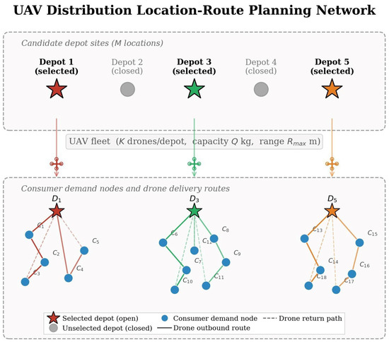
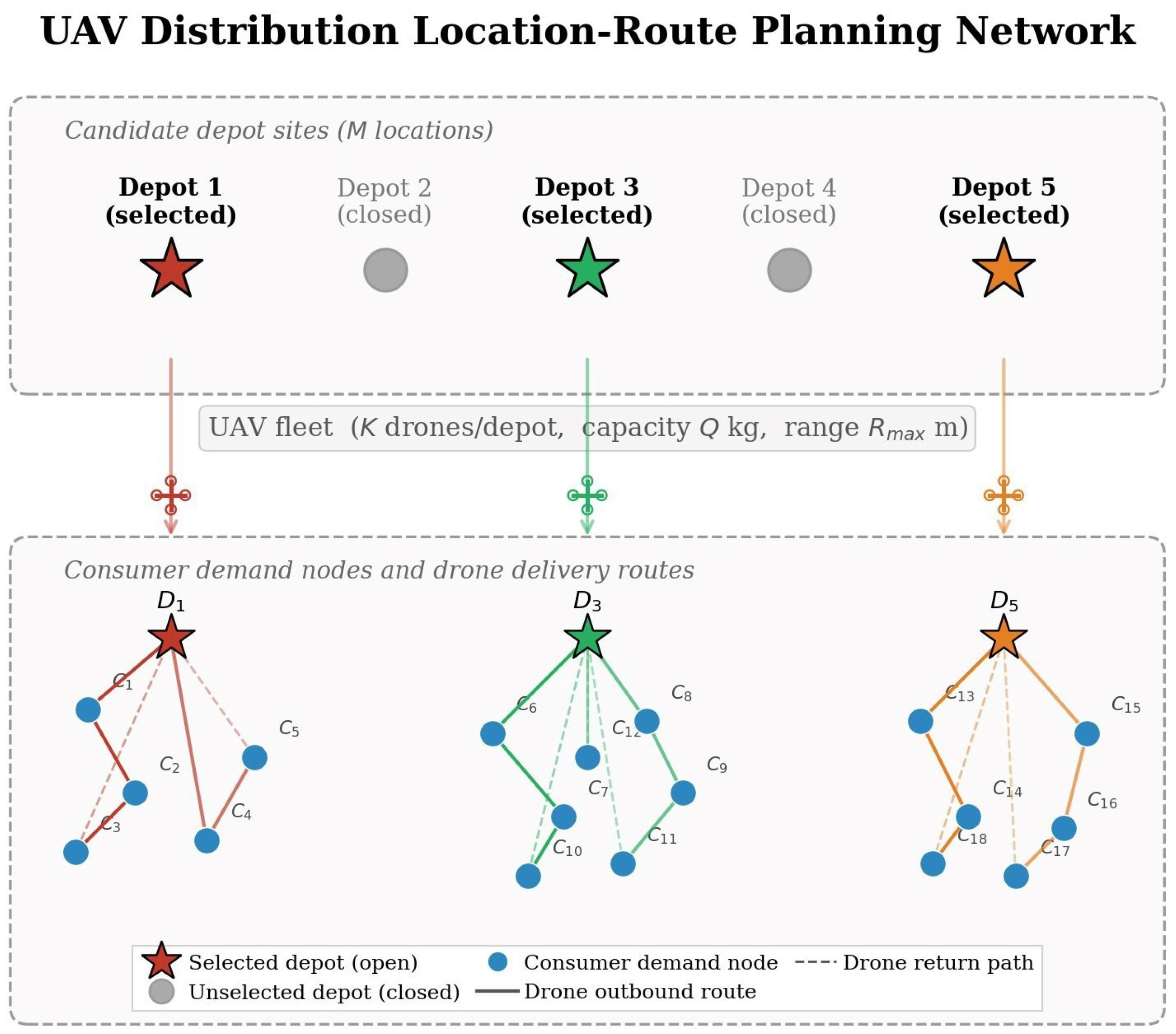
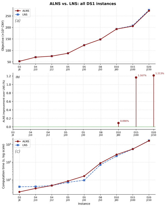
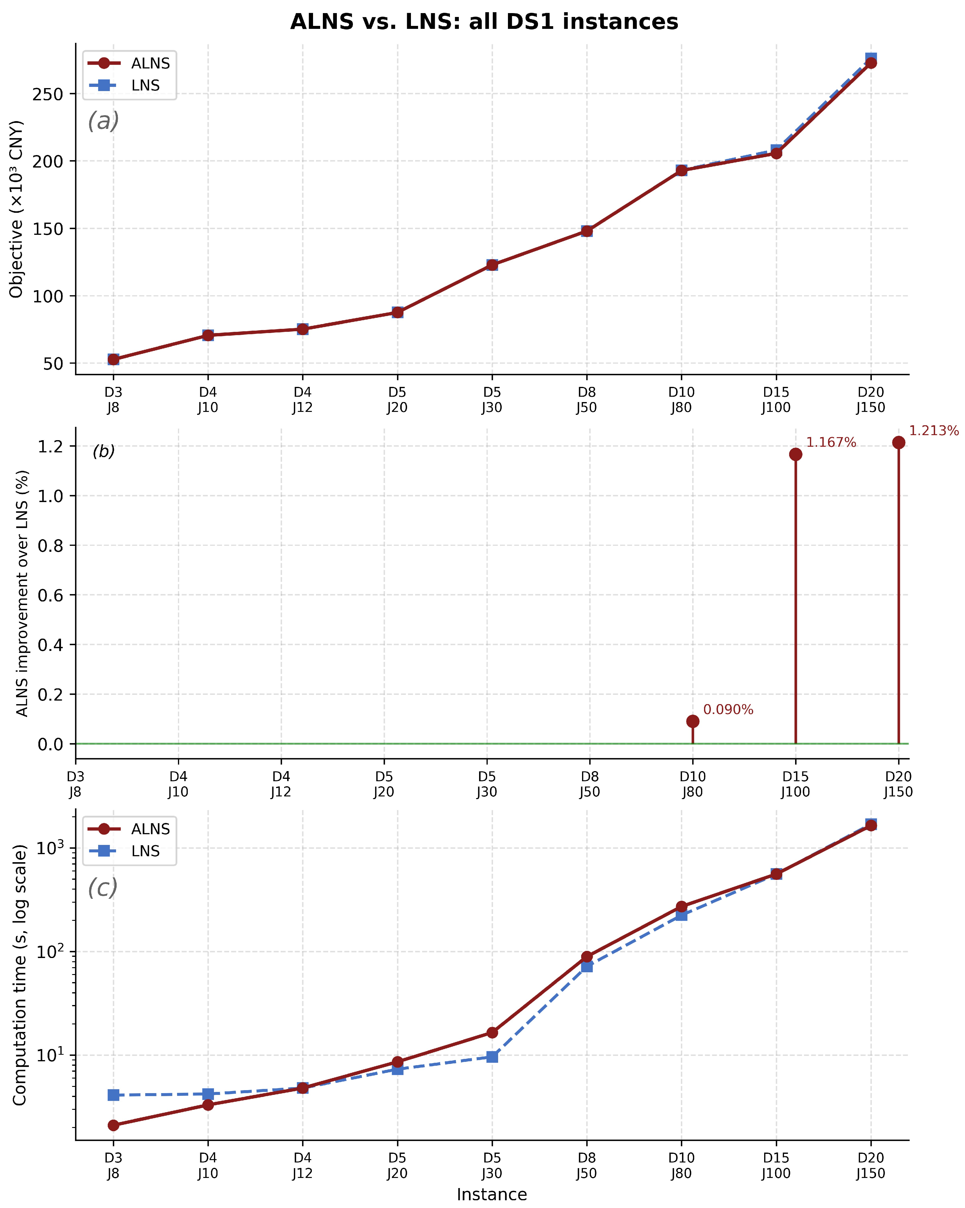
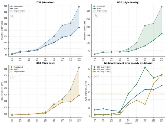
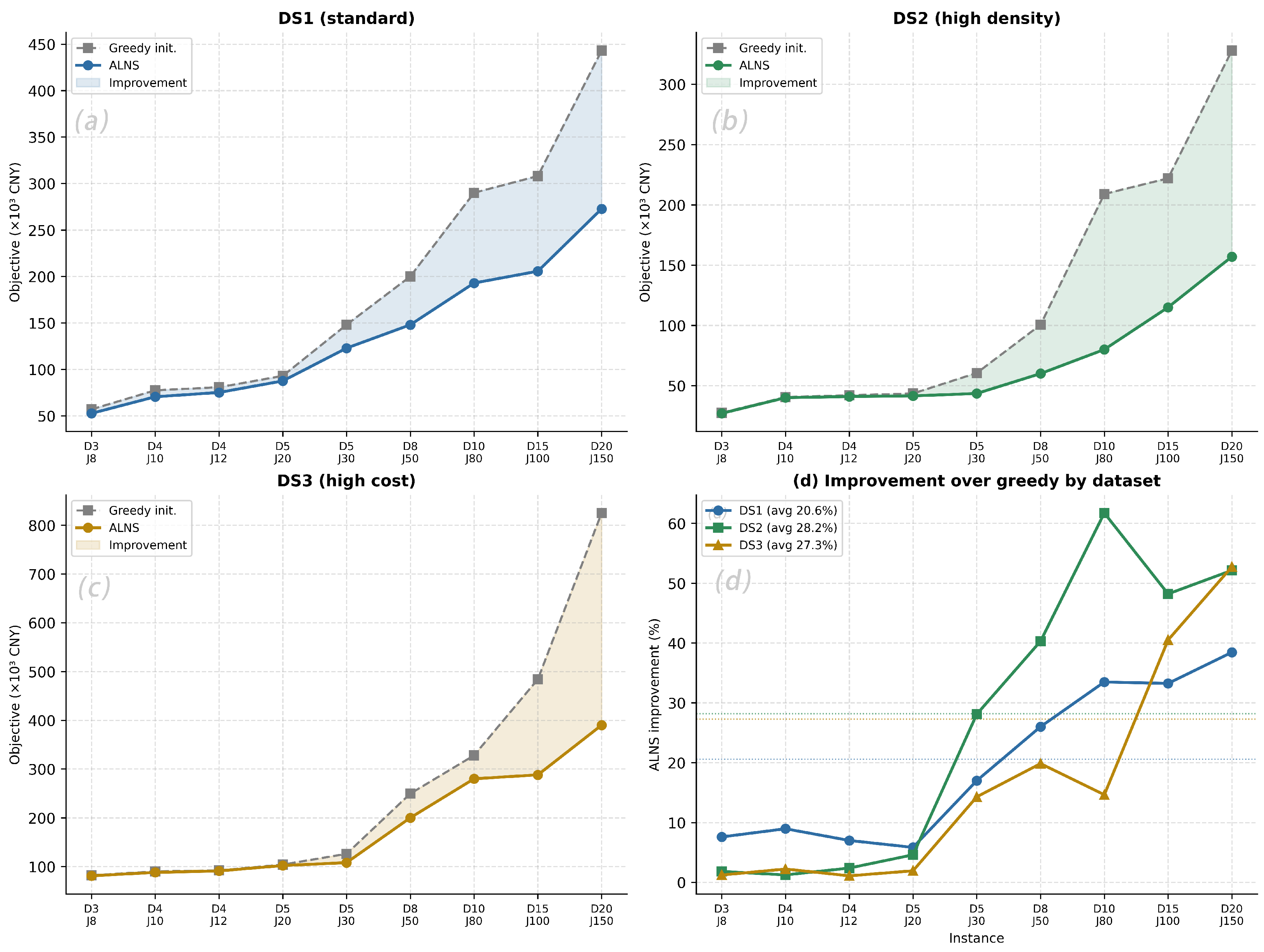
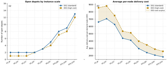
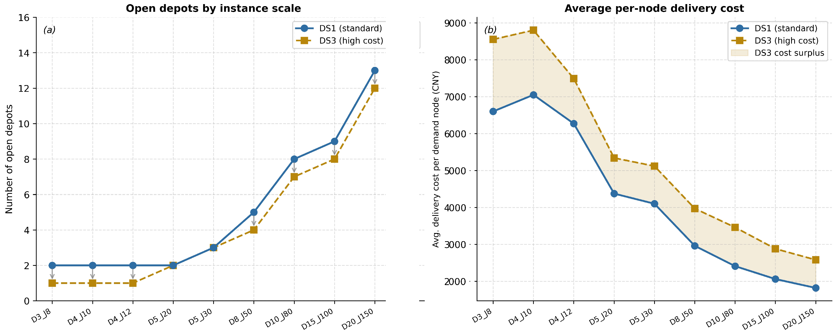
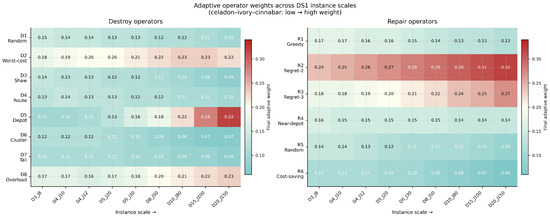
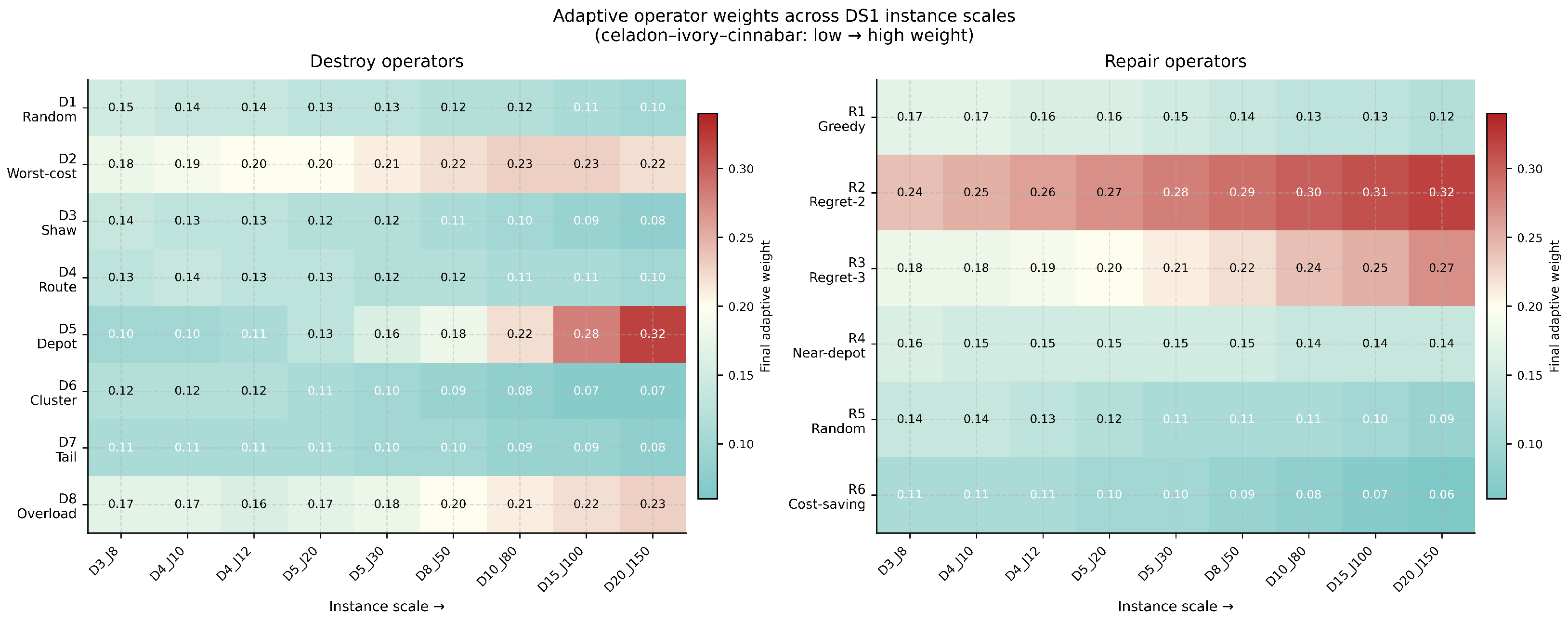
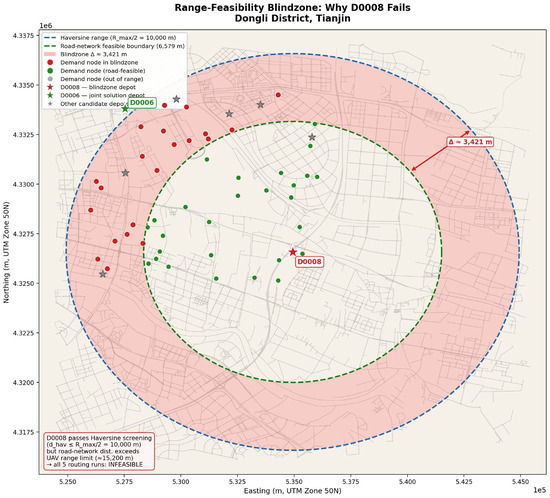
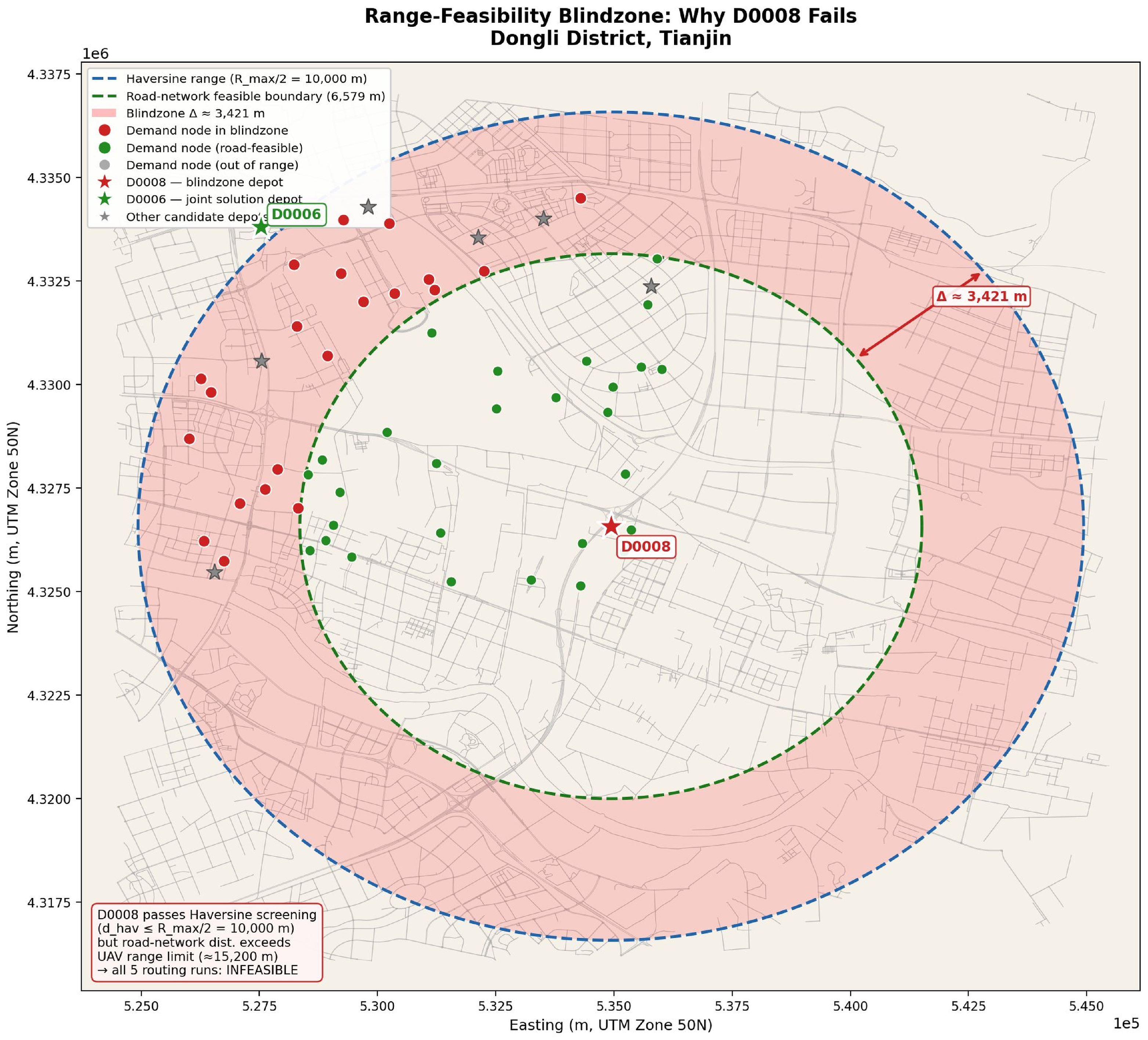
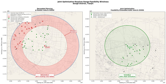
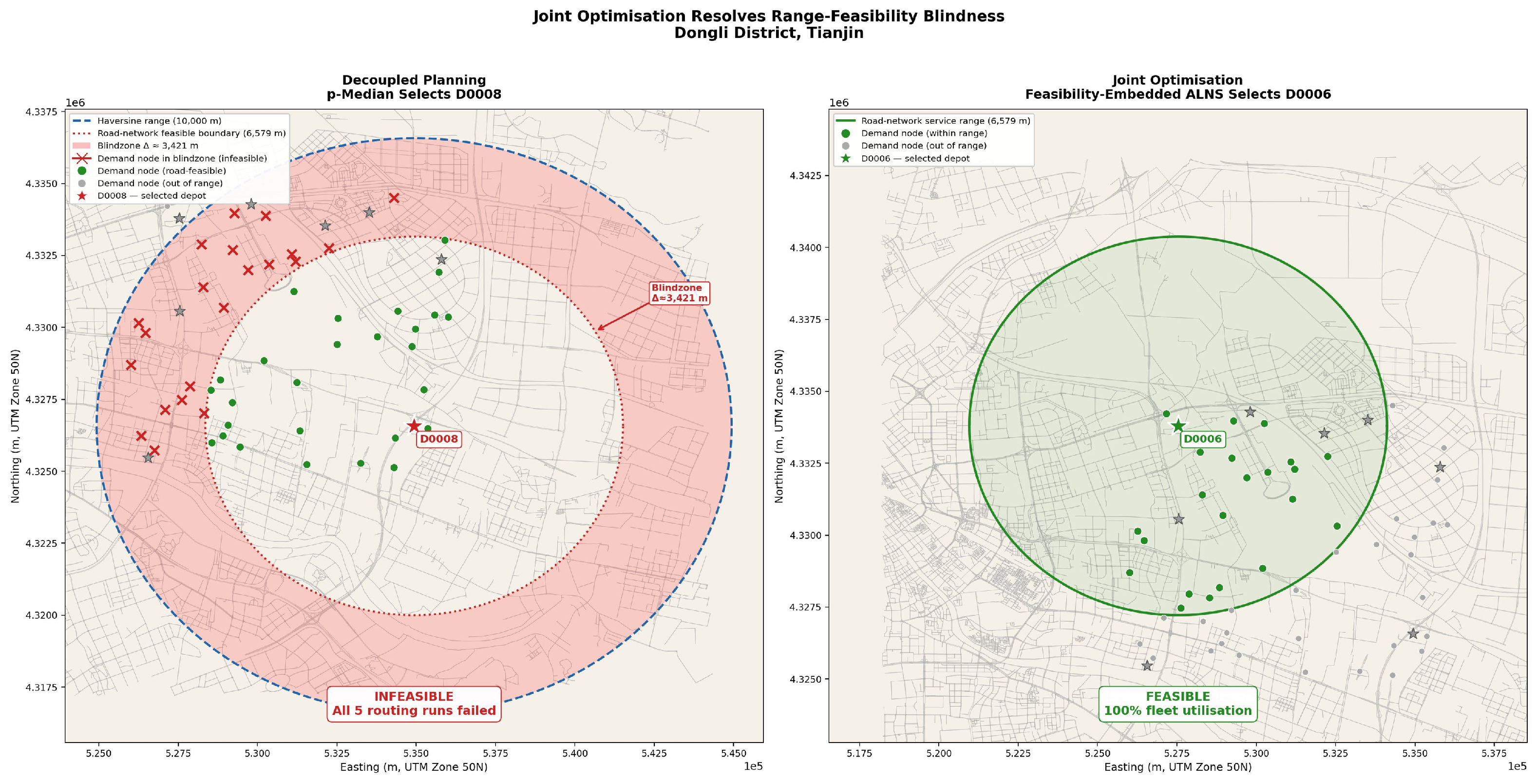
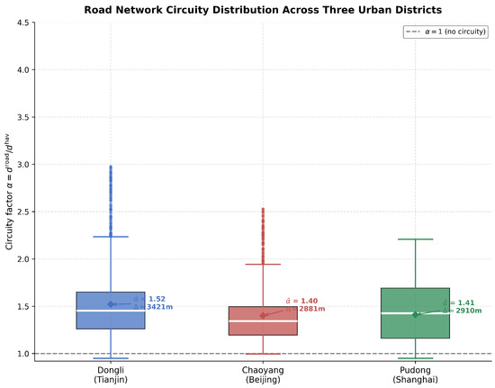
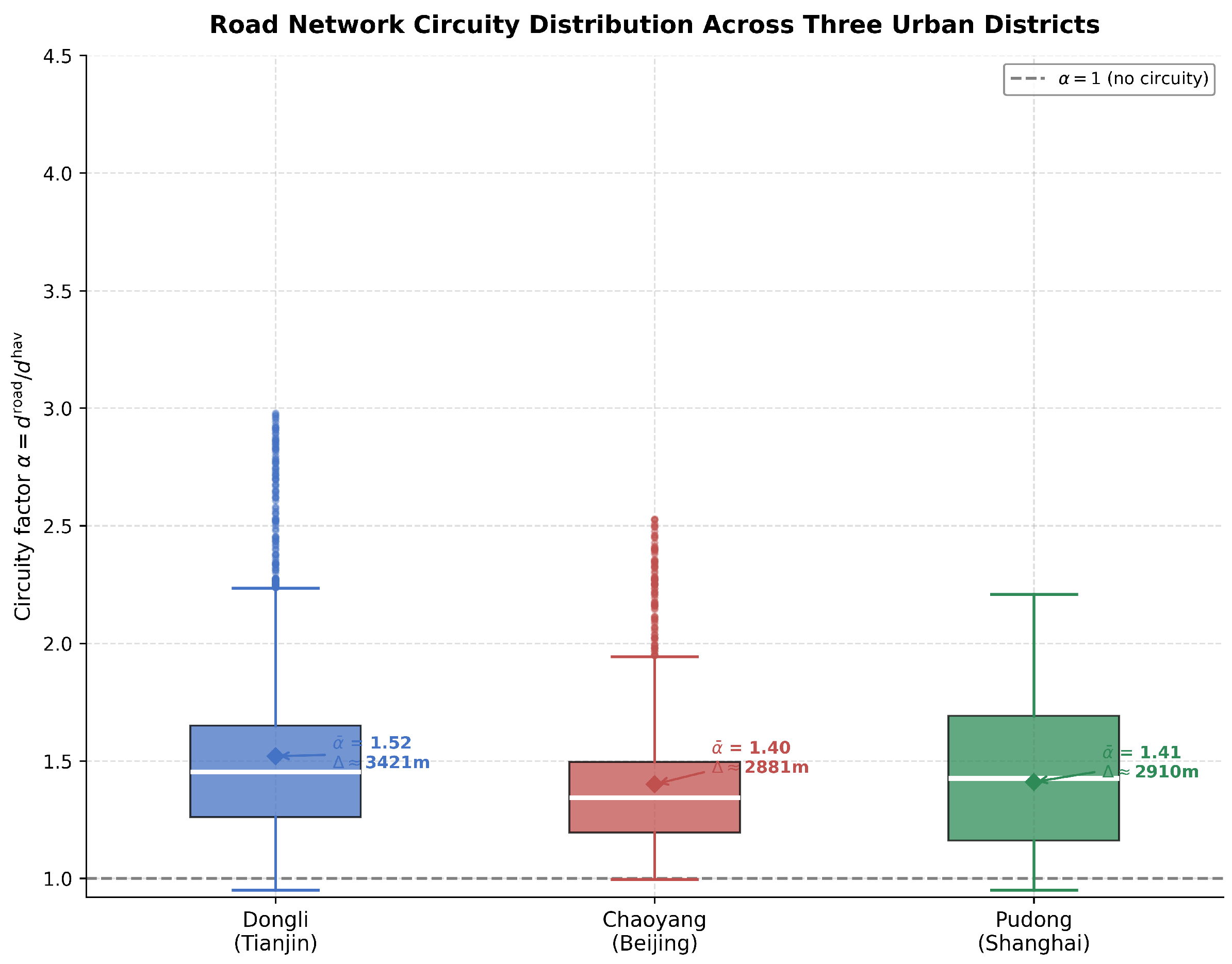

Disclaimer/Publisher’s Note: The statements, opinions and data contained in all publications are solely those of the individual author(s) and contributor(s) and not of MDPI and/or the editor(s). MDPI and/or the editor(s) disclaim responsibility for any injury to people or property resulting from any ideas, methods, instructions or products referred to in the content. |
© 2026 by the authors. Licensee MDPI, Basel, Switzerland. This article is an open access article distributed under the terms and conditions of the Creative Commons Attribution (CC BY) license.