TRACER: A Robust and Autonomous Framework for Angles-Only Orbit Determination

Abstract

Orbit determination from optical observations remains a challenging problem due to the absence of direct range measurements and the presence of sparse, noisy, and irregularly sampled data. This work presents TRACER (Tracking, Recognition, and Analysis for Celestial Ephemerides Retrieval), a robust and fully automated framework for angles-only orbit determination. The proposed approach integrates probabilistic and deterministic strategies within a unified, decision-driven architecture. In particular, statistical ranging is employed for short-arc regimes to explore admissible solutions, while deterministic methods, including modified Gauss and Väisälä techniques, are used for longer arcs and refinement. Candidate solutions are evaluated through a unified scoring function that combines observational consistency with physically motivated penalties. A key contribution of TRACER is the introduction of a randomized subset-selection outer loop, which repeatedly solves the orbit determination problem on different observation subsets and validates solutions against the full dataset, enhancing robustness in challenging scenarios. Additional mechanisms for adaptive subarc selection, recovery from failure, and progressive data assimilation further improve reliability. The resulting framework enables fully autonomous orbit determination without manual intervention, bridging the gap between individual algorithms and operational pipelines for real-world astrometric data processing.

1. Introduction

Orbit determination (OD) is a fundamental capability in astrodynamics, enabling the estimation of the state of a space object from observational data. Accurate knowledge of an object’s orbit is essential for a wide range of applications, including space situational awareness, conjunction assessment, mission design, and on-orbit operations. In recent years, the increasing number of resident space objects has significantly amplified the demand for reliable and automated orbit determination techniques. Ground-based optical observations, in particular, play a key role in tracking objects in Earth orbit and beyond, offering a cost-effective and widely accessible sensing modality.

Astrometric observations from optical telescopes provide only angular measurements (right ascension and declination) without range information, making orbit determination inherently challenging [1]. Also, in real-world survey and follow-up campaigns, observations are often sparse, noisy, and irregularly spaced, frequently limited to short tracklets separated by large temporal gaps, leading to an ill-conditioned problem that may admit multiple feasible solutions, especially for short arcs [2].

Classical approaches to orbit determination are typically divided into two stages: an initial orbit determination (IOD) phase, followed by a refinement step. The IOD phase aims to construct a preliminary estimate of the orbital state from a limited set of observations without requiring an initial guess. Following the IOD estimate, differential correction techniques are employed to refine the orbit by minimizing the residuals between observed and predicted measurements. Batch least squares remains the most widely used approach, providing a statistically grounded framework for incorporating measurement uncertainties [3].

Among the earliest and most widely used IOD methods are those developed by Gauss and Laplace, which exploit geometric relationships between observations to recover the orbit from angles-only measurements [4]. More recent contributions include Gooding’s method [1], which solves the IOD problem iteratively using a Newton-type scheme combined with a Lambert solver, providing improved robustness and precision compared to classical methods.

Several recent works have sought to improve or generalize angles-only IOD methods under challenging observational conditions. For example, Zhang et al. [5] addressed the ill-conditioning of Gooding’s method for short arcs by incorporating multiple observations in a regularized least-squares formulation and refining range initialization through search strategies. Other approaches have pursued alternative formulations of the angles-only IOD problem. Mancini et al. [6] proposed a geometric solution, enabling the recovery of Keplerian conics without requiring an initial guess or numerical propagation, although the method remains sensitive to the geometry of the observed lines of sight. For cislunar and other strongly perturbed regimes, Heidrich and Holzinger [7] introduced a sparse-grid collocation approach, improving robustness over long observation gaps and non-Keplerian dynamics. These contributions improve specific aspects of the IOD step itself, whereas the present work addresses a complementary problem: how OD techniques can be embedded within an autonomous methodology that incorporates practical decision-making and recovery mechanisms for robust processing of real astrometric data.

The difficulty of angles-only IOD is especially pronounced for short arcs, where the absence of range measurements produces large uncertainty along the line of sight, as shown in recent error-analysis studies [8]. This anisotropy reflects the weak observability of the range component: multiple orbit solutions may produce nearly indistinguishable angular residuals over a short arc while corresponding to substantially different positions along the line of sight. Consequently, robust OD frameworks must be able to explore and evaluate multiple plausible candidate solutions and reject poorly conditioned estimates, motivating the candidate-generation, scoring, and recovery mechanisms adopted in the present framework.

To address these limitations, probabilistic approaches such as statistical ranging have been developed [9]. In the original formulation, random realizations of the angular observations are generated according to their uncertainty, while the unknown topocentric ranges at two epochs are sampled, allowing each realization to define a trial orbit. By repeating this process in a Monte Carlo framework, an ensemble of orbits is obtained that approximates the posterior probability distribution of the orbital elements. These methods are particularly effective for short-arc and angles-only data, where multiple orbital solutions may be compatible with the measurements. However, despite efforts to optimize the sampling strategy via Markov Chain Monte Carlo (MCMC) techniques [10] or random walks [11], the reliance on random sampling can lead to significant computational cost and inefficiencies. In this respect, systematic ranging methods, which attempt to mitigate this issue by discretizing the range space and evaluating candidate orbits on a structured grid [12,13], have been proposed, but they still require careful discretization choices and can still be computationally expensive when high resolution is needed.

To address the computational inefficiencies and lack of structure associated with ranging methods, researchers introduced the concept of the Admissible Region (AR). The AR framework characterizes the set of all physically plausible orbits consistent with a collection of angular observations and their instantaneous rates, represented by a 4D vector known as an attributable [14]. Within this formulation, the unknown topocentric range and range-rate are treated as free parameters, and physically motivated constraints are imposed to restrict the solution space to a compact region in the space of these variables. This region can then be systematically sampled, with each sampled point corresponding to a feasible orbit consistent with both the observations and the imposed physical constraints. However, the method’s performance relies on the selection of appropriate physical constraints and, while the AR approach efficiently bounds the set of feasible solutions, it does not inherently provide a probabilistic characterization of uncertainty, often requiring additional modeling or sampling steps when probabilistic information is needed. While probabilistic extensions of this framework, such as Gaussian Mixture Models (GMMs), have been proposed to provide a more explicit representation of uncertainty [15], they often introduce significant computational overhead and remain sensitive to the initial selection of physical constraints.

In the present work, statistical ranging is adopted as one component of the proposed framework because of its ability to represent the ambiguity inherent to short-arc angles-only observations. However, rather than relying on statistical ranging as a standalone solution strategy, it is embedded within a broader decision-driven OD architecture. In particular, the implementation incorporates structured sampling, physical admissibility checks, candidate scoring, and lightweight refinement to improve the efficiency and reliability of the generated solutions. When the statistical-ranging branch does not yield a sufficiently reliable estimate, the framework automatically transitions to deterministic IOD and refinement strategies. Thus, the proposed approach leverages the strengths of probabilistic candidate generation while mitigating its limitations through method selection, solution evaluation, and recovery mechanisms.

Machine learning (ML) approaches have also been explored for orbit determination, particularly for initial orbit estimation and error correction. Early work by Furfaro et al. [16] employed Extreme Learning Machines (ELMs) to learn an inverse mapping from angles-only measurements to orbital state parameters, demonstrating fast training and the ability to approximate nonlinear relationships between observations and states. Peng and Bai [17] proposed a supervised learning framework based on support vector machines (SVMs) to model and correct orbit prediction errors using historical data, showing that learning-based corrections can significantly enhance the accuracy of physics-based predictions. Building on this idea, Peng and Bai [18] investigated artificial neural networks (ANNs) trained on simulated catalog data to improve orbit prediction accuracy, highlighting their capability to approximate complex error dynamics and generalize across future epochs and different resident space objects. More recently, Zhang et al. [19] proposed a neural-network-based approach for improving angles-only orbit determination near Earth–Moon libration orbits by identifying inaccurate angular measurements and re-running the least-squares estimation process with modified observations. Gong et al. [20] developed a deep neural network (DNN) architecture to directly map angles-only measurements to relative orbital states, leveraging nonlinear function approximation to address observability challenges inherent to angles-only orbit determination. Despite these promising results, ML-based approaches rely heavily on the availability of large, high-fidelity, and representative training datasets (often generated from simulations) and their performance may degrade when applied to scenarios that differ from the training distribution, particularly in the presence of model mismatch, unmodeled dynamics, or changing observation conditions.

A more recent development in this area is the use of physics-informed neural networks (PINNs) for orbit determination. Compared to traditional machine learning methods, PINNs incorporate physical constraints directly into the training process, allowing them to learn from data while enforcing consistency with the underlying dynamics [21]. The physics-informed orbit determination (PIOD) framework builds upon this idea by embedding the equations of motion into the loss function and leveraging the theory of functional connections together with an ELM architecture to enable efficient training and improved convergence properties [22,23,24]. Related efforts have explored similar physics-informed formulations for IOD from too-short arcs, where neural networks are used to reconstruct dynamically consistent trajectories starting from coarse estimates [25,26]. While PIOD has shown promise in several test cases, it still requires careful tuning of loss components and neural network hyperparameters, and it does not explicitly account for measurement noise in a probabilistic sense, limiting its ability to quantify uncertainty in the estimated state.

Although a wide range of orbit determination methods exists, their practical application to real observational data often reveals important limitations. Individual techniques are typically designed for specific regimes and may fail when applied outside their domain of validity. The transition from theoretical orbit determination to fully autonomous operational pipelines remains a significant hurdle in astrodynamics.

Large-scale optical surveys, such as those dedicated to space debris characterization [27], have long emphasized the necessity of high-cadence, automated processing to manage the sheer volume of resident space objects. Notable successes in this domain include the Moving Object Processing System (MOPS) developed for Pan-STARRS, which demonstrated the feasibility of linking disparate detections into high-confidence orbits at a massive scale [28]. Related efforts have also formulated optical tracklet association itself as an orbit determination problem. For example, Zhao et al. [29] proposed evaluating candidate associations between optical tracklets by solving an angles-only IOD problem and assessing the consistency of the resulting orbit with the available observations. Such approaches demonstrate the importance of OD within automated optical-survey processing even though their primary objective is association or linkage rather than autonomous recovery of a robust orbit solution.

Angles-only measurements have also been widely studied in relative navigation contexts. Recent reviews and methods have addressed the use of line-of-sight measurements for spacecraft relative navigation [30]. For example, Willis and D’Amico [31] proposed a fast polynomial-dynamics method for angles-only relative navigation using relative orbital elements, while Liao and Oguri [32] developed a relative-navigation approach for asteroid exploration based on angles-only measurements between spacecraft. These problems are related to the present work through the common challenge of missing range information, but they differ in estimation setting and operational assumptions. Indeed, relative-navigation methods often involve a chaser spacecraft, recursive estimation, real-time constraints, or relative-state formulations. In contrast, the present work focuses on batch and autonomous OD from ground-based astrometric observations of space objects, where data may be sparse, irregular, and not acquired under geometries designed for optimal observability.

Taken together, recent work in angles-only OD has produced important advances in individual components of the estimation problem. However, fewer works have addressed the complementary problem of developing an autonomous OD methodology that systematizes practical decision-making, failure recovery, and candidate validation for robust processing of heterogeneous real astrometric data. This methodological gap motivates the present work.

This paper presents a robust and automated orbit determination framework designed to process angles-only observations under a wide range of observational conditions. The proposed approach integrates multiple initial orbit determination strategies, including statistical ranging, Gauss’ method, and Väisälä-type techniques, within a unified decision-driven architecture. Rather than relying on a single estimation method, the framework adaptively selects and combines complementary techniques based on the characteristics of the available observations, such as arc length and data quality.

The present work has two closely related objectives. First, it provides a structured and formal treatment of a robust orbit-determination pipeline that has been implemented and extensively used within the publicly available Find_Orb software (https://www.projectpluto.com/find_orb.htm, accessed on 29 April 2026), but whose underlying methodologies, heuristics, and recovery strategies have not previously been systematically formalized and analyzed in the scientific literature. While these techniques build upon established orbit-determination principles, several components correspond to practical methodological extensions and operational refinements that have evolved through extensive real-world application over many years.

Second, this work introduces TRACER (Tracking, Recognition, and Analysis for Celestial Ephemerides Retrieval), an autonomous angles-only orbit-determination methodology built around this estimation architecture. In particular, TRACER extends the original methodology through the introduction of a randomized subset-selection outer loop in which orbit determination is repeatedly performed on randomly selected subsets of observations and the resulting candidate solutions are subsequently validated against the full dataset. This strategy significantly improves robustness in challenging scenarios where direct estimation from the complete observation arc may fail due to unfavorable geometry, sparse observations, or inconsistent measurements. The resulting system promotes a high degree of autonomy in orbit determination, reducing the need for manual intervention while mitigating common failure modes associated with classical approaches.

Therefore, while the proposed approach does not seek to replace classical initial orbit-determination or estimation methods with an entirely new theoretical formulation, the contribution of this work extends beyond software implementation or algorithmic orchestration alone. In particular, the present work formalizes and analyzes advanced operational methodologies that have remained largely embedded within source code and expert practice despite extensive practical use, while also introducing new autonomous recovery strategies for challenging angles-only orbit-determination scenarios.

The main contributions of this work can be summarized as follows:

• A structured and formal analysis of advanced orbit-determination procedures, heuristics, and recovery mechanisms that have evolved within the operational use of Find_Orb but have not previously been systematically formalized and analyzed in the scientific literature.
• The formulation of an autonomous angles-only orbit-determination methodology that unifies statistical ranging, deterministic IOD, adaptive refinement, and decision-driven recovery strategies within a single estimation framework.
• The introduction of a randomized subset-selection and full-dataset validation strategy that improves robustness in challenging scenarios characterized by sparse observations, unfavorable geometry, or data inconsistencies.
• The demonstration of autonomous orbit recovery capabilities on real astrometric datasets collected from ground-based optical sensors across diverse observational regimes.

This paper is organized as follows. Section 2 introduces the orbit determination problem formulation and provides an overview of the hierarchical architecture of the proposed framework. Section 3 describes the inner orbit-determination pipeline, including the statistical ranging, deterministic IOD, refinement, recovery, and solution-evaluation procedures. Section 4 presents TRACER’s outer-loop framework based on randomized subset selection and full-dataset validation. Section 5 presents the results of applying the proposed framework to real astrometric data, demonstrating its performance and robustness across a range of scenarios. Finally, Section 6 summarizes the main contributions of this work and outlines potential directions for future research.

2. Orbit Determination Framework

2.1. Problem Formulation

The objective of the orbit determination process is to estimate the orbital state of a space object from a set of astrometric observations. The available measurements consist of angular data, expressed in terms of right ascension and declination, acquired at discrete time instants by ground-based optical sensors. These observations provide directional information only, without direct knowledge of the range to the object, resulting in an inherently underdetermined estimation problem.

Let $\mathcal{Y}={({\alpha }_i,{\delta }_i,t_i)}_{i=1}^N$ denote the set of observations, where ${\alpha }_i$ and ${\delta }_i$ are the right ascension and declination measured at time $t_i$. The goal is to estimate the corresponding orbital state ${\mathbf{x}}_0$ at a reference epoch $t_0$, such that the predicted observations obtained through orbital propagation and measurement modeling are consistent with $\mathcal{Y}$. This is achieved through a combination of initial orbit determination techniques and subsequent refinement via differential correction.

2.2. Overview of the Proposed Pipeline

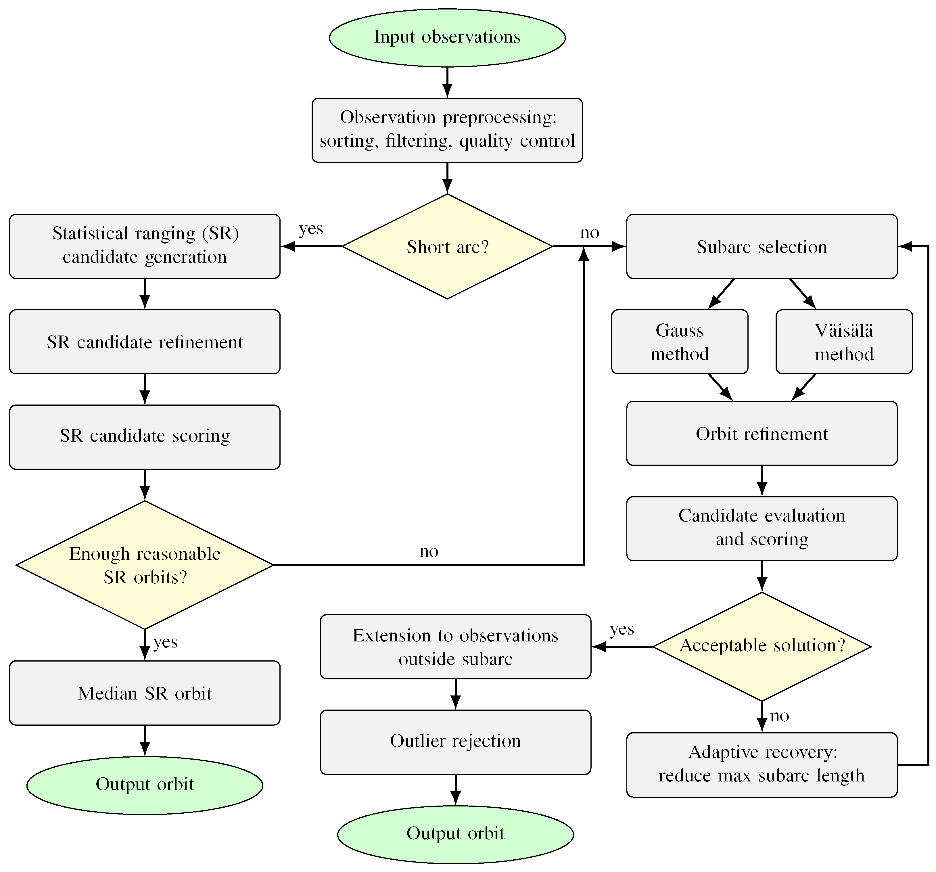
The proposed orbit determination framework is structured as a hierarchical architecture. At the core lies the Find_Orb-inspired orbit determination pipeline, illustrated in Figure 1, which integrates statistical ranging, classical initial orbit determination methods, and refinement procedures.

The core framework consists of a decision-driven sequence of estimation steps, in which different orbit determination techniques are activated depending on the characteristics of the observation set. In particular, the algorithm distinguishes between short-arc and long-arc regimes based on the temporal span of the observations. For short arcs, a probabilistic approach based on statistical ranging is first employed, as it is better suited to handle the inherent ambiguity of limited observational data. If this stage produces a sufficient number of reliable solutions, a representative orbit is extracted and returned. Otherwise, the algorithm reverts to a deterministic orbit determination procedure applied to selected subsets of observations, which also serves as the default strategy for longer arcs.

While the statistical ranging branch directly produces a set of candidate solutions when successful, the deterministic orbit determination branch relies on iterative refinement and evaluation. In both cases, candidate solutions are improved through differential correction procedures and assessed using quantitative scoring metrics. However, the two approaches differ in how these steps are embedded within the estimation process.

In the statistical ranging branch, refinement and scoring are applied in a single pass to an ensemble of independently generated candidates, after which a representative solution is selected if sufficient high-quality orbits are identified. If this condition is not met, the algorithm transitions to the deterministic pipeline.

In contrast, the deterministic branch embeds these operations within an iterative loop, enabling adaptive adjustments of the estimation strategy based on intermediate results, such as modifying the observation subset or refining candidate solutions. Candidate orbits are generated using both Gauss and Väisälä methods, and the final estimate is selected based on their relative scores. This adaptive logic enables the framework to recover from failure cases and improve robustness without requiring manual intervention.

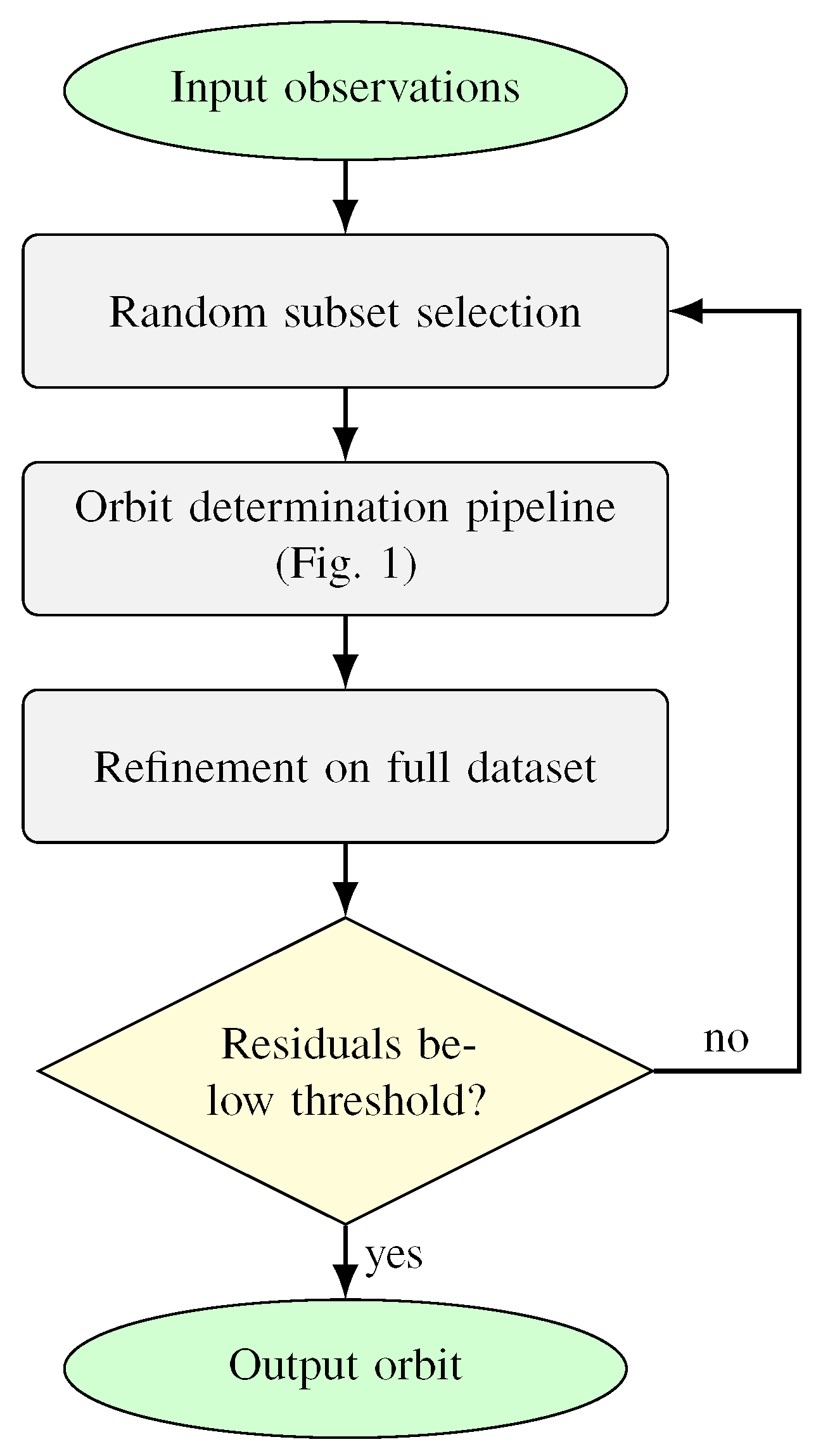
In TRACER, this core pipeline is embedded within an outer iterative loop, illustrated in Figure 2, that performs orbit determination on randomly selected subsets of the observations and validates the resulting solutions against the full dataset. At each iteration, a subset of observations is selected, the inner pipeline is executed, and the resulting solution is refined using all available observations. The solution is accepted only if it satisfies a prescribed residual threshold; otherwise, a new subset is sampled and the process is repeated. This outer-loop strategy significantly enhances robustness by enabling multiple independent attempts at orbit reconstruction under different observational configurations.

It is important to distinguish between the two levels of the proposed architecture. In Section 3, the inner orbit-determination pipeline, largely based on methodologies implemented in Find_Orb, is described in detail. This core pipeline includes scoring and evaluation metrics, statistical ranging, deterministic IOD methods, refinement procedures, and recovery strategies. TRACER builds upon this foundation by embedding the pipeline within an additional autonomous outer-loop framework based on randomized subset selection and full-dataset validation, described in Section 4.

3. Inner Orbit Determination Pipeline

3.1. Solution Scoring and Evaluation

A key component of the proposed framework is a unified scoring function used to evaluate and rank candidate orbit solutions generated by different IOD methods. This score provides a quantitative measure of both observational consistency and physical plausibility, enabling a consistent comparison across heterogeneous solution sets.

3.1.1. Data Fit Term

The primary contribution to the score is given by a weighted root-mean-square (RMS) of the residuals between observed and predicted measurements.

The residuals are first computed in right ascension and declination as

$$\Delta {\alpha }_i=({\alpha }_i-{\alpha }_i^{\mathrm{comp}})\cos {\delta }_i,\Delta {\delta }_i={\delta }_i-{\delta }_i^{\mathrm{comp}}$$

(1)

which define a local tangent-plane representation of the angular residuals.

For reference, a baseline metric is given by the unweighted RMS of the angular residuals,

$${\mathrm{RMS}}_{\mathrm{unw}}=\sqrt{{\displaystyle \frac{1}{N}}\sum _{i=1}^N\left(\Delta {\alpha }_i^2+\Delta {\delta }_i^2\right)}$$

(2)

which provides a direct geometric measure of the residual magnitude in the tangent plane.

However, this formulation does not account for anisotropic uncertainties arising from astrometric and timing errors. To address this, the residuals are grouped into a vector ${\mathsf{ϵ}}_i=(\Delta {\alpha }_i,\Delta {\delta }_i)$ and then projected onto a local reference frame aligned with the apparent motion direction ${\mathit{v}}_{\mathrm{app},i}=({\dot{\alpha }}_i,{\dot{\delta }}_i)$, yielding the along-track and cross-track components

$${ϵ}_{\Vert ,i}={\widehat{\mathit{t}}}_i·{\mathsf{ϵ}}_i,{ϵ}_{\perp ,i}={\widehat{\mathit{n}}}_i·{\mathsf{ϵ}}_i,$$

(3)

where ${\widehat{\mathit{t}}}_i={\mathit{v}}_{\mathrm{app},i}/∥{\mathit{v}}_{\mathrm{app},i}∥$ and ${\widehat{\mathit{n}}}_i$ are unit vectors parallel and orthogonal to the apparent motion, respectively.

The residuals are scaled by their respective standard deviations ${\sigma }_{\Vert }$ and ${\sigma }_{\perp }$, leading to a weighted RMS defined as

$${\mathrm{RMS}}_{\mathrm{w}}=\sqrt{{\displaystyle \frac{1}{N}}\sum _{i=1}^N\left[{\left({\displaystyle \frac{{ϵ}_{\Vert ,i}}{{\sigma }_{\Vert ,i}}}\right)}^2+{\left({\displaystyle \frac{{ϵ}_{\perp ,i}}{{\sigma }_{\perp ,i}}}\right)}^2\right]}$$

(4)

where N is the number of observations. The cross-track uncertainty is given by the astrometric measurement uncertainty (i.e., the error in the angular position),

$${\sigma }_{\perp }={\sigma }_{\mathrm{astro}}$$

(5)

while the along-track uncertainty additionally accounts for timing errors, which project along the direction of apparent motion,

$${\sigma }_{\Vert }=\sqrt{{\sigma }_{\mathrm{astro}}^2+{\left(v_{\mathrm{app}}{\sigma }_t\right)}^2}$$

(6)

where ${\sigma }_t$ is the timing uncertainty. This results in an anisotropic error model, with increased uncertainty along the direction of motion.

The data fit contribution to the score is then defined as

$$S_{\mathrm{fit}}={\displaystyle \frac{1}{2}}{\mathrm{RMS}}_{\mathrm{w}}·w\left(N\right),$$

(7)

where $w\left(N\right)$ is a scaling factor that reduces the weight of solutions obtained from limited observational data. In this work, arcs with fewer than $N_{\min }=6$ observations are down-weighted according to

$$w\left(N\right)=\left\{\begin{array}{cc}{\displaystyle \frac{N-2}{N_{\min }-2}}\hfill & \mathrm{if}N<N_{\min }\hfill \\ 1\hfill & \mathrm{otherwise}\hfill \end{array}\right.$$

(8)

3.1.2. Physical Plausibility Penalties

To complement the data fit term, the scoring function includes penalty terms designed to discourage physically unlikely orbital configurations. These penalties are derived from the orbital elements associated with each candidate solution.

An additional penalty is applied to elliptical orbits whose periapsis distance $r_p=a(1-e)$ lies below the radius R of the central body. These impacting trajectories are penalized according to

$$S_{\mathrm{imp}}=\left\{\begin{array}{cc}{C}_{\mathrm{imp}}\hfill & \mathrm{if}e<1\mathrm{and}{r}_p<R\hfill \\ 0\hfill & \mathrm{otherwise}\hfill \end{array}\right.$$

(9)

where $C_{\mathrm{imp}}={10}^4$. This term discourages physically infeasible trajectories that intersect the central body.

For heliocentric orbits only, a penalty is applied based on the eccentricity e and inclination i. The heliocentric penalty term is defined as

$$S_{\mathrm{helio}}=S_e+S_{\mathrm{hyp}}+S_{\mathrm{inc}}+S_{\mathrm{emp}}$$

(10)

The first term, $S_e$, is defined as

$$S_e={\displaystyle \frac{e}{2}}$$

(11)

This introduces a mild regularization effect, biasing the solution toward bounded, low-eccentricity orbits in cases where the observational residuals alone do not strongly discriminate between candidates.

The second term, $S_{\mathrm{hyp}}$, is defined as

$$S_{\mathrm{hyp}}=\left\{\begin{array}{cc}{C}_{\mathrm{hyp}}(e-1.01)\hfill & \mathrm{if}e>1.01\hfill \\ 0\hfill & \mathrm{otherwise}\hfill \end{array}\right.$$

(12)

where $C_{\mathrm{hyp}}={10}^3$. $S_{\mathrm{hyp}}$ strongly penalizes hyperbolic solutions, effectively suppressing unbound heliocentric trajectories.

The third term, $S_{\mathrm{inc}}$, weakly penalizes high-inclination heliocentric orbits, particularly those with moderate eccentricity, as they are less commonly observed in typical populations. This term is defined as

$$S_{\mathrm{inc}}=\left\{\begin{array}{cc}\min \left(0.2,0.2(i-0.5)\right)·\varphi \left(e\right)\hfill & \mathrm{if}i>0.5\mathrm{and}e<0.8\hfill \\ 0\hfill & \mathrm{otherwise}\hfill \end{array}\right.$$

(13)

where i is the heliocentric inclination in radians, and

$$\varphi \left(e\right)=\left\{\begin{array}{cc}1\hfill & \mathrm{if}e\le 0.6\hfill \\ {\displaystyle \frac{0.8-e}{0.2}}\hfill & \mathrm{if}0.6<e<0.8\hfill \end{array}\right.$$

(14)

This term introduces a mild bias against high-inclination, low-eccentricity solutions, while allowing highly eccentric (comet-like) orbits to remain largely unpenalized.

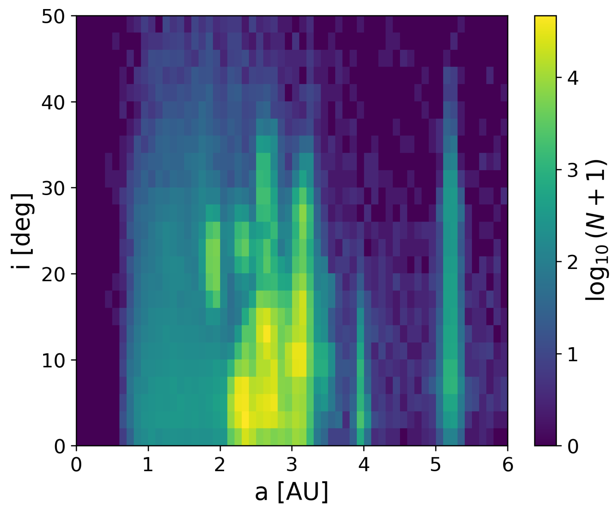
The fourth term, $S_{\mathrm{emp}}$, is an empirical correction based on the observed distribution of orbital elements in real populations. In particular, it is derived from the joint distribution of semimajor axis and inclination obtained from the Minor Planet Center (MPC) database [33], shown in Figure 3. This term is introduced only as a weak regularization term for cases in which multiple candidate solutions provide comparable observational residuals. Its purpose is not to impose a probabilistic prior or to force the solution toward the most common asteroid populations, but rather to provide a mild tie-breaking preference against dynamically unusual solutions when the data fit alone is insufficiently discriminative. The magnitude of this correction is kept small relative to the dominant residual-based contribution and to the stronger feasibility penalties used to reject clearly non-physical solutions. Consequently, a candidate orbit with sufficiently better observational consistency can still be selected even if it corresponds to a rare or atypical orbital configuration.

3.1.3. Total Score

The final score assigned to a candidate orbit is obtained by combining the data fit term and the penalty contributions,

$$S=S_{\mathrm{fit}}+S_{\mathrm{pen}}$$

(15)

where $S_{\mathrm{pen}}=S_{\mathrm{imp}}+S_{\mathrm{helio}}$ aggregates the physical plausibility terms described above.

The penalty terms are intended to complement, rather than replace, the observational residuals. Their main role is to discriminate among candidate solutions when the available angular data alone are insufficient to clearly identify a unique orbit, and to prevent early-stage selection of physically implausible trajectories that could lead the subsequent refinement process toward poor local solutions. For this reason, the penalties are designed as coarse regularization terms and feasibility filters, not as finely tuned parameters that determine the final estimate.

In the proposed framework, the final orbit is obtained only after candidate refinement and residual-based evaluation against the available observations. Thus, while the penalty terms improve robustness during candidate ranking and rejection, the accepted solution remains primarily driven by observational consistency. This reduces the sensitivity of the final result to the precise numerical values or specific analytical forms of the individual penalty terms, provided that they preserve their intended qualitative role: strongly rejecting clearly infeasible solutions and weakly regularizing ambiguous but otherwise plausible candidates.

3.2. Short-Arc Regime: Statistical Ranging

3.2.1. Overview

In the case of optical observations, each measurement provides only angular information, defining a line of sight from the observer to the object. The corresponding range, i.e., the distance along this line of sight, remains unknown. As a result, for short observation arcs, the orbit determination problem is inherently underconstrained and admits a continuum of possible solutions.

Statistical ranging addresses this ambiguity by sampling the unknown range parameters at selected observation epochs. In particular, candidate orbits are generated by assigning plausible values to the ranges associated with two observations, which, together with the corresponding line-of-sight directions and observation times, allow for the reconstruction of a full state vector. By repeating this process over a large number of samples, a set of admissible orbital solutions consistent with the observations is obtained.

In the present implementation, rather than sampling the ranges at both endpoints of the observation arc, a slightly different parameterization is adopted. The topocentric distance is sampled at one endpoint of the arc (taken as the initial observation), while the geometry at the opposite endpoint is characterized through a second scalar parameter.

3.2.2. Admissible Range for the First Observation

A lower bound on the sampled topocentric distance ${\rho }_1$ is introduced to avoid degenerate or non-physical configurations. This bound is defined as

$${\rho }_{1,\min }(\Delta t)=\max \left[{\rho }_{\mathrm{GEO}}{\left({\displaystyle \frac{3\Delta t}{T_{\mathrm{GEO}}}}\right)}^{2/3},v_{\min }\Delta t\right]$$

(16)

where $\Delta t$ is the time span between the two selected observations, ${\rho }_{\mathrm{GEO}}$ and $T_{\mathrm{GEO}}$ are the geostationary orbital radius and period, respectively, and $v_{\min }=1\mathrm{km}/\mathrm{s}$.

The first term in Equation (16) follows from Kepler’s third law by scaling the geostationary orbital radius under the requirement that the orbital period satisfies $T\gtrsim 3\Delta t$. This condition prevents the inclusion of fast, tightly bound orbits that would produce excessive curvature over the observation arc and are therefore inconsistent with short-arc measurements.

The second term in Equation (16) enforces a minimum traveled distance over the observation interval. This condition excludes solutions corresponding to unrealistically small object–observer distances combined with negligible motion, which would otherwise satisfy the angular observations but lead to physically implausible or numerically unstable configurations. The value $v_{\min }=1\mathrm{km}/\mathrm{s}$ is chosen as a conservative lower bound on typical orbital velocities, ensuring that feasible orbital solutions are retained while near-static or degenerate configurations are discarded.

The upper admissible range ${\rho }_{1,\max }$ is not prescribed a priori, but is instead determined by enforcing dynamical consistency between the sampled distance and the observed geometry. Let ${\mathbf{q}}_1,{\mathbf{q}}_2$ denote the observer positions at the two epochs, and ${\mathbf{u}}_1,{\mathbf{u}}_2$ the corresponding line-of-sight unit vectors. For a sampled distance ${\rho }_1$, the object position at the first observation is

$${\mathbf{r}}_1={\mathbf{q}}_1+{\rho }_1{\mathbf{u}}_1$$

(17)

Defining

$$\mathbf{a}={\mathbf{q}}_1-{\mathbf{q}}_2-{\mathbf{u}}_2\left({\mathbf{u}}_2·({\mathbf{q}}_1-{\mathbf{q}}_2)\right),\mathbf{b}={\mathbf{u}}_1-{\mathbf{u}}_2({\mathbf{u}}_2·{\mathbf{u}}_1)$$

(18)

the minimum distance between ${\mathbf{r}}_1$ and the second observation ray is

$$\mathbf{d}\left({\rho }_1\right)=\mathbf{a}+{\rho }_1\mathbf{b}$$

(19)

Admissible values of ${\rho }_1$ are required to satisfy the condition that this distance can be traversed within the time span $\Delta t$ without exceeding the local escape speed, i.e.,

$$\parallel \mathbf{d}\left({\rho }_1\right)\parallel \le v_{\mathrm{esc}}\Delta t,v_{\mathrm{esc}}^2={\displaystyle \frac{2\mu }{\parallel {\mathbf{r}}_1\parallel }}$$

(20)

where $\mu$ is the gravitational parameter of the central body. This condition leads to a sixth-degree polynomial inequality in ${\rho }_1$. The admissible values of ${\rho }_1$ are obtained by retaining only the physically meaningful solutions (i.e., ${\rho }_1\ge 0$) and applying the lower bound constraint (i.e., ${\rho }_1\ge {\rho }_{1,\min }$). The resulting feasible set can be expressed as a union of intervals

$${\rho }_1\in \left(\bigcup _k[{\tilde{\rho }}_{2k-1},{\tilde{\rho }}_{2k}]\right)\cap [{\rho }_{1,\min },\infty )$$

(21)

where $\left\{{\tilde{\rho }}_i\right\}$ denote the real roots of the polynomial, sorted in ascending order. The sampling domain is then constructed from these intervals.

3.2.3. Admissible Geometry at the Second Observation

Once a value of ${\rho }_1$ is sampled, the admissible range for the second observation ${\rho }_2$ is determined by the requirement that the distance between the two positions does not exceed the maximum reachable distance under an escape-speed assumption, i.e.,

$$\parallel {\mathbf{r}}_2-{\mathbf{r}}_1\parallel \le v_{\mathrm{esc}}\Delta t$$

(22)

This condition defines a bounded interval along the second line of sight, corresponding to the intersection between the line ${\mathbf{r}}_2={\mathbf{q}}_2+{\rho }_2{\mathbf{u}}_2$ and the sphere of radius $v_{\mathrm{esc}}\Delta t$ centered at ${\mathbf{r}}_1$. This interval is centered around the point on the second line of sight closest to ${\mathbf{r}}_1$, which corresponds to the orthogonal projection of ${\mathbf{r}}_1$ onto the second line of sight,

$${\rho }_{2,\mathrm{proj}}=({\mathbf{r}}_1-{\mathbf{q}}_2)·{\mathbf{u}}_2$$

(23)

Then, the admissible values of ${\rho }_2$ can be expressed as

$${\rho }_2\in \left[{\rho }_{2,\mathrm{proj}}-\sqrt{d_{\mathrm{esc}}^2-d^2},{\rho }_{2,\mathrm{proj}}+\sqrt{d_{\mathrm{esc}}^2-d^2}\right]$$

(24)

where $d_{\mathrm{esc}}=v_{\mathrm{esc}}\Delta t$.

Rather than sampling ${\rho }_2$ directly, this interval is parameterized using a scalar variable $\beta \in [-1,1]$, such that

$${\rho }_2={\rho }_{2,\mathrm{proj}}+\beta \sqrt{d_{\mathrm{esc}}^2-d^2}$$

(25)

This formulation introduces two independent sampling parameters, $({\rho }_1,\beta )$, which play a role analogous to the classical pair of endpoint ranges $({\rho }_1,{\rho }_2)$. However, the second parameter $\beta$ spans only dynamically admissible configurations, ensuring that the resulting trial orbits are consistent with both the observational geometry and the imposed dynamical constraints.

3.2.4. Sampling Strategy

Unlike purely random Monte Carlo sampling, which may lead to clustering and poor coverage of the admissible region, the proposed approach employs low-discrepancy sequences, specifically Halton sequences, to generate quasi-random samples. In practice, the Halton sequence is used to generate samples in the unit interval $(0,1)$, which are then mapped to physically admissible ranges for ${\rho }_1$ and $\beta$. This ensures a more uniform and efficient exploration of the domain, improving the probability of identifying dynamically consistent solutions.

3.2.5. Remarks on the Choice of the Heuristic Parameters

The statistical ranging procedure described above relies on a small number of heuristic bounds. These parameters are not intended as case-specific tuning constants, but as conservative admissibility filters used to restrict the sampling domain to geometrically and dynamically plausible configurations.

For instance, the first term in the lower bound in Equation (16) prevents the sampler from considering unrealistically close or rapidly curving solutions over short observation arcs, while the second term, $v_{\min }\Delta t$, imposes a minimum displacement scale that removes near-static or numerically degenerate configurations. Analogously, the upper admissible range is determined from the requirement that the displacement between the two endpoint positions be dynamically reachable within the available time span.

Overall, these choices should be interpreted as broad physical filters rather than optimized hyperparameters. The final selection of a candidate orbit is governed by subsequent refinement, scoring, and residual-based validation against the observations, which reduces the dependence of the result on any single heuristic parameter.

3.2.6. Orbit Construction and Refinement

For each sampled pair $({\rho }_1,\beta )$, a trial orbit is constructed by solving a two-point boundary value problem (TPBVP) between ${\mathbf{r}}_1$ and ${\mathbf{r}}_2$, as described in Appendix A. While this construction ensures consistency with the two selected observations, it does not explicitly enforce agreement with the remaining measurements in the observation set. To address this limitation, each candidate orbit is refined through a lightweight differential correction step that incorporates all available observations.

Given a trial orbit, residuals in right ascension and declination are evaluated at all observation epochs. These residuals are approximated using linear models of the form

$$\Delta \alpha \left(t\right)\approx A+Bt,\Delta \delta \left(t\right)\approx C+Dt$$

(26)

where the coefficients A, B, C, and D are obtained via least-squares fitting.

The endpoint observations are then corrected by subtracting the corresponding residual trends, and a new orbit is reconstructed using the corrected endpoint states. In this way, the refinement step effectively incorporates information from the full observation arc while preserving the underlying two-point structure of the solution.

The constant terms A and C capture systematic offsets in right ascension and declination, while the linear terms B and D represent temporal trends in the residuals. Removing these components reduces the dominant first-order mismatch between the model and the observations, leading to improved orbit consistency.

This procedure can be interpreted as a first-order approximation to a constrained least-squares refinement. Compared to a full nonlinear least-squares solution, it requires minimal additional computation and avoids sensitivity to initialization, while still capturing the leading-order behavior of the residuals across the observation arc.

3.2.7. Candidate Solution Selection

Following refinement, a quantitative score S (cf. Section 3.1) is assigned to each candidate orbit. The collection of candidate solutions is subsequently sorted according to this score, enabling the identification of the most plausible orbital configurations. However, instead of selecting the single best-scoring orbit, which may be sensitive to noise or local effects, the proposed approach extracts a representative solution from the ensemble of high-quality candidates. Specifically, if a sufficient number of candidate orbits with scores above a predefined threshold is available, a representative solution is selected based on the central tendency of the candidate set in position space. To this end, a median position is computed component-wise from the Cartesian coordinates of the candidate states, and the orbit whose position is closest to this median is selected. The median is computed in position space because the object location is more directly constrained by angular observations, whereas velocity estimates are significantly more sensitive to range uncertainties and tend to exhibit higher dispersion in the short-arc regime.

This combination of structured sampling, physical filtering, and local refinement enhances the robustness of the statistical ranging process and provides a reliable orbit estimate even in scenarios characterized by limited observational data and high uncertainty.

3.3. Deterministic Initial Orbit Determination

3.3.1. Overview of the Deterministic Pipeline

The deterministic orbit determination pipeline is employed for observation arcs that are sufficiently long, as well as in cases where the statistical ranging procedure does not yield a reliable solution (i.e., with an unacceptable score).

A key challenge in this context is the sensitivity of deterministic IOD methods to the quality and geometric configuration of the input observations. In particular, the use of long or poorly conditioned observation arcs may lead to divergence or unreliable solutions. To address this issue, the proposed approach explicitly selects a subset of observations that yields a well-conditioned estimation problem.

Once an appropriate observation subset is selected, an initial orbit is computed using methods such as Gauss’ and Väisälä’s method. These initial solutions are subsequently refined through differential correction procedures to improve consistency with the full set of observations.

The refined solutions are evaluated using the scoring framework described in Section 3.1, and the algorithm iteratively adapts its strategy based on these evaluations. This includes modifying the selected observation subset and adjusting internal parameters. Through this adaptive logic, the deterministic pipeline is able to recover from unfavorable initial conditions and provide reliable orbit estimates across a wide range of observational scenarios.

3.3.2. Subarc Selection Strategy

A critical component of the deterministic orbit determination pipeline is the selection of a subset of observations that yields a well-conditioned initial orbit determination problem. For instance, Gauss’ method is known to be sensitive to the geometric configuration and extent of the observation arc, and its performance may degrade or even diverge when applied to long or poorly conditioned datasets. For this reason, the proposed approach does not directly operate on the full set of available observations, but instead identifies a suitable subarc that maximizes the reliability of the initial solution.

The subarc selection process is based on two main criteria: limiting the angular extent of the arc and maximizing its dynamical informativeness. First, candidate subarcs are constrained to span a limited angular region on the celestial sphere, not exceeding 45°. This restriction ensures that the assumptions underlying classical initial orbit determination methods remain valid and helps prevent numerical instabilities associated with large angular separations.

Within this constraint, multiple candidate subarcs are evaluated using a scoring function designed to quantify their suitability for orbit determination. This score measures the departure of the observed line-of-sight directions from a great-circle trajectory on the celestial sphere. Let ${\left\{{\mathbf{u}}_i\right\}}_{i=1}^n$ denote the line-of-sight unit vectors corresponding to a candidate subarc, where ${\mathbf{u}}_1$ and ${\mathbf{u}}_n$ are associated with the first and last observations, respectively. A reference plane is defined by these two vectors, with normal direction

$$\mathbf{n}={\mathbf{u}}_1\times {\mathbf{u}}_n$$

(27)

For each intermediate observation ${\left\{{\mathbf{u}}_i\right\}}_{i=2}^{n-1}$, the signed deviation from this plane is quantified by

$$d_i=\mathbf{n}·{\mathbf{u}}_i.$$

(28)

The spread of these deviations,

$$\Delta d=\underset{i}{\max }{d}_i-\underset{i}{\min }{d}_i,$$

(29)

provides a measure of the curvature of the observed trajectory, with larger values indicating stronger departure from great-circle motion and thus greater dynamical information content.

To account for the angular extent of the subarc, let

$${\theta }_{\max }=\underset{i,j}{\max }\arccos \left({\mathbf{u}}_i·{\mathbf{u}}_j\right)$$

(30)

denote the maximum angular separation within the subarc. The final score is then defined as

$$S_{\mathrm{arc}}=\Delta d·\min ({\theta }_{\max },{\theta }_0),$$

(31)

where ${\theta }_0=5°$ acts as a saturation threshold to prevent excessively long arcs from dominating the score.

This criterion reflects the fact that purely linear (great-circle) motion provides limited information about the underlying orbit, whereas deviations from such motion capture the effects of orbital curvature and thus improve the conditioning of the estimation problem. The inclusion of the angular extent term favors subarcs that combine sufficient span with significant curvature while avoiding overly large separations.

The subarc with the highest score is selected and used as the input for the subsequent initial orbit determination step. By explicitly selecting observation subsets based on geometric and dynamical criteria, the proposed approach improves the robustness and reliability of classical orbit determination methods, particularly in challenging scenarios involving long or heterogeneous observation arcs.

3.3.3. Gauss’ Method

In the proposed framework, Gauss’ method is adopted as the primary approach whenever at least three observations are available within the selected subarc. This choice is motivated by the well-established effectiveness of Gauss’ method for angles-only orbit determination problems and its ability to provide accurate initial estimates under favorable geometric conditions.

The implementation follows the classical formulation based on the solution of the Lagrange equation, in which the heliocentric (or geocentric) distance at the central observation is obtained as a root of an eighth-degree polynomial. In essence, Gauss’ method reconstructs the object state from three angular observations by estimating the unknown ranges along the corresponding lines of sight and enforcing consistency with two-body orbital motion.

When more than three observations are available within the selected subarc, a subset of three observations must be chosen to apply Gauss’ method. In the proposed implementation, the first and last observations of the subarc are always selected, and the intermediate observation is chosen to maximize the geometric conditioning of the problem.

Consistent with the subarc selection criterion introduced in Section 3.3.2, the triplet is selected to maximize the departure from coplanarity of the line-of-sight directions. In the three-observation case, this reduces to maximizing the scalar quantity

$$d_0=|({\mathit{u}}_1\times {\mathit{u}}_3)·{\mathit{u}}_2|$$

(32)

which represents the volume spanned by the three unit vectors. Maximizing $d_0$ improves the numerical conditioning of Gauss’ method and enhances robustness, while avoiding the combinatorial cost of exhaustively testing all possible observation triplets.

All real roots of the Lagrange polynomial are computed, and non-physical solutions are discarded based on positivity constraints on the range and on geometric consistency. In cases where multiple admissible roots are identified, each root is used to generate a candidate orbit, leading to a set of alternative solutions associated with the same observation triplet.

To improve robustness and numerical accuracy, the classical f and g series are extended beyond the standard second-order approximation, including higher-order terms up to the sixth order in the time intervals. The explicit expressions of these higher-order coefficients, which become increasingly cumbersome, are not reported here, for brevity; the reader is referred to Ref. [34] for a comprehensive derivation.

These higher-order expressions are embedded within an iterative scheme in which the state estimate is progressively refined by recomputing at each iteration the f and g coefficients, which in turn yield updated position and velocity estimates. The first three iterations incorporate a damping strategy, in which updated coefficients are averaged with previous values (i.e., $f_{\mathrm{new}}=\alpha f_{\mathrm{old}}+(1-\alpha )f_{\mathrm{updated}}$ with $\alpha =0.5$), to enhance numerical stability.

The candidate orbits generated by Gauss’ method are subsequently evaluated using the scoring framework described in Section 3.1. Solutions that satisfy a predefined score threshold are retained and further improved through a lightweight differential correction step that incorporates all available observations within the subarc, as described in Section 3.2.6. This initial refinement stage provides a computationally efficient way to reduce residual errors and discard poorly conditioned solutions.

Among the refined candidates, the solution achieving the best score is selected as the representative orbit for the given observation arc. This solution is then further refined through a limited number of iterations of full nonlinear least-squares optimization, yielding the final orbit estimate.

3.3.4. Väisälä’s Method

For short observational arcs, where the available angular measurements provide insufficient information to fully constrain the orbital range, classical IOD methods may become ill-conditioned or fail to converge. In such cases, simplified approaches based on additional physical assumptions can provide robust preliminary solutions. Among these, the Väisälä method [35,36] offers a simple yet effective approach for angles-only IOD from very short arcs.

The classical Väisälä method relies on two observations, typically the first and last in the available dataset, and assumes that the object is located at an apsis (perihelion or aphelion) at one of the observation epochs. Under this assumption, the radial velocity vanishes, which reduces the number of unknowns and allows five of the six orbital elements to be determined directly, while the remaining degree of freedom is resolved through an additional assumption (e.g., fixing the heliocentric distance or semi-major axis). Although this approach is computationally inexpensive and robust, its accuracy is inherently limited by the simplifying assumptions and the use of only two measurements.

In the present implementation, a modified version of the Väisälä method is employed to improve both flexibility and numerical robustness while maintaining computational efficiency. The modifications are twofold.

First, instead of assuming that the object is at an apsis at one of the observation times, the method enforces that the object has the same heliocentric distance at the two observation epochs. This assumption implies the existence of an apsis approximately located at the midpoint of the observation interval. Although this modified formulation does not explicitly impose a zero radial velocity condition, enforcing equal heliocentric distances at two nearby epochs is equivalent, to first order, to assuming $\dot{r}\approx 0$, where r is the heliocentric distance, thereby preserving the underlying rationale of the classical Väisälä method.

Given the line-of-sight unit vector ${\mathit{u}}_i$ derived from the i-th observation measurements $({\alpha }_i,{\delta }_i)$, the observer’s heliocentric position ${\mathbf{q}}_i$ at that epoch, and an assumed heliocentric distance r at both epochs, the corresponding topocentric ranges ${\rho }_i$ are obtained by enforcing a geometric constraint. Indeed, the heliocentric position of the object can be written as

$${\mathbf{r}}_i={\mathbf{q}}_i+{\rho }_i{\mathit{u}}_i,$$

(33)

Imposing the constraint $∥{\mathbf{r}}_i∥=r$ yields the scalar equation

$${∥{\mathbf{q}}_i+{\rho }_i{\mathit{u}}_i∥}^2=r^2$$

(34)

Expanding the constraint yields a quadratic equation in the topocentric range ${\rho }_i$, which admits a closed-form solution whenever the discriminant is nonnegative. The physically admissible root is then selected by enforcing ${\rho }_i\ge 0$. The orbit is then recovered by solving a two-point boundary value problem (TPBVP), as described in Appendix A.

In practice, the heliocentric distance is not known a priori and is therefore treated as a free parameter. Candidate solutions are generated by sampling this parameter using two complementary parameterizations. In the first, a heliocentric parameterization is adopted, whereby a trial heliocentric distance r is prescribed and the corresponding topocentric ranges ${\rho }_i$ are recovered from the geometric constraint in Equation (34). In the second, a topocentric parameterization is used, directly sampling the observer-to-object distance ${\rho }_i$.

The heliocentric parameterization directly constrains the distance from the Sun, thereby imposing a prior on the orbital scale and energy that is consistent with heliocentric dynamics. This is particularly well suited for the initial orbit determination of newly discovered asteroids and comets, for which short observational arcs are often obtained near perihelion and the motion is dominated by the Sun’s gravity.

In contrast, the topocentric parameterization operates purely on the observation geometry, without explicitly constraining the dynamical regime. While this leads to a less informative prior, it provides greater flexibility and allows the recovery of solutions in scenarios where heliocentric assumptions may be inadequate, such as for artificial satellites in Earth orbit or cislunar objects.

The two parameterizations therefore exhibit complementary strengths: the heliocentric formulation favors dynamically plausible heliocentric solutions, whereas the topocentric formulation enables a broader geometric exploration of the admissible region. Their combined use improves robustness across a wide range of observational conditions and object classes.

The exploration of the parameter space is performed through two successive sweeps, corresponding to the heliocentric and topocentric parameterizations. In the heliocentric pass, the sweep is initialized at $r=0.1$ AU. This value is chosen as a conservative lower scale for heliocentric-distance exploration, allowing the sweep to begin well inside the typical range of solar-system object distances while avoiding extremely small heliocentric distances that would generally lead to dynamically implausible or numerically ill-conditioned candidates.

In the topocentric pass, the sweep is initialized according to

$$\rho ={\rho }_0{\left({\displaystyle \frac{\Delta t_{\mathrm{arc}}}{T_{\mathrm{GEO}}}}\right)}^{2/3}$$

(35)

where ${\rho }_0=0.004$ AU is a reference distance, $\Delta t_{\mathrm{arc}}$ denotes the subarc length, and $T_{\mathrm{GEO}}$ is the geostationary orbital period (approximately one day). The arc-length-dependent initialization follows the same Keplerian scaling rationale used in the statistical ranging bounds: longer arcs are generally compatible with larger characteristic orbital distances, whereas shorter arcs require finer exploration of closer ranges. Thus, ${\rho }_0$ provides only a reference normalization for the initial sweep value, rather than a finely tuned physical threshold.

In both cases, the sampled variable is progressively increased according to the update rule

$$r\leftarrow \alpha ·r$$

(36)

with $\alpha =1.2$ and $\rho$ updated analogously. This results in a geometric progression of candidate distances, providing a progressively coarser sampling of larger distances while maintaining finer resolution at smaller scales. The heliocentric and topocentric sweeps are continued up to maximum values of $r_{\max }=200$ AU and ${\rho }_{\max }=5$ AU, respectively, which are chosen to encompass the typical range of distances for solar system objects while excluding excessively distant or non-physical solutions. For each sampled distance, a candidate orbit is constructed by solving the corresponding two-point boundary value problem.

Overall, these initialization values and sweep limits are used only to define the distance ranges explored by the modified Väisälä procedure. Consequently, the OD process is not expected to be sensitive to the precise numerical values of these bounds, provided that they are broad enough to include plausible solutions and restrictive enough to avoid excessive sampling of clearly unrealistic configurations.

The second modification addresses a key limitation of the classical Väisälä method, namely its reliance on only two observations despite the availability of additional data. Rather than performing a full nonlinear least-squares fit with constraints, which can be computationally expensive and sensitive to initialization, the same lightweight differential correction strategy introduced in Section 3.2.6 is applied to incorporate information from the full observation set.

Each candidate orbit generated through the above process undergoes additional safeguards to discard physically unrealistic solutions, such as those exhibiting excessive energy (e.g., highly hyperbolic orbits) or inconsistent kinematics. The solutions are then evaluated using the scoring function introduced in Section 3.1, which allows for consistent comparison among candidates and enables the selection of the most plausible orbit.

This strategy complements Gauss’ method by addressing configurations in which the geometric information provided by angular observations is insufficient to uniquely constrain the object distance. Gauss’ method relies on three angular observations and performs best when these are well separated and the corresponding line-of-sight vectors are not nearly coplanar, conditions that ensure strong geometric observability.

In contrast, the Väisälä approach treats the range as a free parameter and explores a family of candidate solutions over an interval of assumed distances, relying on the subsequent scoring process to identify the most consistent orbit. This makes it particularly effective in weak-geometry scenarios, such as short observation arcs, nearly great-circle motion, or limited angular variation, where multiple distance values may be compatible with the observed directions.

The two methods therefore exhibit complementary strengths: Gauss’ method provides accurate and well-constrained solutions when the observation geometry is favorable, while the Väisälä approach enables robust orbit generation in underdetermined configurations. Their independent use within the same pipeline increases the likelihood of identifying a physically consistent initial orbit across a wide range of observational conditions.

3.3.5. Recovery and Fallback Strategies

Despite the use of multiple IOD methods and subsequent refinement, certain observation sets may fail to yield a satisfactory solution, typically due to unfavorable geometry, arc length, or the presence of inconsistent measurements. To address these cases, an adaptive recovery strategy is introduced to improve the conditioning of the estimation problem.

After the candidate generation and refinement stages, the resulting orbits are evaluated using the scoring framework described in Section 3.1. If no candidate achieves a score below an acceptance threshold $S_{\mathrm{acc}}$, the solution is deemed unreliable and a recovery step is triggered.

The recovery mechanism consists of progressively reducing the maximum length of the observation subarc used for IOD. Let $\Delta t_{\max }^{\left(k\right)}$ denote the maximum allowable arc length at iteration k. The arc length is updated according to

$$\Delta t_{\max }^{(k+1)}=\alpha \Delta t_{\max }^{\left(k\right)},\alpha \in (0,1)$$

(37)

with $\alpha =0.7$ in the present implementation. At each iteration, a new subarc satisfying the updated length constraint is selected, and the candidate generation (Gauss’ and Väisälä’s methods) and refinement procedures are repeated.

This strategy trades arc length for improved geometric conditioning, prioritizing subsets of observations that are more informative for IOD. The process is iterated until either a candidate satisfying the acceptance criterion

$$\underset{j}{\min }S\left({\mathbf{x}}_j\right)\le S_{\mathrm{acc}}$$

(38)

is found, or the arc length falls below a minimum admissible value $\Delta t_{\min }$. This overall procedure is summarized in Algorithm 1.

Algorithm 1 Adaptive Recovery and Refinement Strategy

1: Initialize maximum arc length $\Delta t_{\max }\leftarrow \Delta t_{\max }^{\left(0\right)}$   2: while  $\Delta t_{\max }\ge \Delta t_{\min }$  do   3:      Select subarc with length $\le \Delta t_{\max }$   4:      Generate candidate orbits (Gauss, Väisälä)   5:      Refine candidates   6:      if ∃ candidate with $S\le S_{\mathrm{acc}}$ then   7:           Select best candidate ${\mathbf{x}}^{\star }$   8:           break   9:      end if 10:      $\Delta t_{\max }\leftarrow \alpha \Delta t_{\max }$ 11: end while 12: if no valid candidate found then 13:      terminate with failure 14: end if 15: Perform orbit extension via least squares 16: Perform outlier rejection and data consistency refinement

3.3.6. Orbit Extension via Least Squares

Once a candidate orbit satisfying the acceptance criterion has been identified on a selected subarc, the solution is extended to incorporate additional observations outside the initial subset. This stage aims to maximize the use of available data while preserving robustness against inconsistent measurements.

Let ${\mathcal{O}}_{\mathrm{in}}$ denote the current set of included observations and ${\mathcal{O}}_{\mathrm{out}}$ the set of excluded observations. Given a current orbit estimate $\mathbf{x}$, residuals are evaluated as

$${ϵ}_i=\parallel {\mathsf{ϵ}}_i\left(\mathbf{x}\right)\parallel ,i\in {\mathcal{O}}_{\mathrm{out}}$$

(39)

where ${\mathsf{ϵ}}_i$ is the residual vector defined in Section 3.1.

The extension process is performed independently on the left and right sides of the current observation arc and follows a two-stage strategy that combines contiguous growth with selective inclusion of high-quality measurements.

In the first stage, observations adjacent to the current arc boundary are examined sequentially and incorporated as long as they satisfy

$${ϵ}_i\le {ϵ}_{\mathrm{add}}$$

(40)

where ${ϵ}_{\mathrm{add}}=200$ arcseconds is a prescribed threshold. This step enforces contiguous growth of the observation arc and terminates in a given direction as soon as the first observation violating the threshold is encountered.

In the second stage, the search continues farther in the same direction. In this pass, a stricter acceptance criterion is applied,

$${ϵ}_i\le {ϵ}_{\mathrm{strict}}$$

(41)

with ${ϵ}_{\mathrm{strict}}\ll {ϵ}_{\mathrm{add}}$ (e.g., ${ϵ}_{\mathrm{strict}}=2$ arcseconds). Observations satisfying this stricter condition are incorporated even if they are not contiguous with the current arc, enabling the recovery of isolated but highly consistent measurements.

The two thresholds play different roles and should not be interpreted as final accuracy requirements. The value ${ϵ}_{\mathrm{add}}=200$ arcseconds is intentionally permissive and is used only during the contiguous-growth stage to test whether observations previously excluded from the initial subarc can be incorporated without immediately rejecting potentially recoverable data. In contrast, ${ϵ}_{\mathrm{strict}}=2$ arcseconds defines a much tighter criterion for accepting non-contiguous observations, consistent with the order of magnitude of arcsecond-level optical astrometric accuracy. These values therefore act as practical inclusion gates for the arc-extension procedure, rather than as finely tuned physical constants. Their precise numerical values are not expected to dominate the final solution, since each extension step is followed by nonlinear least-squares recomputation and is accepted only if the resulting orbit improves the score.

If no observations satisfy either inclusion criterion, the algorithm enforces minimal progress by incorporating the temporally closest excluded observation.

After each extension step, the orbit is recomputed via nonlinear least-squares estimation. The updated solution is accepted only if it improves the score, so observations admitted by the preliminary residual gates are retained only when they contribute to a better overall fit.

The procedure is repeated iteratively until no further improvement is achieved. This strategy combines the robustness of local, contiguous arc growth with the flexibility of selectively incorporating distant but reliable observations. The overall process is summarized in Algorithm 2.

Algorithm 2 Progressive Orbit Extension

1: Initialize ${\mathcal{O}}_{\mathrm{in}}$ from recovery stage   2: repeat   3:       Propagate orbit to all observation epochs   4:       $n_{\mathrm{added}}\leftarrow 0$   5:       for each direction in {left, right} do   6:             Stage 1: contiguous extension   7:             while next adjacent observation exists do   8:                  if ${ϵ}_i\le {ϵ}_{\mathrm{add}}$ then   9:                       Add observation to ${\mathcal{O}}_{\mathrm{in}}$ 10:                       $n_{\mathrm{added}}\leftarrow n_{\mathrm{added}}+1$ 11:                  else 12:                       break 13:                  end if 14:             end while 15:             Stage 2: selective extension 16:             for remaining observations do 17:                  if ${ϵ}_i\le {ϵ}_{\mathrm{strict}}$ then 18:                       Add observation to ${\mathcal{O}}_{\mathrm{in}}$ 19:                       $n_{\mathrm{added}}\leftarrow n_{\mathrm{added}}+1$ 20:                  end if 21:             end for 22:       end for 23:       if $n_{\mathrm{added}}=0$ then 24:             Add temporally closest excluded observation 25:       end if 26:       Refit orbit via nonlinear least squares 27:       if solution improves then 28:             Accept update 29:       else 30:             Restore previous solution and break 31:       end if 32: until no further improvement

3.3.7. Outlier Rejection and Data Consistency

Following the orbit extension stage, an additional refinement step is performed to improve data consistency through adaptive outlier rejection. This procedure aims to remove observations that are not compatible with the current orbit estimate while recovering previously excluded measurements that become consistent after refinement.

At each iteration, residuals are evaluated for all observations, including those currently excluded from the arc, and the observation set is updated according to two complementary criteria:

$$\begin{array}{cc}\hfill i\in {\mathcal{O}}_{\mathrm{in}}\mathrm{and}{ϵ}_i>{ϵ}_{\mathrm{rem}}& \Rightarrow i\notin {\mathcal{O}}_{\mathrm{in}},\hfill \end{array}$$

(42)

$$\begin{array}{cc}\hfill i\notin {\mathcal{O}}_{\mathrm{in}}\mathrm{and}{ϵ}_i<{ϵ}_{\mathrm{add}}& \Rightarrow i\in {\mathcal{O}}_{\mathrm{in}}.\hfill \end{array}$$

(43)

with ${ϵ}_{\mathrm{rem}}>{ϵ}_{\mathrm{add}}$ to ensure a gap between the rejection and inclusion thresholds, preventing oscillations. In the present implementation, ${ϵ}_{\mathrm{rem}}=3.3$ arcseconds and ${ϵ}_{\mathrm{add}}=3$ arcseconds.

To enhance robustness, the residual thresholds ${ϵ}_{\mathrm{add}}$ and ${ϵ}_{\mathrm{rem}}$ are adaptively relaxed when no changes occur during an iteration:

$$ϵ\leftarrow \gamma ϵ,\gamma >1$$

(44)

This update is repeated until either changes in the observation set are observed or a maximum threshold ${ϵ}_{\max }$ is reached, preventing excessive relaxation. In the present implementation, $\gamma =1.5$ and ${ϵ}_{\mathrm{add},\max }=60$ arcseconds.

However, safeguards are imposed to prevent excessive degradation of the observation arc. Specifically, the updated observation set must satisfy

$$\begin{array}{cc}\hfill \Delta t\left({\mathcal{O}}_{\mathrm{in}}\right)& \ge {\beta }_t\Delta t^{\left(0\right)}\hfill \end{array}$$

(45)

$$\begin{array}{cc}\hfill |{\mathcal{O}}_{\mathrm{in}}|& \ge {\beta }_n\left|{\mathcal{O}}^{\left(0\right)}\right|\hfill \end{array}$$

(46)

where $\Delta t^{\left(0\right)}$ and $|{\mathcal{O}}^{\left(0\right)}|$ denote the arc length and number of observations prior to rejection, and ${\beta }_t$, ${\beta }_n\in (0,1)$ are prescribed fractions. In the present implementation, ${\beta }_t=0.5$ and ${\beta }_n=2/3$. If these conditions are violated, the previous observation set is restored.

The numerical values used in this stage should be interpreted as practical consistency gates rather than finely tuned physical constants. The rejection and inclusion thresholds, ${ϵ}_{\mathrm{rem}}=3.3$ arcseconds and ${ϵ}_{\mathrm{add}}=3$ arcseconds, are chosen to be close to one another but distinct, creating a narrow hysteresis band that prevents observations from being repeatedly removed and re-added due to small residual variations between iterations. Their arcsecond-level magnitude is consistent with the residual scale expected for well-fit optical astrometric observations, while still allowing modest tolerance for modeling errors, timing uncertainty, and measurement noise.

The adaptive relaxation up to ${ϵ}_{\mathrm{add},\max }=60$ arcseconds is introduced only as a recovery mechanism when the observation set cannot otherwise be updated. This upper limit prevents the inclusion criterion from becoming so permissive that clearly inconsistent measurements are accepted without restriction. Similarly, the safeguards based on ${\beta }_t=0.5$ and ${\beta }_n=2/3$ ensure that outlier rejection cannot excessively shorten the temporal span of the arc or discard an overly large fraction of the available observations. Thus, these parameters define broad operational limits for maintaining data consistency and arc informativeness, while the accepted solution remains governed by the subsequent nonlinear least-squares fit and score improvement criterion.

After each modification of the observation set, the orbit is fitted to the updated data through full nonlinear least-squares optimization. The updated solution is accepted only if it improves the score; otherwise, the previous solution is restored. The overall process is summarized in Algorithm 3.

Algorithm 3 Adaptive Outlier Rejection

1: Initialize ${\mathcal{O}}_{\mathrm{in}}$   2: for $k=1$ to $N_{\max }$ do   3:       Compute residuals ${ϵ}_i$   4:       Remove observations with ${ϵ}_i>{ϵ}_{\mathrm{rem}}$   5:       Add observations with ${ϵ}_i<{ϵ}_{\mathrm{add}}$   6:       if constraints on arc length or size violated then   7:             Restore previous set and break   8:       end if   9:       Refit orbit 10:       if solution not improved then 11:             Restore previous set and break 12:       end if 13:       if no changes in ${\mathcal{O}}_{\mathrm{in}}$ then 14:             Relax thresholds: $ϵ\leftarrow \gamma ϵ$ 15:       end if 16:       if Thresholds exceed maximum: $ϵ>{ϵ}_{\max }$ then 17:             break 18:       end if 19: end for

This inclusion–exclusion strategy enables the algorithm to adaptively refine the observation arc, mitigating the impact of outliers while recovering useful measurements, ultimately improving the robustness and accuracy of the final orbit estimate.

4. Randomized Outer-Loop Subset-Selection Framework

To further improve robustness and enable fully autonomous operation, TRACER incorporates a randomized subset-selection strategy that wraps the entire orbit determination pipeline within an outer iterative loop. This randomized outer-loop represents a key enhancement with respect to the original Find_Orb implementation, in which orbit determination is primarily performed on contiguous observation subarcs selected from the full dataset, without systematic exploration of non-contiguous or randomly sampled subsets.

The key idea is to repeatedly solve the orbit determination problem using randomly selected subsets of the available observations, and subsequently validate the resulting solution against the full dataset. This approach is motivated by the observation that, in challenging scenarios, the complete set of observations may lead to poor or divergent solutions due to unfavorable geometry, weak observability, or the presence of outliers. By operating on smaller, potentially non-contiguous subsets, the algorithm increases the probability of identifying configurations of observations that yield a well-conditioned and reliable initial solution.

At each iteration, a subset ${\mathcal{O}}_{\mathrm{sub}}\subset \mathcal{O}$ is constructed by randomly sampling observations without replacement. The subset size is defined as

$$\left|{\mathcal{O}}_{\mathrm{sub}}\right|=n_{\mathrm{sub}}=\mathrm{clip}\left(\lfloor \alpha \left|\mathcal{O}\right|\rfloor ,n_{\min },n_{\max }\right),$$

(47)

where $\alpha \in (0,1)$ is a user-defined fraction, and $n_{\min }$ and $n_{\max }$ are prescribed bounds. The selected observations are subsequently sorted in chronological order prior to processing.

The orbit determination pipeline described in the previous sections, including statistical ranging (when applicable), deterministic IOD methods, and refinement procedures, is then executed using only ${\mathcal{O}}_{\mathrm{sub}}$, without relying on any prior initial guess.

If a candidate solution ${\mathbf{x}}_{\mathrm{sub}}$ is successfully obtained, it is used as an initial guess to solve the orbit determination problem over the full observation set $\mathcal{O}$ via nonlinear least-squares optimization. The resulting solution $\mathbf{x}$ is evaluated by computing the maximum angular residual over all observations:

$${ϵ}_{\max }=\underset{i\in \mathcal{O}}{\max }\left\{|{ϵ}_{\alpha ,i}|,|{ϵ}_{\delta ,i}|\right\},$$

(48)

where ${ϵ}_{\alpha ,i}$ and ${ϵ}_{\delta ,i}$ denote the residuals in right ascension and declination, respectively.

If ${ϵ}_{\max }\le {ϵ}_{\mathrm{th}}$, the solution is accepted and the procedure terminates. Otherwise, the solution is discarded and the process is repeated with a newly sampled subset. The algorithm continues until either a satisfactory solution is found or a maximum number of iterations is reached. The overall procedure is summarized in Algorithm 4.

This strategy is conceptually related to RANSAC-like approaches in robust estimation, in that candidate solutions are generated from subsets and subsequently validated against the full dataset [37]. However, instead of explicitly identifying inliers, the method relies on a global residual threshold to assess consistency with all observations.

By decoupling the initial orbit estimation from the full dataset and enabling multiple independent attempts, this approach effectively performs a multi-start search over the observation space. As a result, it significantly enhances the robustness of the overall framework, allowing the algorithm to recover valid solutions in cases where direct estimation from all observations would fail.

Algorithm 4 Randomized Subset Orbit Determination

1: for $k=1$ to $N_{\max }$ do   2:       Randomly sample subset ${\mathcal{O}}_{\mathrm{sub}}$   3:       Sort ${\mathcal{O}}_{\mathrm{sub}}$ chronologically   4:       Solve OD problem on ${\mathcal{O}}_{\mathrm{sub}}$ (no initial guess)   5:       if no solution found then   6:             continue   7:       end if   8:       Use solution as initial guess for full dataset $\mathcal{O}$   9:       Solve OD problem on $\mathcal{O}$ 10:       Compute ${ϵ}_{\max }$ 11:       if ${ϵ}_{\max }\le {ϵ}_{\mathrm{th}}$ then 12:             return solution 13:       end if 14: end for 15: terminate with failure

5. Results

5.1. Experimental Setup and Datasets

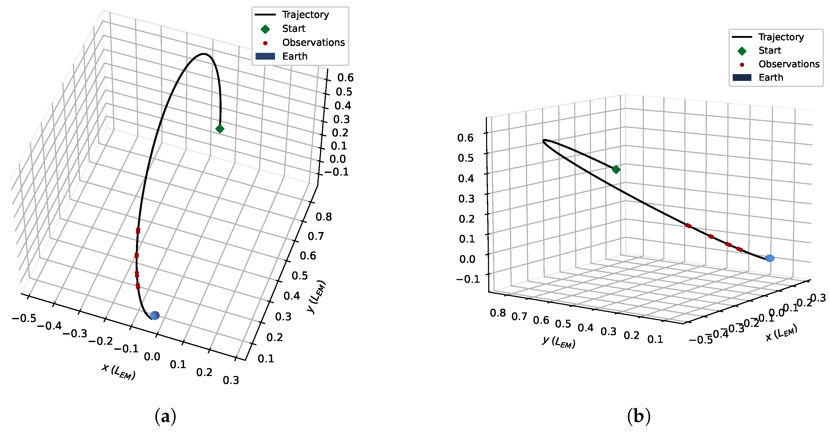
The performance of the proposed TRACER framework is evaluated on a set of real astrometric observations collected from ground-based optical sensors. The selected datasets span a range of orbital regimes and observational conditions, including geosynchronous Earth orbit (GEO), cislunar space, and heliocentric trajectories. This diversity enables a meaningful evaluation of the proposed framework across a broad range of operational scenarios, including both well-conditioned and particularly challenging cases. While the present study is not intended as a large-scale statistical benchmark against all existing orbit determination methodologies, the selected datasets were chosen to stress distinct aspects of the autonomous pipeline and to assess its robustness under realistic observational conditions.

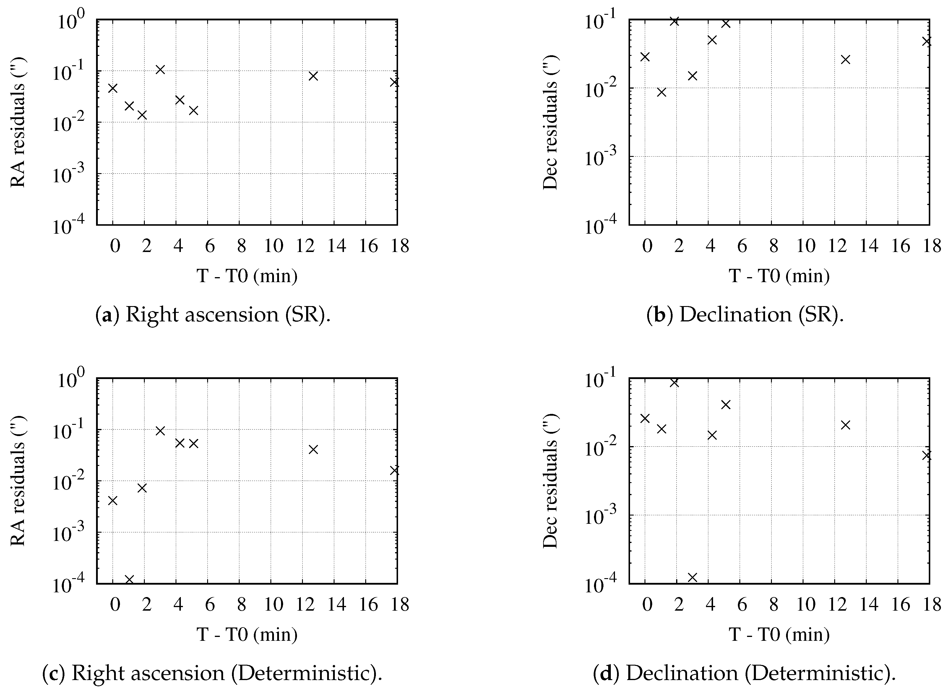
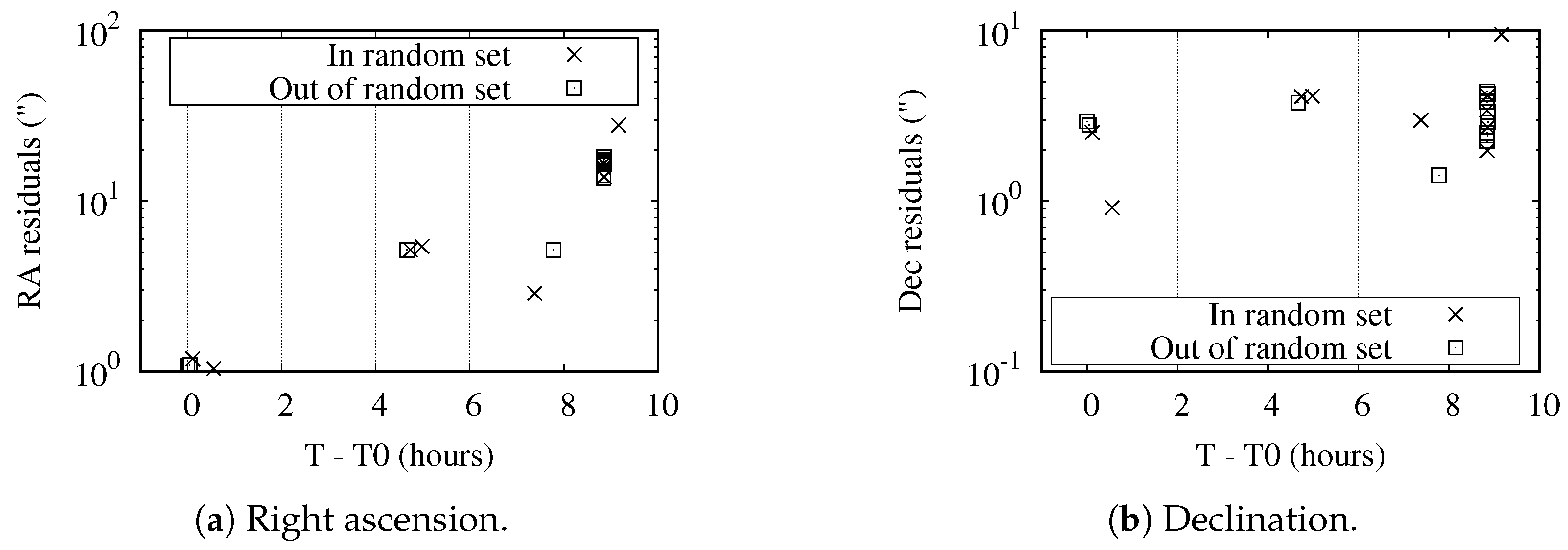
Five representative cases are considered, each characterized by different arc lengths, observation densities, and temporal distributions. In particular, the dataset includes both short-arc and long-arc regimes, as well as cases with clustered observations, which are known to be particularly challenging for angles-only orbit determination. A summary of the datasets is provided in

Table 1. Summary of observational datasets used for performance evaluation.

Case	Regime	Number of Observations	Arc Length	Notes
JUICE	Heliocentric	6	2 days	2 observation clusters
Galaxy 30	Geostationary	80	64 min	Continuous arc
Queqiao-2	Cislunar	714	23 days	4 observation clusters
Queqiao-2 (VSA)	Cislunar	8	18 min	Very short arc
Peregrine	Cislunar	23	9 h	Challenging dynamics

.

All observations consist of angular measurements in right ascension and declination, with associated timestamps. No range information is available, making the estimation problem inherently underdetermined, particularly in short-arc scenarios.

The observational datasets used in this work are not publicly available, due to institutional and third-party restrictions associated with operational telescope activities and external collaborations. Nevertheless, descriptions of the datasets and processing procedures are provided to facilitate future comparative studies using independent observations. The proposed framework is not tied to a specific sensor or proprietary data format and can be applied to generic angles-only astrometric observations.

5.1.1. Evaluation Metrics

The performance of the orbit determination process is assessed using both quantitative and qualitative criteria. The primary metric is the score S of the best candidate solution, as defined in Section 3.1. A second key metric is the unweighted root-mean-square (${\mathrm{RMS}}_{\mathrm{unw}}$) of the angular residuals, expressed in arcseconds, as defined in Equation (2). These metrics provide a direct measure of the consistency between the estimated orbit and the observed data.

In addition, other indicators are considered. First, convergence success is assessed by determining whether the algorithm identifies a physically consistent orbit that satisfies a predefined acceptance threshold on the residual score. Also, a qualitative evaluation of the algorithmic behavior is performed, analyzing the sequence of estimation steps, including the selection of IOD methods, activation of recovery strategies, and use of the randomized subset-selection mechanism.

5.1.2. Remarks on the Experimental Setup

The present experimental campaign is not intended to constitute a statistically exhaustive benchmark across the full spectrum of orbit determination methodologies. Instead, the selected case studies were designed to evaluate the behavior of the proposed framework across qualitatively distinct and operationally challenging observational regimes. Each case is analyzed in detail to illustrate the role of different components of the algorithm, including statistical ranging, deterministic IOD, recovery strategies, data filtering mechanisms, and the randomized subset-selection strategy.

Accordingly, the results should be interpreted as a representative operational validation of the proposed autonomous framework rather than as a comprehensive comparison against all existing orbit determination approaches, such as Bayesian filters, admissible-region methods, systematic ranging, or other modern estimators. Direct benchmarking against these methods would require a dedicated large-scale experimental campaign with common datasets, consistent assumptions, and comparable implementation details, which is beyond the scope of the present work.

Nevertheless, the selected datasets provide meaningful stress cases for assessing the proposed framework, since they include sparse short arcs, clustered observations, heterogeneous temporal distributions, and challenging cislunar trajectories. A broader statistical evaluation on large-scale observational datasets, including direct comparisons against alternative probabilistic and admissible-region-based frameworks, constitutes an important direction for future work.

In the following sections, the results are presented progressively, starting from well-conditioned scenarios and moving toward increasingly challenging cases, in order to elucidate the contribution of each component of the TRACER framework.

5.2. Overall Performance Summary

The performance of the proposed TRACER framework across the selected datasets is summarized in

Table 2. Summary of orbit determination performance across all test cases.

Case	Score S	${\mathbf{RMS}}_{\mathbf{unw}}$ (Arcsec)	Notes
JUICE	3.25 × 10−1	3.16 × 10−1	Deterministic IOD + Refinement is sufficient
Galaxy 30	2.86 × 10−1	6.62 × 10−1	Deterministic IOD + Refinement is sufficient
Queqiao-2	9.90 × 10−2	9.33 × 10−1	Recovery + extension required
Queqiao-2 (VSA)	6.30 × 10−2	4.15 × 10−2	Statistical ranging is successful
Peregrine	1.76 × 10−1	9.14	Randomized subset selection required

. The results highlight the ability of the algorithm to reliably converge to accurate orbit solutions under a wide range of observational conditions, including both well-conditioned and highly challenging scenarios.

As shown in Table 2, TRACER successfully converges to acceptable orbit solutions in all considered cases, including scenarios characterized by short arcs, clustered observations, and unfavorable geometric configurations. In well-conditioned cases, such as the JUICE heliocentric dataset and the Galaxy 30 geostationary arc, classical deterministic IOD methods combined with differential correction are sufficient to achieve low residual errors. In contrast, more challenging scenarios require the activation of additional components of the framework, and higher residuals are observed, particularly in the Peregrine case, which is characterized by complex dynamics and limited observation coverage.

In particular, the Queqiao-2 dataset with clustered observations necessitates the use of the recovery strategy and progressive arc extension to obtain a consistent solution across the full observation set. For very short arcs, as in the Queqiao-2 (VSA) case, the statistical ranging approach provides superior initial estimates compared to deterministic methods. Finally, in the Peregrine case, the baseline Find_Orb pipeline fails to converge to a satisfactory solution, but the randomized subset-selection strategy enables TRACER to identify a physically consistent orbit.

These results demonstrate the complementary role of the different estimation strategies within the TRACER architecture and highlight the importance of adaptive decision-making in achieving robust orbit determination across diverse observational regimes.

5.3. JUICE: Heliocentric Short-Arc Case

The JUICE (JUpiter ICy moons Explorer) spacecraft is currently on an eight-year transfer trajectory to Jupiter, exploiting multiple planetary gravity assists to achieve the required energy. Launched by the European Space Agency (ESA) on 14 April 2023, the mission performed a successful Earth–Moon double flyby between 19 and 20 August 2024.

The observations considered in this case were acquired prior to the flyby, on 7 and 9 August 2024, from the Riverland Dingo Observatory, located approximately 300 km east of Adelaide, South Australia. The dataset consists of six angular measurements (right ascension and declination), organized into two short observation arcs (one per night), each spanning less than one hour and containing three observations. This configuration results in a sparse and only moderately constrained estimation problem, which remains inherently underdetermined due to the absence of range information.

Table 3. Initial and final score and RMS for the JUICE dataset.

Method	Score S	${\mathbf{RMS}}_{\mathbf{unw}}$ (Arcsec)
SR	6.24	8.94
Gauss	1.08 × 101	3.96
Väisälä	2.53 × 101	7.97
Refinement	3.93 × 10−1	2.54 × 10−1
Outlier rejection	3.25 × 10−1	3.16 × 10−1
Final	3.25 × 10−1	3.16 × 10−1

reports the score and RMS associated with the intermediate and final solutions obtained for this dataset. In this case, the statistical ranging branch does not produce a sufficient number of candidate solutions satisfying the acceptance threshold (set to $S<0.7$), with the best candidate achieving a score of approximately $6.2$. As a result, the algorithm proceeds directly with the deterministic orbit determination pipeline.

An initial orbit is successfully obtained using Gauss’ method, yielding residuals on the order of a few arcseconds. A comparable solution is also obtained using the modified Väisälä method, albeit with higher initial residuals and score. Subsequent refinement through linear and nonlinear differential correction significantly improves the solution quality, reducing both the RMS and the score.

The recovery strategy is not activated, as the refined solution satisfies the acceptance criteria, and all observations are retained throughout the estimation process. A single observation is identified as a potential outlier during the data consistency stage; its removal results in a slight increase in the unweighted RMS residual, but a reduction in the score, which remains the primary metric for solution selection.

The post-fit residuals are shown in Figure 4 and confirm sub-arcsecond consistency across both observation arcs. For clarity, the residual magnitudes are displayed on a logarithmic scale in order to visualize residuals spanning multiple orders of magnitude within the same plot. The reconstructed trajectory, projected onto the Earth–Moon plane in the Earth–Moon synodic frame, is reported in Figure 5. For visualization purposes, the time window of the trajectory plot is shifted to 19–22 August 2024, rather than centered on the observation epochs, in order to highlight the geometry of the Earth–Moon double flyby that occurred on 19–20 August 2024.

Overall, this case illustrates that, in well-conditioned heliocentric scenarios with sufficient temporal separation between observations, classical deterministic IOD methods combined with differential correction are sufficient to achieve accurate orbit estimates. In such conditions, the additional mechanisms introduced in TRACER are not required, highlighting the adaptive nature of the framework.

5.4. Galaxy 30: Geostationary Case

Galaxy 30 is a geostationary communication satellite located at 125° West longitude. The observations considered in this case were acquired on 26 October 2023, from the Biosphere 2 Observatory near Tucson, Arizona. The dataset consists of 80 angular measurements spanning a continuous arc of approximately 64 min, corresponding to an average sampling interval of about 48 s. This configuration provides a dense set of observations over a short fraction of the orbital period, resulting in a well-constrained but geometrically limited estimation problem typical of GEO regimes.

Table 4. Initial and final score and RMS for the Galaxy 30 dataset.

Method	Score S	${\mathbf{RMS}}_{\mathbf{unw}}$ (Arcsec)
SR	3.45 × 101	3.50 × 103
Gauss	–	–
Väisälä	3.70 × 101	4.13 × 101
Refinement	2.86 × 10−1	6.62 × 10−1
Final	2.86 × 10−1	6.62 × 10−1

reports the score and RMS associated with the intermediate and final solutions. The statistical ranging branch does not produce any candidate solutions satisfying the acceptance threshold, and the algorithm proceeds with the deterministic orbit determination pipeline.

In this scenario, Gauss’ method fails to produce a valid solution, as no admissible root of the governing polynomial satisfies the required geometric constraints. This behavior is consistent with the limited angular variation over the short observation arc, which leads to poor conditioning of the Gauss formulation. In contrast, the modified Väisälä method successfully identifies an initial orbit, albeit with relatively large residuals and score.

The subsequent refinement stage, based on linear and nonlinear differential correction, significantly improves the solution quality, reducing both the RMS and the score by more than two orders of magnitude.

No recovery actions are required, as the initial solution meets the acceptance criteria, and all observations are retained throughout the estimation process. Additionally, no measurements are flagged as outliers during the data consistency stage, indicating a high level of internal consistency within the dataset. The final solution achieves sub-arcsecond accuracy for the majority of the observations, as shown in Figure 6.

Overall, this case highlights the importance of method complementarity within the TRACER framework. While Gauss’ method may fail under limited angular diversity, the Väisälä approach provides a viable alternative, enabling successful initialization. The refinement stage then plays a critical role in recovering an accurate orbit solution from a relatively poor initial estimate.

5.5. Queqiao-2 Rocket Body: Cislunar Case with Clustered Observations

The Queqiao-2 mission is a communication relay system operated by the China National Space Administration (CNSA), supporting lunar far-side and south pole operations. The spacecraft was launched on 20 March 2024, aboard a Long March 8 vehicle, which injected it into a translunar trajectory.

The observations considered in this case correspond not to the spacecraft itself, which performed lunar orbit insertion maneuvers shortly after launch, but to the associated rocket body. This object remained on a highly elliptical cislunar trajectory for several weeks before re-entering the Earth’s atmosphere on 24 April 2024.

The dataset consists of 714 angular measurements acquired from the Biosphere 2 Observatory over four distinct observation clusters (22 March, 28 March, 4 April, and 14 April 2024). The non-uniform temporal distribution of the data, combined with the long time span and the presence of significant dynamical evolution between clusters, makes this a particularly challenging orbit determination problem, requiring consistency across multiple disjoint arcs.

Table 5. Initial and final score and RMS for the Queqiao-2 rocket body dataset.

Method	Score S	${\mathbf{RMS}}_{\mathbf{unw}}$ (Arcsec)
SR	–	–
Gauss 1	1.70 × 10−1	7.08 × 103
Väisälä 1	9.28 × 10−1	7.08 × 103
Refinement	5.43 × 10−2	7.08 × 103
Extension	8.86 × 10−1	8.93 × 10−1
Outlier rejection	9.90 × 10−2	9.33 × 10−1
Final	9.90 × 10−2	9.33 × 10−1

¹ Using observations from the last cluster only.

summarizes the score and RMS at the different stages of the estimation process. Due to the long arc length (∼23 days), statistical ranging is not invoked, and the algorithm proceeds directly with deterministic IOD.

When all observations are considered simultaneously, both Gauss and Väisälä methods fail to produce a satisfactory initial orbit. Gauss yields no admissible solution, while Väisälä produces an orbit that is inconsistent with the full dataset, resulting in a very large score. This behavior reflects the difficulty of fitting a single orbit across widely separated observation clusters in the presence of significant dynamical evolution.

To address this issue, the recovery strategy is activated, progressively reducing the maximum subarc length. After three reductions, a valid initial solution is obtained using only the last observation cluster (14 April 2024), which spans approximately one hour and contains 115 observations. In this configuration, the Gauss-based solution achieves a lower score than the Väisälä solution and is therefore selected for refinement.

The refinement stage significantly improves the score, while the RMS residual remains large. This apparent discrepancy arises because the RMS is still evaluated over the full dataset, including observations that are not considered in the current subarc.

The extension strategy is subsequently activated, allowing additional clusters to be incorporated into the estimation. As more observations are included, the RMS residual drops dramatically to the sub-arcsecond level, indicating improved consistency across the dataset, while the score temporarily increases due to the inclusion of more challenging measurements.

Finally, the outlier rejection stage identifies all observations from the third cluster (4 April 2024) as inconsistent with the estimated orbit. Removing these measurements leads to a substantial improvement in the score, while the RMS remains essentially unchanged.

The post-fit residuals are shown in Figure 7, demonstrating sub-arcsecond consistency across the retained observation clusters, while the rejected cluster exhibits systematically larger residuals.

The reconstructed trajectory corresponding to the final solution is shown in Figure 8. The solution captures the highly elliptical cislunar trajectory of the rocket body, including a lunar flyby occurring between the first and second observation clusters, which induces a significant change in the orbital plane. Propagation beyond the observation window indicates atmospheric re-entry approximately one month after the first observation, consistent with the known behavior of the object.

Overall, this case highlights the importance of adaptive strategies for orbit determination in the presence of clustered observations and long dynamical evolution. The combination of subarc selection, progressive extension, and data filtering enables TRACER to recover a consistent solution in a scenario where standard approaches fail to converge.

5.6. Queqiao-2 Rocket Body: Very Short-Arc Case

To evaluate the performance of the proposed framework in the very short-arc regime, a subset of observations from the Queqiao-2 rocket body dataset is considered. Specifically, 8 observations are randomly selected from the second observation cluster (28 March 2024), corresponding to a time span of approximately 18 min.

In this configuration, the orbit determination problem is strongly underconstrained, and the statistical ranging (SR) branch is activated. A sufficient number of candidate solutions satisfying the acceptance criteria is generated, and the final solution is obtained by selecting a median orbit from the set of best candidates, as explained in Section 3.2. The resulting score and RMS are reported in

Table 6. Initial and final score and RMS for the Queqiao-2 rocket body very short arc (VSA) dataset.

Method	Score S	${\mathbf{RMS}}_{\mathbf{unw}}$ (Arcsec)
SR	5.06 × 10−2	6.06 × 10−2
Gauss 1	4.58 × 10−2	4.62 × 10−2
Väisälä 1	4.63 × 10−2	4.69 × 10−2
Refinement 1	6.30 × 10−2	4.15 × 10−2
Final (SR)	5.06 × 10−2	6.06 × 10−2

¹ Results obtained from a separate run in which the SR branch was disabled to evaluate the deterministic pipeline independently.

.

For comparison purposes, the deterministic pipeline is also evaluated by disabling the SR branch in a separate run. In this case, both Gauss’ and Väisälä methods are able to produce initial orbit estimates with similar scores and RMS values. Notably, these initial metrics are slightly better than those obtained via SR. However, this does not imply superior performance.

Indeed, the deterministic initial solutions are constructed using only a small subset of observations (typically two or three), and their associated metrics reflect consistency with this limited subset. In contrast, all SR candidate solutions are evaluated and refined using the full set of 8 observations. As a result, the SR solution directly reflects global consistency across the entire dataset.

When the deterministic solutions are subsequently refined through differential correction using all observations, their score increases, indicating a degradation in global consistency. In particular, the refined deterministic solutions exhibit worse scores than the SR-based solution, demonstrating that the latter provides a more balanced fit across the full observation arc.

The post-fit residuals for both approaches are shown in Figure 9. The SR solution achieves a more uniform distribution of residuals across all observations, whereas the deterministic solutions exhibit lower residuals at the endpoints of the arc, which are used for initialization, but larger discrepancies at intermediate epochs. This behavior highlights the tendency of deterministic IOD methods to overfit the observations used for initialization, particularly in short-arc regimes.

Overall, this case illustrates the advantage of statistical ranging in very short-arc regimes, where deterministic methods may yield solutions that are locally accurate but not globally consistent. By explicitly accounting for all observations during candidate evaluation, SR provides more robust initializations for subsequent orbit refinement.

5.7. Peregrine: Cislunar Case with Noisy Observations

The Peregrine lunar lander, developed by Astrobotic Technology, was launched on 8 January 2024, aboard a Vulcan Centaur rocket. Following separation from the launch vehicle, the spacecraft experienced a propellant leak that prevented the execution of the nominal lunar orbit insertion maneuvers. The mission was subsequently aborted, and the lander was redirected toward Earth, re-entering the atmosphere on 18 January 2024.

The observations considered in this case correspond to the Peregrine lander itself. The dataset consists of 23 angular measurements acquired from multiple ground-based observatories during the final 9 h prior to re-entry. This scenario presents several challenges: the limited number of observations, their heterogeneous origin, and the presence of non-ideal dynamical behavior due to the propellant leak and possible corrective actions. Although the short time span still permits meaningful orbit determination, the trajectory is not expected to be strictly ballistic, introducing modeling errors that impact the achievable residual accuracy.

In this case, the baseline Find_Orb pipeline does not converge to a satisfactory solution. Statistical ranging fails to generate acceptable candidate orbits, and the deterministic IOD methods are unable to identify a valid solution when applied to the full dataset. The recovery strategy, based on progressive reduction of the subarc length, is also ineffective in this context, highlighting the difficulty of the estimation problem.

In contrast, the randomized subset-selection strategy in TRACER enables recovery from this failure mode. By sampling multiple subsets of observations, the algorithm eventually identifies a subset for which the Väisälä method yields a valid initial orbit. In particular, a subset of 10 non-consecutive observations is selected, providing sufficient geometric diversity while avoiding inconsistent measurements.

Table 7. Initial and final score and RMS for the Peregrine dataset on the randomly selected subset of observations.

Method	Score S	${\mathbf{RMS}}_{\mathbf{unw}}$ (Arcsec)
SR	3.02 × 103	1.54 × 104
Gauss	–	–
Väisälä	1.56 × 10	7.08 × 103
Refinement	1.57	4.71 × 103
Extension	1.57	4.71 × 103
Outlier Rejection	1.74 × 10−1	3.04 × 103
Global Refinement	1.76 × 10−1	9.14
Final	1.76 × 10−1	9.14

summarizes the evolution of the score and RMS over the randomly selected subset that leads to a valid solution. While statistical ranging and Gauss’ method remain unsuccessful, the Väisälä method produces a valid initial orbit after the recovery strategy further reduces the subset size. Ultimately, a minimal subset of 5 observations is identified, from which a geometrically consistent solution can be obtained.

This solution is then refined through differential correction. However, direct extension to the remaining observations is initially unsuccessful, reflecting inconsistencies within the dataset. The outlier rejection stage subsequently identifies two observations as incompatible with the estimated orbit, reducing the working subset to 3 observations.

Despite the small size of this subset, the resulting solution provides a reliable initialization. A final nonlinear least-squares fit is then performed over the full dataset of 23 observations, ensuring consistency with all available measurements. This global refinement step, which is systematically applied once a valid subset-based solution is identified, enables recovery of an orbit that is compatible with the majority of the observations, despite the presence of noise and modeling errors.

The final solution achieves a low score ($S\approx 0.18$), indicating overall consistency with the retained observations, while the unweighted RMS remains on the order of ∼9 arcseconds. This relatively high residual level is attributed to a combination of measurement noise, inter-observatory biases, and model mismatch arising from unmodeled non-gravitational effects associated with the propellant leak. Importantly, the short time span of the observations limits the impact of these perturbations, allowing a meaningful orbit solution to be obtained despite these challenges.

The post-fit residuals are shown in Figure 10, where several observations exhibit errors of several arcseconds or more, consistent with the expected data quality and modeling limitations.

Forward propagation of the final solution indicates atmospheric re-entry approximately 2.5 h after the last observation (approximately 21:03 UTC on 18 January 2024), consistent with independent reports of the event. This agreement supports the physical validity of the estimated orbit despite the elevated residuals.

The reconstructed trajectory is shown in Figure 11. The integration is initialized several days prior to the observation window for visualization purposes only. Due to the presence of non-gravitational perturbations, the trajectory outside the observation interval should be interpreted qualitatively.

Overall, this case demonstrates the robustness of the TRACER framework in the presence of noisy, heterogeneous, and dynamically inconsistent observations. In particular, the randomized subset-selection strategy is essential for identifying a viable initialization in scenarios where standard orbit determination pipelines fail.

5.8. Computational Performance

In addition to solution accuracy and robustness, the computational cost of the proposed framework is an important consideration for autonomous orbit determination. This is particularly relevant for the randomized subset-selection strategy introduced in TRACER, as this procedure may repeatedly invoke the inner orbit-determination pipeline until a subset leading to an acceptable full-dataset solution is identified.

All runtime measurements reported in this section were obtained on an Intel(R) Core(TM) i9-14900K processor, running at a base frequency of 3.20 GHz, with 64 GB of RAM. The C++ implementation of the TRACER framework was compiled using g++ version 13.3.0 with the optimization flag -O3.

The timings in

Table 8. Computational performance of TRACER on the five observational datasets.

Case	Number of Observations	Active Strategy	Runtime (s)
JUICE	6	IOD + Refinement	0.46 s
Galaxy 30	80	IOD + Refinement	2.61 s
Queqiao-2	714	IOD + Recovery + Extension	10.10 s
Queqiao-2 (VSA)	8	Statistical Ranging	2.8 s
Peregrine	23	Randomized subset selection	6.52 ± 7.5 s

correspond to single-threaded execution and exclude file input/output, diagnostic logging, and plotting. For deterministic cases, each dataset was processed 10 times and the average wall-clock time is reported. For the Peregrine case, where randomized subset selection is activated, the algorithm was executed over 50 independent random seeds, and summary statistics of the resulting runtime distribution are reported.

For the JUICE and Galaxy 30 datasets, the deterministic IOD and refinement pipeline is sufficient to obtain an acceptable solution. The Queqiao-2 rocket-body case requires recovery and progressive extension, increasing the runtime, but it does not require the randomized outer loop. The Queqiao-2 very-short-arc case is successfully solved using statistical ranging. In contrast, the Peregrine case requires randomized subset selection, leading to a variable runtime distribution and, in general, a higher computational cost.

Nevertheless, the additional computational cost introduced by the randomized subset-selection strategy is conditional rather than systematic. When the inner pipeline succeeds, TRACER does not need to invoke the randomized outer loop. Only when the inner pipeline fails, the randomized strategy increases the runtime. This additional cost is the price paid for improved robustness in cases where unfavorable geometry, sparse data, outliers, or model mismatch prevent direct convergence.

For the Peregrine dataset, the variability in runtime is due to the stochastic nature of the subset-selection process. Some random seeds identify a successful subset after relatively few trials, while others require additional attempts before sampling a subset that leads to an acceptable full-dataset solution. For this reason, Table 8 reports the runtime distribution in terms of the mean and standard deviation. For completeness, the median runtime was $4.03$ s, with a range of 1.31–42.43 s over 50 random seeds. Randomized subset selection required an average of $2.84\pm 2.34$ trials, with a median of 2 and a range of 1–10 trials over the same 50 random seeds.

To further assess how the computational cost scales with the number of observations, an additional empirical scaling experiment was performed using the Queqiao-2 rocket-body dataset. This dataset was selected because it contains the largest number of measurements among the test cases and spans four separated observation clusters, providing a representative case for evaluating the dependence of runtime on dataset size. Subsets of size

$$N\in \{25,50,75,100,150,200,300,400,500,600,714\}$$

(49)

were generated using stratified random sampling across the four observation clusters, so that each subset approximately preserved the temporal distribution of the full dataset. For each value of N, the experiment was repeated over 10 random seeds, and the median runtime, along with the interquartile range, was recorded.

Figure 12 shows the resulting empirical relationship between runtime and the number of observations. The observed trend reflects the increasing cost of residual evaluation, differential correction, and validation as the number of measurements grows. However, the scaling test should be interpreted as an empirical characterization of the present implementation rather than a general asymptotic complexity analysis, since the total runtime also depends on the observation geometry, the conditioning of the initial orbit determination problem, and the number of recovery or refinement steps activated by the decision logic.

These results indicate that the computational overhead of TRACER is strongly case-dependent. For well-conditioned datasets, the framework behaves similarly to the deterministic inner pipeline. For more challenging datasets, additional recovery, extension, or randomized subset-selection steps increase the computational burden, but provide robustness that is not available from a single direct application of the baseline orbit-determination pipeline.

6. Conclusions

This work presented TRACER, a robust and autonomous framework for angles-only orbit determination designed to operate across a wide range of observational conditions. The problem of orbit determination from optical measurements remains inherently challenging due to the absence of range information, the presence of noise, and the frequent occurrence of sparse and irregular observation arcs. To address these challenges, the proposed approach integrates multiple estimation strategies within a unified, decision-driven architecture, enabling reliable orbit reconstruction without manual intervention.

A key contribution of this work lies in the combination of complementary orbit determination techniques within a coherent pipeline. Statistical ranging is employed in short-arc regimes to explore the space of admissible solutions, while deterministic methods such as Gauss’ and Väisälä techniques provide efficient initial estimates when sufficient geometric information is available. These components are coupled with a unified scoring framework that balances observational consistency and physical plausibility. Most notably, the introduction of a randomized subset-selection outer loop significantly enhances robustness by enabling recovery from failure modes associated with unfavorable observation geometry or inconsistent measurements.

The results obtained on real astrometric datasets highlight several important insights. Deterministic methods are shown to be highly effective in well-conditioned scenarios, particularly for longer observation arcs or geometries with sufficient curvature. In contrast, statistical ranging proves advantageous in very short-arc regimes, where the estimation problem is inherently underconstrained. Furthermore, the randomized subset-selection strategy plays a critical role in challenging cases, allowing the algorithm to identify consistent subsets of observations and recover valid orbital solutions even when the full dataset cannot be directly fit.

Several components of the proposed framework rely on user-defined thresholds, admissibility bounds, and empirical scoring terms. These values should be interpreted primarily as operational gates and range-definition parameters, rather than as finely tuned constants with unique physical significance. Their role is to restrict candidate generation to broad but reasonable regions of the solution space, reject clearly implausible early solutions, and prevent inconsistent observations from degrading the estimation process. The robustness of the overall OD procedure is therefore not expected to depend on the precise numerical value or analytical form of any single heuristic parameter, provided that these choices remain physically reasonable and preserve their intended qualitative role. In practice, convergence to an acceptable orbit is driven by the repeated combination of physical admissibility checks, least-squares refinement, and validation against the available observations, while the heuristic parameters serve mainly to guide the search and prevent unrealistic solutions from dominating the candidate pool.

Despite its robustness, the proposed framework presents several opportunities for further improvement. The computational cost associated with repeated subset sampling and candidate evaluation may become significant for large datasets, suggesting the need for more efficient sampling or pruning strategies. Additionally, while the scoring function incorporates physically motivated penalties, it does not provide a fully probabilistic characterization of uncertainty. Future work will therefore focus on extending the framework to include uncertainty quantification, performing systematic sensitivity analyses of the heuristic thresholds and scoring terms, and further assessing robustness across different observational regimes. Future validation efforts will also investigate the use of publicly available astrometric datasets to facilitate reproducibility studies and comparative evaluations against other orbit determination frameworks. Enabling real-time deployment within large-scale space surveillance pipelines is another important direction. Finally, the integration of data-driven techniques with the proposed physics-based framework represents a promising avenue for enhancing performance in complex and evolving operational environments.

Overall, these results suggest that the future of operational orbit determination lies not in individual algorithms, but in adaptive frameworks capable of leveraging their complementary strengths.

References

1. Gooding, R.H. A New Procedure for Orbit Determination Based on Three Lines of Sight (Angles Only); Technical Report DRA-TR-93004; Defence Research Agency Farnborough: Farnborough, UK, 1993.
2. Milani, A.; Gronchi, G. Theory of Orbit Determination; Cambridge University Press: Cambridge, UK, 2009. [Google Scholar]
3. Tapley, B.D.; Schutz, B.E.; Born, G.H. Statistical Orbit Determination; Academic Press: Burlington, MA, USA, 2004. [Google Scholar] [CrossRef]
4. Vallado, D.A. Fundamentals of Astrodynamics and Applications; Microcosm Press: Hawthorne, CA, USA, 2013. [Google Scholar]
5. Zhang, Z.; Sang, J.; Li, Z. Addressing the ill-conditioned problem in initial orbit determination via the Gooding algorithm. Astrodynamics 2025, 9, 303–320. [Google Scholar] [CrossRef]
6. Mancini, M.; Duff, T.; Leykin, A.; Christian, J.A. Geometric Solution to the Angles-Only Initial Orbit Determination Problem. J. Astronaut. Sci. 2025, 72, 49. [Google Scholar] [CrossRef]
7. Heidrich, C.; Holzinger, M. Universal Angles-Only Cislunar Initial Orbit Determination Using Sparse Grid Collocation. J. Astronaut. Sci. 2025, 72, 16. [Google Scholar] [CrossRef]
8. Feng, Z.; Yan, C.; Wu, C.; Qiao, Y. Positioning Error Estimation Method for Short-Arc Angles-Only Initial Orbit Determination. J. Guid. Control. Dyn. 2024, 47, 1072–1079. [Google Scholar] [CrossRef]
9. Virtanen, J.; Muinonen, K.; Bowell, E. Statistical Ranging of Asteroid Orbits. Icarus 2001, 154, 412–431. [Google Scholar] [CrossRef]
10. Oszkiewicz, D.; Muinonen, K.; Virtanen, J.; Granvik, M. Asteroid orbital ranging using Markov-Chain Monte Carlo. Meteorit. Planet. Sci. 2009, 44, 1897–1904. [Google Scholar] [CrossRef]
11. Muinonen, K.; Fedorets, G.; Pentikäinen, H.; Pieniluoma, T.; Oszkiewicz, D.; Granvik, M.; Virtanen, J.; Tanga, P.; Mignard, F.; Berthier, J.; et al. Asteroid orbits with Gaia using random-walk statistical ranging. Planet. Space Sci. 2016, 123, 95–100. [Google Scholar] [CrossRef]
12. Chesley, S.R. Very short arc orbit determination: The case of asteroid 2004 FU162. Proc. Int. Astron. Union 2004, 2004, 255–258. [Google Scholar] [CrossRef]
13. Farnocchia, D.; Chesley, S.; Micheli, M. Systematic ranging and late warning asteroid impacts. Icarus 2015, 258, 18–27. [Google Scholar] [CrossRef]
14. Milani, A.; Gronchi, G.F.; Vitturi, M.D.M.; Knežević, Z. Orbit determination with very short arcs. I admissible regions. Celest. Mech. Dyn. Astron. 2004, 90, 57–85. [Google Scholar] [CrossRef]
15. DeMars, K.J.; Jah, M.K. Probabilistic Initial Orbit Determination Using Gaussian Mixture Models. J. Guid. Control. Dyn. 2013, 36, 1324–1335. [Google Scholar] [CrossRef]
16. Furfaro, R.; Linares, R.; Jah, M.K.; Gaylor, D. Mapping sensors measurements to the resident space objects behavior energy and state parameters space via extreme learning machines. In Proceedings of the International Astronautical Congress, Guadalajara, Mexico, 26–30 September 2016. [Google Scholar]
17. Peng, H.; Bai, X. Improving orbit prediction accuracy through supervised machine learning. Adv. Space Res. 2018, 61, 2628–2646. [Google Scholar] [CrossRef]
18. Peng, H.; Bai, X. Artificial Neural Network-Based Machine Learning Approach to Improve Orbit Prediction Accuracy. J. Spacecr. Rocket. 2018, 55, 1248–1260. [Google Scholar] [CrossRef]
19. Zhang, Z.; Shi, Y.; Zheng, Z. Improving Angle-Only Orbit Determination Accuracy for Earth–Moon Libration Orbits Using a Neural-Network-Based Approach. Remote Sens. 2024, 16, 3287. [Google Scholar] [CrossRef]
20. Gong, B.; Ma, Y.; Zhang, W.; Li, S.; Li, X. Deep-neural-network-based angles-only relative orbit determination for space non-cooperative target. Acta Astronaut. 2023, 204, 552–567. [Google Scholar] [CrossRef]
21. Raissi, M.; Perdikaris, P.; Karniadakis, G. Physics-informed neural networks: A deep learning framework for solving forward and inverse problems involving nonlinear partial differential equations. J. Comput. Phys. 2019, 378, 686–707. [Google Scholar] [CrossRef]
22. Scorsoglio, A.; Ghilardi, L.; Furfaro, R. A physic-informed neural network approach to orbit determination. J. Astronaut. Sci. 2023, 70, 25. [Google Scholar] [CrossRef]
23. Scorsoglio, A.; D’Ambrosio, A.; Ghilardi, L.; Furfaro, R.; Reddy, V. Physics-informed orbit determination for cislunar space applications. In Proceedings of the Advanced Maui Optical and Space Surveillance (AMOS) Technologies Conference, Maui, HI, USA, 19–22 September 2023. [Google Scholar]
24. Scorsoglio, A.; D’Ambrosio, A.; Le Corre, L.; Gray, B.; Reddy, V.; Furfaro, R. Physics-informed orbit determination for X-GEO space situational awareness. Acta Astronaut. 2026, 238, 271–285. [Google Scholar] [CrossRef]
25. Agostinelli, I.; Goracci, G.; Curti, F. Initial orbit determination via artificial intelligence for too-short arcs. Acta Astronaut. 2024, 222, 609–624. [Google Scholar] [CrossRef]
26. Goracci, G.; Agostinelli, I.; Curti, F. Adaptive Physics-Informed Initial Orbit Determination for Too-Short Arcs From Space Optical Observations. IEEE Trans. Aerosp. Electron. Syst. 2025, 61, 10758–10767. [Google Scholar] [CrossRef]
27. Schildknecht, T. Optical surveys for space debris. Astron. Astrophys. Rev. 2007, 14, 41–111. [Google Scholar] [CrossRef]
28. Denneau, L.; Jedicke, R.; Grav, T.; Granvik, M.; Kubica, J.; Milani, A.; Vereš, P.; Wainscoat, R.; Chang, D.; Pierfederici, F.; et al. The Pan-STARRS Moving Object Processing System. Publ. Astron. Soc. Pac. 2013, 125, 357. [Google Scholar] [CrossRef]
29. Zhao, G.; Liu, L.; Li, B.; Li, Z.; Sang, J. An orbit determination approach to associating optical tracklets of space objects. Acta Astronaut. 2022, 200, 506–523. [Google Scholar] [CrossRef]
30. Gong, B.; Wang, S.; Li, S.; Li, X. Review of space relative navigation based on angles-only measurements. Astrodynamics 2023, 7, 131–152. [Google Scholar] [CrossRef]
31. Willis, M.; D’Amico, S. Fast angles-only relative navigation using polynomial dynamics. Adv. Space Res. 2024, 73, 5484–5500. [Google Scholar] [CrossRef]
32. Liao, A.R.; Oguri, K. Autonomous Shape-Free Small-Body Navigation Using Relative Angles-Only Measurements. J. Spacecr. Rocket. 2026, 63, 677–685. [Google Scholar] [CrossRef]
33. Minor Planet Center. MPCORB Database. Available online: https://minorplanetcenter.net/iau/MPCORB.html (accessed on 10 April 2026).
34. Boulet, D.L. Methods of Orbit Determination for the Microcomputer; Willmann-Bell, Incorporated: Richmond, VA, USA, 1991. [Google Scholar]
35. Väisälä, Y. Eine Einfache Methode der Bahnbestimmung; Astronomical-Optical Institute of the University of Turku Informo: Turku, Finland, 1939; Volume 1. [Google Scholar]
36. Dubyago, A.D. Determination of Elliptic Orbits. In The Determination of Orbits; Burke, R.D., Gordon, G., Rowell, L.N., Smith, F.T., Trans.; Macmillan: New York, NY, USA, 1961; Chapter 7; pp. 192–195. [Google Scholar]
37. Fischler, M.A.; Bolles, R.C. Random sample consensus: A paradigm for model fitting with applications to image analysis and automated cartography. Commun. ACM 1981, 24, 381–395. [Google Scholar] [CrossRef]
38. Danby, J.M.A. Fundamentals of Celestial Mechanics, 2nd ed.; Willmann-Bell, Incorporated: Richmond, VA, USA, 1988. [Google Scholar]
Figure 1. High-level architecture of the Find_Orb-based orbit determination pipeline.
Aerospace 13 00518 g001
Figure 2. High-level architecture of the TRACER orbit determination pipeline.
Aerospace 13 00518 g002
Figure 3. Two-dimensional density of semimajor axis and inclination for objects in the Minor Planet Center (MPC) database [33].
Aerospace 13 00518 g003
Figure 4. Post-fit residuals for the JUICE dataset.
Aerospace 13 00518 g004
Figure 5. Reconstructed trajectory in the Earth–Moon synodic frame for the JUICE dataset based on the final orbit solution.
Aerospace 13 00518 g005
Figure 6. Post-fit residuals for the Galaxy 30 dataset.
Aerospace 13 00518 g006
Figure 7. Post-fit residuals for the QQ-2A case.
Aerospace 13 00518 g007
Figure 8. Reconstructed trajectory for the QQ-2A rocket body, showing close approaches (CAs) to the Earth and Moon. (a) View approximately normal to the Earth–Moon plane. (b) Inclined perspective highlighting out-of-plane motion.
Aerospace 13 00518 g008
Figure 9. Post-fit residuals for the Queqiao-2 VSA case for both the SR and deterministic methods.
Aerospace 13 00518 g009
Figure 10. Post-fit residuals for the Peregrine dataset.
Aerospace 13 00518 g010
Figure 11. Reconstructed trajectory for the Peregrine lander. (a) View approximately normal to the Earth–Moon plane. (b) Inclined perspective.
Aerospace 13 00518 g011
Figure 12. Empirical computational scaling of TRACER with respect to the number of observations using stratified random subsets of the Queqiao-2 rocket-body dataset.
Aerospace 13 00518 g012