


Abstract
The design of millimeter-scale micro-turbine blades is challenging due to conflicting requirements: achieving aerodynamic performance while remaining compatible with microfabrication, and exploring high-dimensional morphological design spaces without prohibitive computational cost. To address these challenges, this study proposes an intelligent framework for the design and optimization of the three-dimensional blade profile of a 3 mm diameter micro-turbine. The blade morphology is parameterized using 22 variables, ensuring geometric feasibility for micro-EDM (Electrical Discharge Machining) fabrication. A physics-informed neural network (PINN) surrogate model, efficiently trained through a two-stage active learning strategy combining KD-tree exploration and residual-based sampling, provides accurate predictions of flow fields. Multi-objective optimization using Non-dominated Sorting Genetic Algorithm II (NSGA-II) is then performed to maximize torque and thrust. Experimental results show that the optimized blade achieves a 38.6% increase in rotational speed while retaining 75.1% of thrust at 0.2 MPa inlet pressure, validating the framework’s effectiveness. This methodology offers a systematic solution for designing microfluidic devices characterized by high-dimensional parameters and high-fidelity simulation requirements.
1. Introduction
Over the past two decades, micro aerial vehicles (MAVs) have developed rapidly and have found wide applications in both industrial and scientific fields [1]. However, there are still many challenges to overcome in this domain, and one of the main focuses of MAVs development today is the design of compact and efficient micro-propulsion systems that can provide both thrust and power supply [2]. Millimeter-scale micro-turbines are regarded as one of the most promising solutions for compact micro-propulsion, thanks to their high energy density and simple structure [3]. Nevertheless, miniaturizing turbines to millimeter-scale diameters faces two closely related, unresolved challenges. First, the design process is tightly coupled with manufacturing constraints: increasing geometric complexity enhances aerodynamic performance but significantly raises fabrication difficulty, while employing specialized processes to reduce size often requires compromising structural or functional features. Second, there is a lack of established design guidelines for optimizing turbine morphology at this scale, and advanced intelligent design methods have yet to be applied to address the high-dimensional, micro-scale flow problems inherent in micro-turbine optimization.
Kang et al. [4] developed a micro gas turbine with a wheel diameter of 12 mm. To enable the turbine to withstand complex stresses at high temperatures without the need for auxiliary cooling, the impeller and rotor shaft were made from silicon nitride ceramic material. Their complex micro three-dimensional structure was fabricated using a combination of shape deposition and gel casting techniques [5,6]. Yoshida et al. [7] developed a micro-turbine with a diameter of 8 mm. Isomura et al. [8] designed a micro-turbine with a diameter of 10 mm, where the impeller was processed using micro-milling techniques [9], and the rotor shaft was supported by ZrO2 ceramic hydrostatic bearings [10,11]. Peirs et al. [12] developed a single-stage axial micro gas turbine with a wheel diameter of 10 mm, which was made from stainless steel and fabricated using electrical discharge machining. Keding et al. [13] developed a turbine expander with a wheel diameter of 30 mm. These studies primarily employed three-dimensional fabrication techniques. Due to challenges in material performance and processing capabilities, most turbines in these studies have diameters greater than 10 mm, making it difficult to scale down further. These studies largely relied on conventional design approaches, which allowed for high three-dimensional freedom in blade geometry but imposed significant manufacturing challenges. As a result, most of the turbines reported have diameters greater than 10 mm, and further miniaturization remains difficult.
Waitz et al. [14] used deep reactive ion etching and wafer bonding techniques to process single-crystal silicon wafers, developing a micro radial turbine with a diameter of 4 mm. The multi-layer two-dimensional parts created by photolithography were combined to form the micro turbine engine. Based on similar process methods, Shan et al. [15] designed a micro turbine driven by compressed air, consisting of three layers of silicon wafers and two layers of acrylic plates, with a turbine diameter of 8.4 mm and a thickness of 0.76 mm. The primary structure was fabricated using photolithography, and the engine was designed to be flat. Fu et al. [16] developed a micro turbine with a diameter of 10 mm, fabricated using micro-milling techniques. It was assembled into a micro gas turbine for cold model testing [17]. Subsequently, a systematic design process for radial turbines at this scale was developed [18,19], highlighting the significant influence of rotor weight, turbine type, geometric dimensions, and manufacturing processes on turbine performance [20]. Holmes et al. [21] developed a micro axial turbine with a wheel diameter of 12 mm, designed for power generation and flow sensing applications in compact power conversion devices. A common feature of these studies is that, while advanced microfabrication techniques enable the production of smaller-diameter turbines, they often require substantial compromises in design freedom. Consequently, most designs adopt quasi-two-dimensional, flat structures, which restrict the aerodynamic optimization of fine features such as blades and limit overall turbine performance.
The aforementioned studies vividly highlight a persistent challenge in micro-turbine design: the trade-off between design flexibility and manufacturing feasibility. On one hand, three-dimensional designs with high degree of freedom allow for aerodynamic optimization of components like blades, but they often lead to complex manufacturing challenges. On the other hand, simpler, quasi-two-dimensional designs are easier to fabricate but limit the aerodynamic performance of critical components, such as blades, which negatively impacts turbine efficiency. Therefore, finding the optimal balance between these two factors is crucial to overcoming the current limitations in micro-turbine development.
In addition to the mutual constraints between manufacturing and design, micro-turbine design with millimeter-scale diameters exceeds the scope of existing theories and empirical models, necessitating novel approaches to geometric design. Modern optimization techniques, coupled with high-fidelity surrogate models, offer a way to simulate and compare the performance of various turbine geometries in a cost-effective virtual environment. However, the three-dimensional complexity of micro-turbine structures and the unique characteristics of microscale fluid flows present significant challenges in developing surrogate models that balance both cost and accuracy. Physics-informed neural networks (PINN) offer an emerging solution for efficient and high-fidelity modeling and optimization of fluid machinery by embedding physical laws, such as the governing equations, into the neural network loss function [22]. Gao et al. [23] applied PINN to construct a dual-branch classification network integrating physical mechanisms, which, in combination with computational fluid dynamics (CFD)-calibrated multibody dynamics models and generative adversarial networks (GAN), can achieve high-precision diagnostics with minimal experimental data. Li et al. [24] developed the LS-PINN framework, which combines PINN with long short-term memory (LSTM) networks to efficiently solve the fluid-structure-thermal coupling problem of turbine blades. This framework also leverages transfer learning to enable rapid field predictions under data-scarce conditions. Wang et al. [25] and Tong et al. [26] explored complex flows such as 3D airfoils and propeller unsteady wakes by deeply integrating PINN with DeepONet or convolutional LSTM autoencoders, which significantly improved the accuracy and efficiency of spatiotemporal evolution predictions. Rahman et al. [27] combined high-dimensional computing with ridge regression and applied physical constraints like thin-wing theory to achieve lightweight, interpretable, and physically consistent aerodynamic coefficient predictions for airfoils. Xiao et al. [28] incorporated the RANS (Reynolds-Averaged Navier–Stokes) equations and SST (Shear Stress Transport) turbulence model into PINN, successfully simulating compressible turbulence in rocket engine nozzles, while using transfer learning strategies to significantly reduce data requirements and computational costs. These studies demonstrate that PINN possesses the capability to rapidly compute flow field characteristics and, as such, hold great promise as an ideal surrogate model for driving the intelligent design of micro-turbines.
A review of the current state of research indicates that the miniaturization of micro-turbines to millimeter-scale diameters faces two primary challenges. The first is the intrinsic trade-off between manufacturing capabilities and design flexibility, and the second is the lack of design methodologies capable of addressing scenarios beyond the coverage of traditional theories. In this study, we focus on a 3 mm-diameter micro-turbine fabricated via three-axis micro-electrical discharge milling and propose a blade morphology parameterization method constrained by manufacturing requirements, aiming to maximize three-dimensional design freedom while ensuring process feasibility. Based on the resulting high-dimensional design space, modern intelligent algorithms are employed to optimize the turbine’s performance, targeting a balanced trade-off between rotational speed and thrust. The workflow begins with fabrication and performance testing of ten initial reference turbine samples, which are used to establish a virtual mapping between design parameters and performance via CFD simulations, forming the basis for training a PINN model. To enhance the predictive accuracy of the model, an active learning strategy is adopted, incrementally enriching the training dataset to 500 high-quality CFD samples. Finally, the established PINN surrogate model is coupled with a heuristic search algorithm to achieve balanced optimization of key performance metrics, and the resulting optimized design is experimentally validated. Through this approach, we present a fully integrated, end-to-end design methodology for micro-turbines, offering a paradigm with potential for broader application in similar microfluidic and micro-propulsion systems.
2. Materials and Methods
This section first clarifies the micro-EDM (Electrical Discharge Machining) fabrication constraints to define the blade design feasible domain, then establishes the fabrication-aware parametric model of the 3 mm micro-turbine. Subsequently, the aerodynamic performance test platform and numerical simulation method are introduced, followed by the construction of the PINN surrogate model and the multi-objective optimization framework for blade profile.
2.1. Micro-Turbine Fabrication Process and Manufacturing Constraints
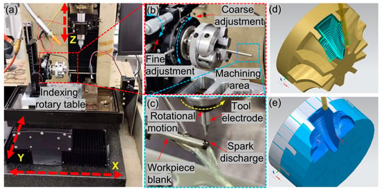
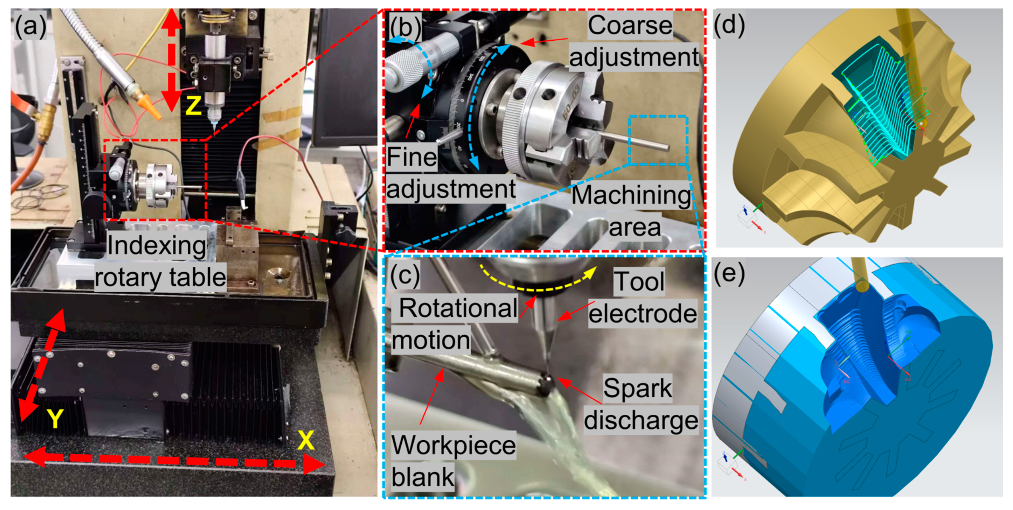
Unlike conventional-scale turbines, the geometric design of millimeter-scale micro-turbines must be strictly subject to micro-fabrication feasibility, which directly defines the feasible domain of blade profile parameters. This section first clarifies the adopted micro-EDM process and the corresponding non-negligible manufacturing constraints for subsequent design work. The network microstructure titanium matrix composites (Ti6Al4V + 5 vol.% TiBw) developed by Huang et al. [29] are used in this paper due to their light weight, high-temperature resistance, and other favorable properties, making them an ideal material for the micro-turbine. The fabrication of the turbine involves machining a complex three-dimensional surface of the heterogeneous material at a micro-scale, which presents significant challenges for traditional manufacturing methods. Therefore, a micro-EDM technique is employed to process the micro-turbine structure. The entire machining process is carried out on a three-axis micro-EDM machine developed by Harbin Institute of Technology, as shown in Figure 1a. This machine is capable of achieving a repeatability precision of 0.1 μm in the XYZ directions. Since the turbine structure has rotational symmetry, indexing milling is applied to machine different regions of the blades sequentially. The workpiece clamping system, shown in Figure 1b, connects the rotary table to the workpiece, allowing machining at different angles on the three-axis machine. The angle error is controlled within 0.05° through a coarse and fine adjustment system. The specific machining process, shown in Figure 1c, uses high-energy pulses generated by spark discharge to melt and remove metal material, without producing significant macro forces, making it ideal for fabricating small-scale, complex structures. Figure 1d shows the tool path at a single indexed position, and Figure 1e illustrates the simulated machining result (NX 12.0, Siemens Product Lifecycle Management Software Inc., Plano, TX, USA). After machining the blade area at a single position, the indexing table is rotated to the next position, and the process continues until all blade areas are machined.
Figure 1.
Indexing milling-based micro-EDM fabrication process of a micro turbine: (a) Machining equipment (b) Indexing rotary table (c) Machining area (d) Toolpath at a single indexed position (e) Simulated machining result.
Considering the practical manufacturing cost, the design problem of the turbine blades is simplified by introducing the following two basic assumptions:
1. All blades have the same structure, meaning that the impeller has rotational symmetry with respect to its axis. If the number of blades is n, the rotation angle of each blade is ;
2. There is no thickness variation between different positions on the same blade, meaning that the blade’s thickness remains constant across the three-dimensional surface.
The micro-EDM fabrication process and the associated assumptions described above define the practical manufacturing constraints for the micro-turbine. Consequently, all subsequent parametric design and optimization efforts in this work are conducted within these constraints. This approach ensures that the optimized geometries remain fully compatible with the established machining process, while providing a clear and well-defined basis for the selection of design variable bounds during the optimization stage.
2.2. Turbine Design and Blade Geometry
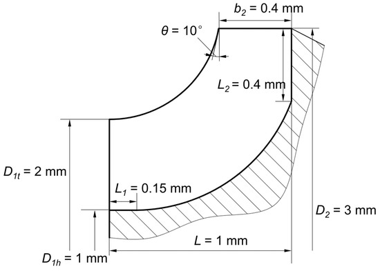
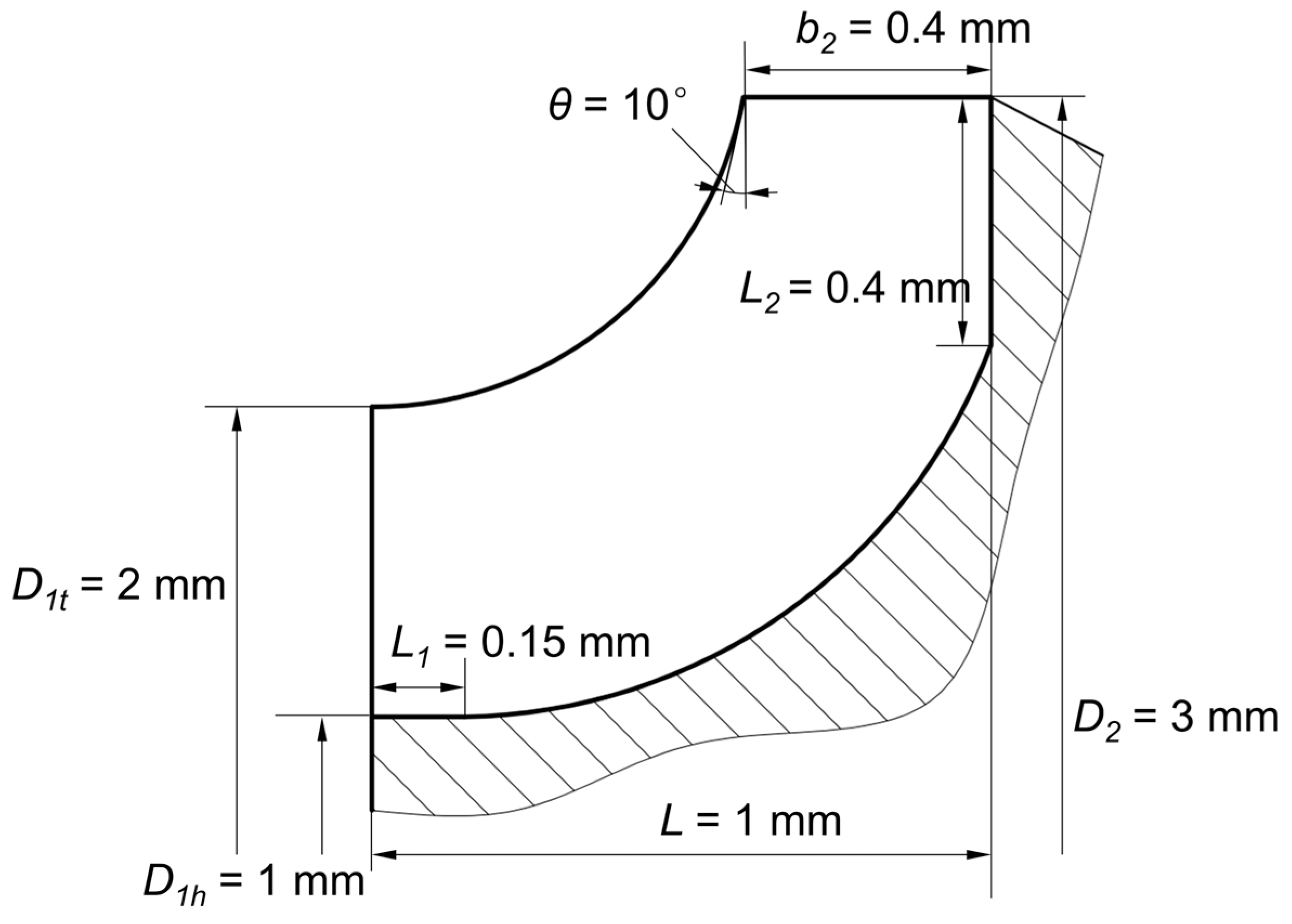
The turbine considered in this paper has a diameter of 3 mm. Due to the limited axial size of the micro-turbine rotor, a single-stage centrifugal design was adopted. The preliminary geometric parameters of the turbine’s shaft surface are initially designed, as shown in Figure 2.
Figure 2.
Geometric parameters of the turbine shaft cross-section.
Based on the determination of the outer dimensions of the impeller, it is only necessary to design the three-dimensional shape of the blade surface. By combining the number of blades n and thickness t, the structure of the impeller can be determined. Since the blade surface often has a complex spatial structure, a transformation is first applied to the space at the blade rim to extract the surface features.
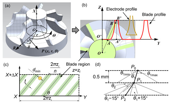
As shown in Figure 3a, the X-direction is defined along the direction from the hub axis of the impeller to the trailing edge of the blade, with the origin located on the leading-edge bottom plane. The circumferential direction is represented by polar coordinates. All length and angle coordinates are expressed in millimeters (mm) and radians (rad), respectively. At this point, any point P on the impeller can be expressed as:
Figure 3.
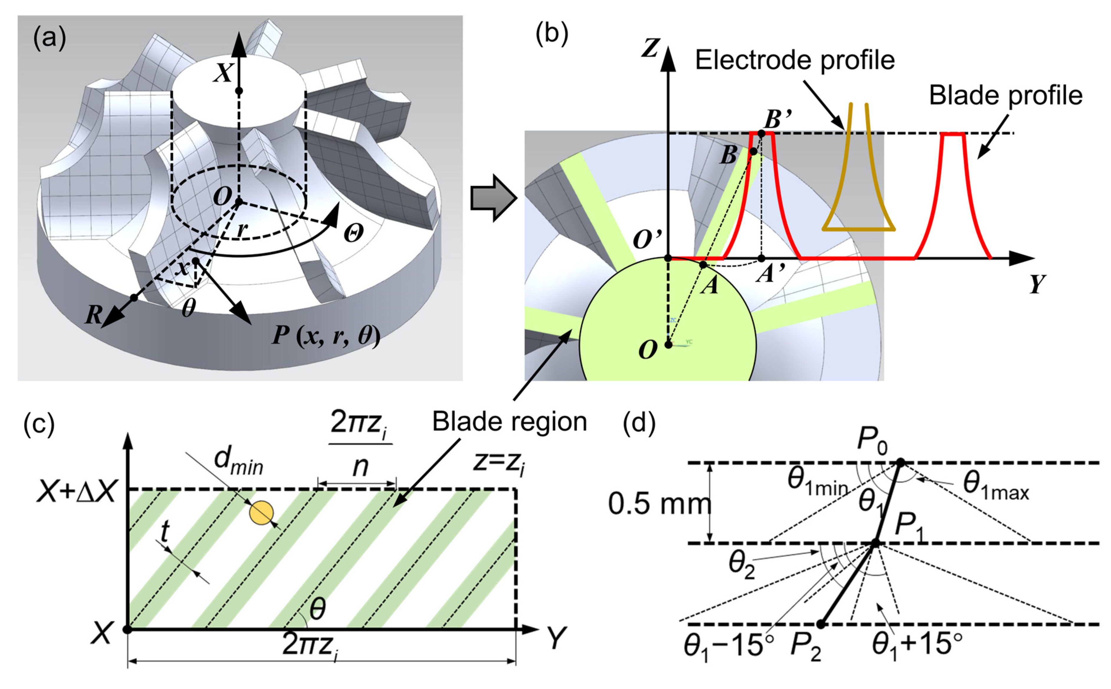
Extraction of blade profile parameters: (a) Original coordinate system (b) Transformed coordinate system (c) Geometric constraints of parameters (d) Local blade profile definition.
To facilitate subsequent calculations, the space of the impeller is mapped to a Cartesian coordinate system, with the direction of the X-axis and the position of the origin O unchanged. Figure 3b illustrates the process of transforming the bottom plane’s polar coordinate system to the yOz plane coordinate system: In the cross-sectional view of a plane along the vertical axis of the impeller, the tangent at the edge of the shaft is taken as the Y-direction, and the direction through the tangential point and along the outward diameter is taken as the Z-direction. The origin O’ is located at the tangential point, and the coordinate values are expressed in millimeters (mm). The range of Z-values is [0, 1.5], where z = 1.5 corresponds to the circumferential path of the outer diameter of the impeller. After flattening the circumference into a straight line, the position of each point along the Y-direction is obtained. Other values of z correspond to a circle with the center at the impeller’s center and a radius of z. These circles are flattened and then scaled by a certain factor to match the length of the outer diameter’s circumference. The mathematical expression for this transformation is as follows:
The key feature of the transformation is that the line passing through the diameter in the original coordinate system is transformed into a line perpendicular to the Y-direction. After the cylindrical electrode enters the impeller area, the transformed profile is shown as the brown curve in Figure 3b. Clearly, to achieve machining on a three-axis machine tool, it is necessary to ensure that the curve representing the blade profile in Figure 3b is a single-valued function with respect to y. To ensure this, the blades designed in this study have a line of intersection between the blade’s center surface and any axial cross-section that is a straight line passing through the axis.
For an impeller with n blades and thickness t, consider a differential element along the axis direction. The xOy plane view of the element at diameter zi is shown in Figure 3c. Since the scale of the element in the X-direction approaches zero, the blade profile contained within this section can be approximated as a straight line. To ensure that the blade profile can be accurately processed, it is essential that the tool electrode can pass through the gap between adjacent blades when the diameter is at its minimum. Based on the geometric relationships shown in Figure 3c, it is easy to derive that any position on the blade must satisfy the following condition:
In the equation,
θ—the tilt angle of the blade centerline;
dmin—the minimum electrode diameter, taken as 0.1 mm.
This paper limits the number of blades to be no less than 5, with the blade thickness ranging from 0.1 mm to 0.3 mm. When θ is set to 90˚, the maximum number of blades can be obtained as 15. In the design of the blade profile, since the center surface of the blade is a straight line passing through the axis in different axial sections, based on the transformation relationships shown in Figure 3a,b, it can be seen that the tilt angle of the centerline projected on the xOy plane does not depend on the position z. Therefore, the variation in the blade profile is determined solely by the centerline shape in the xOy plane.
In the specific design of the blade profile, an integer value for the number of blades is chosen within the range [5, 15]. Next, as shown in Figure 3d, the X-direction is divided into 20 equal segments, each with a length of 0.05 mm. The blade centerline is then approximated as 20 line segments with 21 nodes. Based on the axial geometric parameters shown in Figure 1, the minimum diameter corresponding to the points on the blade at different positions along the X-direction can be calculated. The tilt angle limits of the centerline at each point can be obtained by substituting into Equation (3).
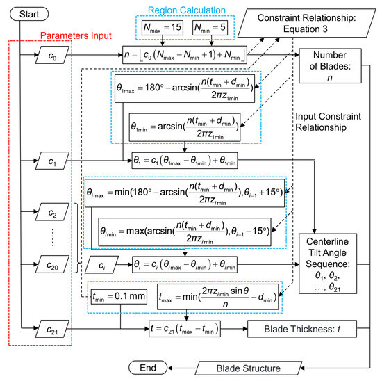
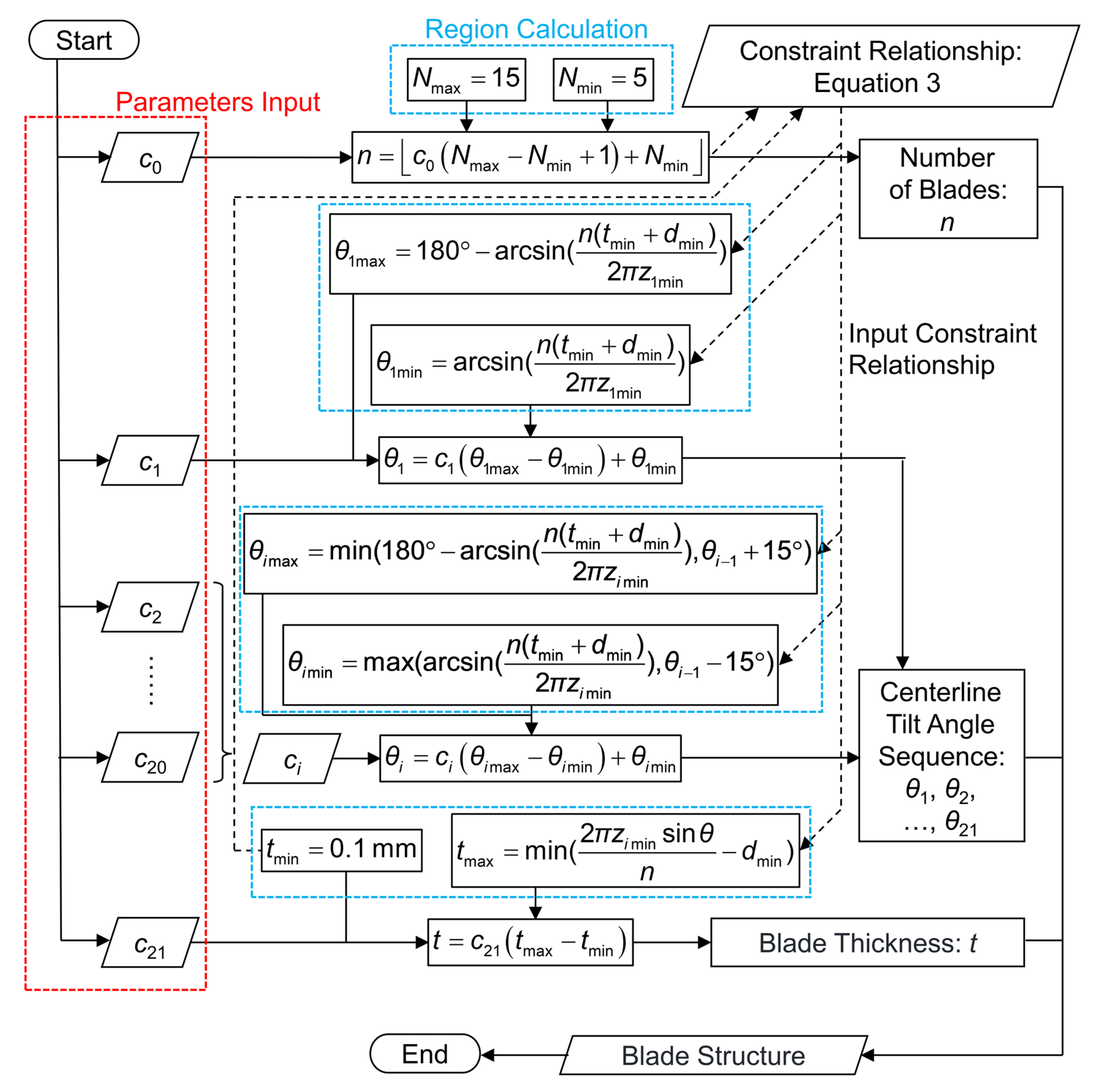
For the first node P0, with coordinates (x, y) = (0, 0), the allowable angle range between the segment P0P1 and the Y-direction is constrained within the limits obtained from Equation (3). For the other line segments PiPi+1, in addition to the restriction from Equation (3), to ensure the smoothness of the blade surface, the angle between the new segment and the previous segment should not exceed 15°. These conditions determine that the 20 line segments along the centerline can be defined by tilt angles within 20 specific ranges. Once all tilt angle values are determined, the blade thickness at each point can be derived from Equation (3). Thus, the entire blade profile can be determined by 22 coefficients [c0, c1, …, c21], each corresponding to a range [0, 1] and multiplying them by their respective value domains gives the unique impeller structure. Figure 4 illustrates the entire process of micro-turbine blade shape parameterization and structural calculation, as outlined in the preceding discussion, from input parameters to the final blade structure definition.
Figure 4.
Process flow for micro-turbine blade shape parameterization and structural calculation.
After determining the main parameters of the impeller profile, it is necessary to first select 10 initial samples in the 22-dimensional sample space for processing and actual performance testing. Since the cost of processing is high and it is not feasible to cover a large number of samples, the selected 10 samples should reflect the overall situation within the parameter space as much as possible. Therefore, a cubic hyper-Latin method is used to extract the initial samples from the parameter space. The specific process is as follows:
First, let nc represent the total number of samples (10), and mc represent the number of parameters (22). Then, the value range of each parameter is evenly divided into nc intervals. Define the following function:
where
i—the interval code, with a range of [1, nc − 1].
The lower limit of each coefficient’s partitioned interval is:
where:
L—the lower limit of each parameter’s value range, which is 0;
H—the upper limit of each parameter’s value range, which is 1;
l—the lower limit of each partitioned parameter’s value range.
Correspondingly, the upper limit of each coefficient’s partitioned interval is:
where:
h—the upper limit of each partitioned parameter’s value range.
Define η as a random number within the range [0, 1], which is used as the coefficient for determining the representative value of each interval. Thus, the random representative value for each interval is:
2.3. Experimental Setup for Performance Testing
To evaluate and optimize the aerodynamic performance of the micro-turbine, two key performance indicators—rotational speed and thrust—are selected as the primary objectives for optimization. These two indicators directly determine the power output and propulsion capability of the micro-turbine for MAV applications, which are the core performance requirements for the target scenario, and thus are selected as the primary optimization objectives. Therefore, to evaluate the performance of the initial micro samples, we first conducted physical testing focused on these two key indicators. In particular, a specially designed and fabricated micro volute was created as the functional carrier and flow path constraint component for aerodynamic testing. The structure of the micro volute is shown in Figure 5. It adopts a split design to house the micro turbine, and compressed air is introduced through the inlet to drive the turbine’s rotation. The assembly and fixation are achieved using precision small-diameter bolts and nuts, ensuring flow path sealing and structural rigidity. After assembly, the entire device’s longest dimension is approximately 12 mm. With this housing structure, compressed air can be effectively guided into the turbine area, achieving stable driving of the micro turbine and providing the necessary assembly and operating conditions for subsequent performance tests and experimental measurements.
Figure 5.
Assembly process of the micro-turbine housing: (a,b) Housing components before assembly (c,d) Housing with assembled micro-turbine.
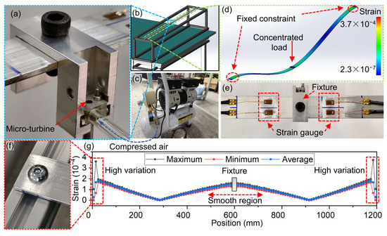
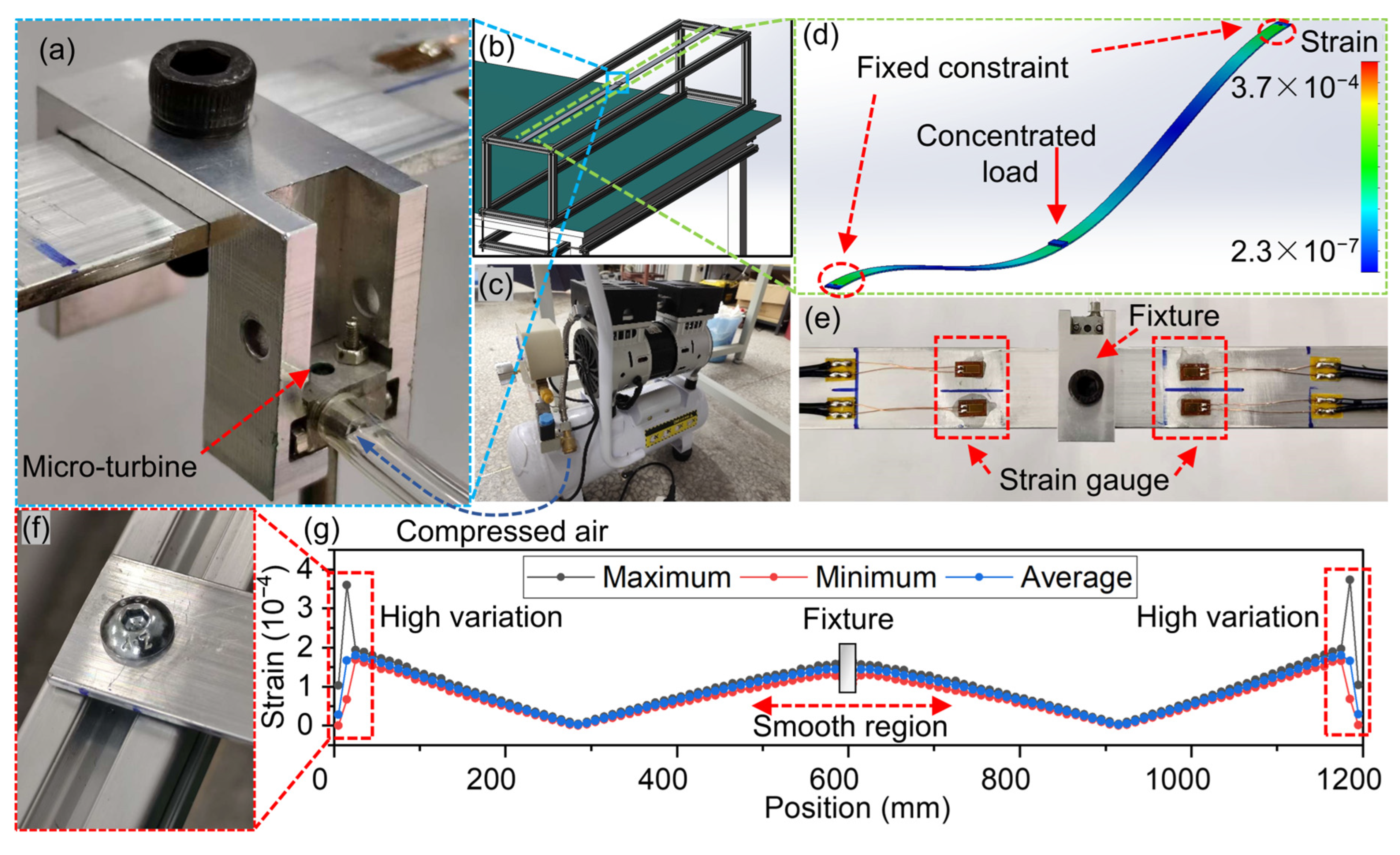
To test the aerodynamic performance of the micro impeller, an experimental platform was built, as shown in Figure 6. During testing, the micro impeller housing assembly is mounted onto the dedicated connection base in Figure 6a, and the base is connected to the central strain beam on the platform body made from the frame profile in Figure 6b. A DAERTUO 550-9L compressed air pump (Wenling Shenba Air Compressor Manufacturing Co., Ltd., Taizhou, China) is used as a stable air source, providing compressed air within the pressure range of 0~0.8 MPa. The compressed air is introduced via an external air pipe to drive the impeller, which rotates at high speeds in the air. To isolate high-frequency vibrations from the air source that could affect the test frame, a flexible PTFE (polytetrafluoroethylene) hose is used to connect the external air pipe. During this process, the impeller’s rotational speed is precisely measured non-contact using a high-speed camera model YVVSION-0SG030-790UM (with a maximum frame rate of 6600 frames per second, Shenzhen Yingshi Technology Co., Ltd., Shenzhen, China).
Figure 6.
Experimental setup for testing the micro-turbine: (a) Micro-turbine fixture (b) Testing frame (c) Compressed air system (d) Strain simulation on aluminum strips (e) Strain gauge arrangement (f) Strain beam end constraint (g) Strain data.
During the testing process, the gas is discharged from the impeller outlet, generating thrust. This thrust is transmitted through the connecting structure to an aluminum beam of 1200 mm length in the platform frame, causing micro-strain in the beam. To assess the strain response characteristics of the beam in different regions, a simulation analysis (Solidworks 2024, Dassault Systèmes SolidWorks Corporation, Waltham, MA, USA) was first performed. Figure 6d shows the strain distribution of the beam when fixed at both ends and subjected to a 1 N concentrated load at the center. The axial strain distribution analysis is shown in Figure 6g. The strain peaks are mainly located near the constrained ends. However, the strain values at these positions exhibit significant fluctuations, and the area is influenced by the assembly structure shown in Figure 6f, leading to substantial interference in the actual strain signal.
Therefore, to obtain stable and reliable strain data, strain gauges (Shanghai Chengke Electronic Technology Co., Ltd., Shanghai, China) were placed in the smoother, higher-strain middle region of the beam, as indicated in Figure 6g. The four strain gauges shown in Figure 6e were used to measure the micro-strain values. The average value of the measurements from the four strain gauges was taken as the actual strain for that position, which helps to suppress the influence of individual strain gauge data interference. During each test, once the turbine reached a stable rotational speed, strain signals were continuously recorded at a sampling frequency of 1 kHz for 30 s. The mean value of the middle 20 s of steady-state data was then taken as the final thrust measurement, reducing the impact of random fluctuations in the signal. This procedure enables accurate calculation of the thrust generated by the gas acting on the impeller.
2.4. Numerical Simulation and Performance
While high-quality experimental data on turbine performance can be obtained for various blade parameters, this process involves significant fabrication and testing costs, making it difficult to cover a larger sample space. Therefore, it is necessary to develop more efficient surrogate models that enable the mapping of blade parameters to turbine performance over a broader range with high efficiency.
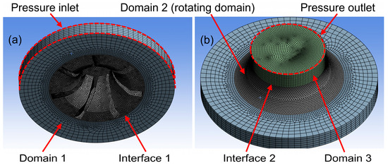
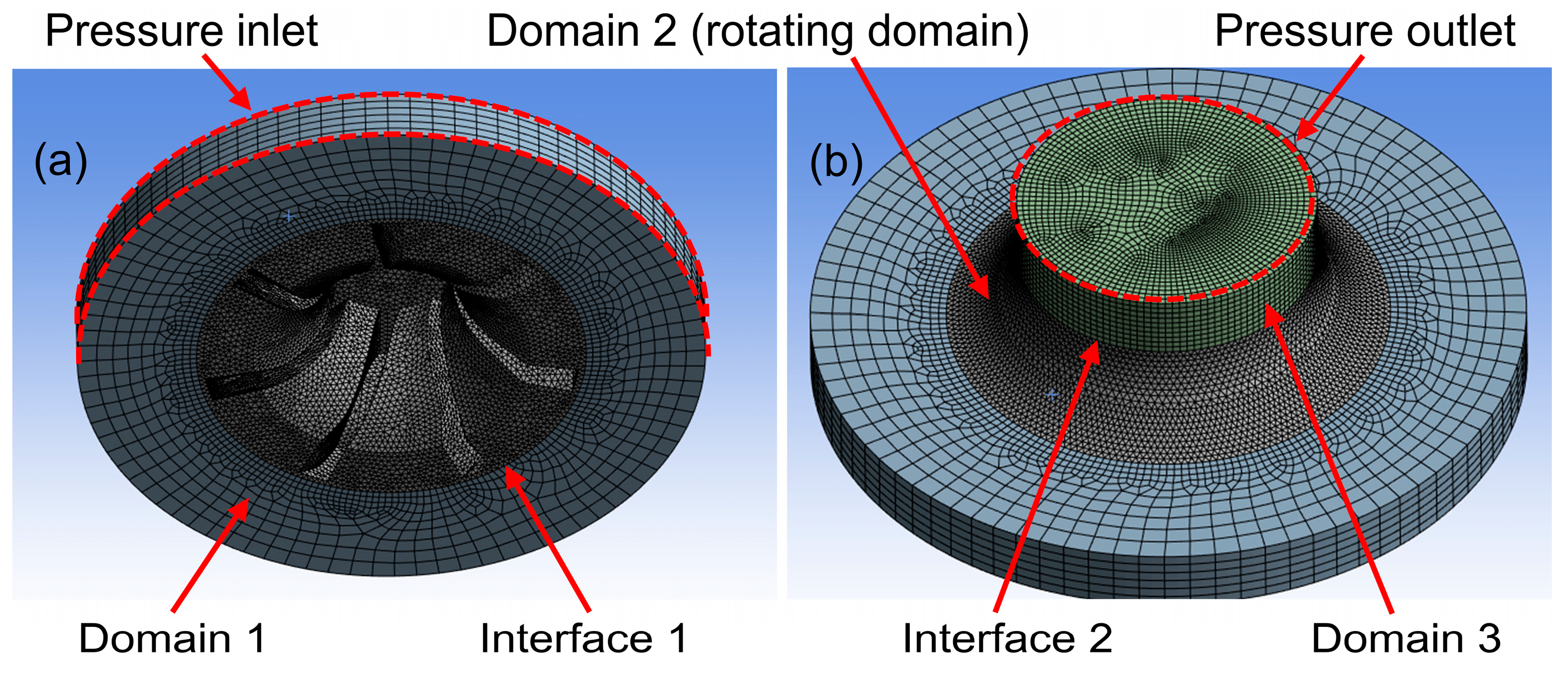
To this end, CFD simulations (Fluent 17.2, Ansys, Inc., Canonsburg, PA, USA)) are first employed to model the aerodynamic behavior of turbines with varying geometries. This approach allows for the simulation of turbines with different structural configurations, with the results of initial samples compared against experimental data to validate the accuracy of the simulations. Based on this approach, this paper employs a fully three-dimensional numerical simulation method to establish a quantitative relationship between the blade shape parameters and turbine aerodynamic performance. CFD simulations are conducted to analyze the internal flow and aerodynamic behavior of the micro-turbine under high-pressure gas drive. Figure 7 illustrates the grid division scheme and computational domain setup of the simulation model.
Figure 7.
Computational mesh and boundary condition setup for the turbine CFD model: (a) Bottom view (b) Top view.
To visually analyze the gas flow conditions at the turbine inlet and outlet, corresponding regions are extended at both the inlet and outlet positions. Therefore, the computational model consists of three key regions:
Domain 1: The upstream stagnant air region;
Domain 3: The downstream stagnant air region;
Together, these two domains form the main flow channel.
Domain 2: The rotating region containing all the turbine blades, where the rotating motion is handled using a multiple reference frame approach.
To improve computational accuracy and efficiency, the overall model uses a tetrahedral mesh for discretization. A local mesh refinement is applied to the rotating region (Domain 2), where the geometry is complex and the flow gradients are significant. The average mesh size in this region is 5 × 10⁻⁵ m to accurately capture the flow details near the blades. The turbulence model used is the RNG (Re-Normalization Group) k-ε model to ensure adaptability to low Reynolds numbers at small scales. For the turbine inlet, a pressure inlet condition is applied. For the turbine outlet, a pressure outlet condition is used, with a pressure of 0 atm. The rotational speed of the rotating domain is set to 10,000 rpm.
2.5. PINN Training Based on Active Learning
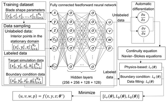
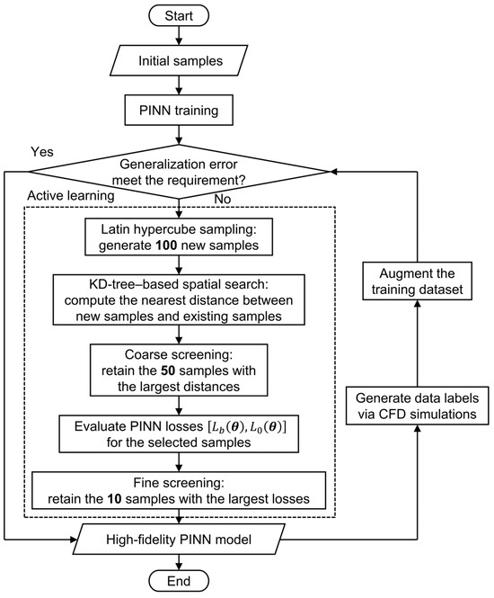
While CFD simulations provide a high-precision mapping between blade parameters and aerodynamic performance in the virtual domain, the optimization work targets a 22-dimensional design space, which requires a large number of different samples for comparative analysis. The computational cost of conducting CFD simulations for each sample in such a high-dimensional space is prohibitively high. Therefore, to enable efficient optimization, it is necessary to develop a fast and high-fidelity surrogate model for performance prediction. Based on the simulation results of the initial samples, this paper further constructs a PINN model, as shown in Figure 8, to establish a surrogate model that accurately captures the relationship between blade shape parameters and the flow field state. This model integrates both data-driven and physics-based constraints, facilitating efficient and reliable predictions of the impeller’s performance. The model construction and training process are as follows:
Figure 8.
Architecture of the PINN.
First, the initial simulation flow field data obtained under different blade shape parameter combinations are organized into a training dataset of size Nt. For any sample i with a specific set of blade shape parameters [c0, c1, c2, …, c21], spatial coordinate points and their corresponding flow field data within its computational domain are systematically collected as input-output pairs. These data are then input into a multi-layer fully connected feedforward neural network, structured as shown in the middle of Figure 8. The network consists of an input layer, multiple hidden layers, and an output layer.
During the training process, the output data is categorized into unlabeled data and labeled data, and a composite loss function is constructed accordingly:
1. Physics Equation Loss (Lr): For the unlabeled data points, the network’s predicted results are automatically differentiated to compute the residuals of the fluid dynamics governing equations (continuity equation and Navier–Stokes equations).
2. Boundary Condition Loss (Lb) and Data Fitting Loss (L0): For the labeled data, the network’s predicted values are compared with the predefined physical boundary conditions and high-fidelity simulation results. This comparison yields the boundary condition loss and data fitting loss, ensuring that the model satisfies physical constraints in key regions and fits the known data.
The network weights are iteratively updated using a gradient descent optimization algorithm to minimize the weighted sum of the three losses mentioned above.
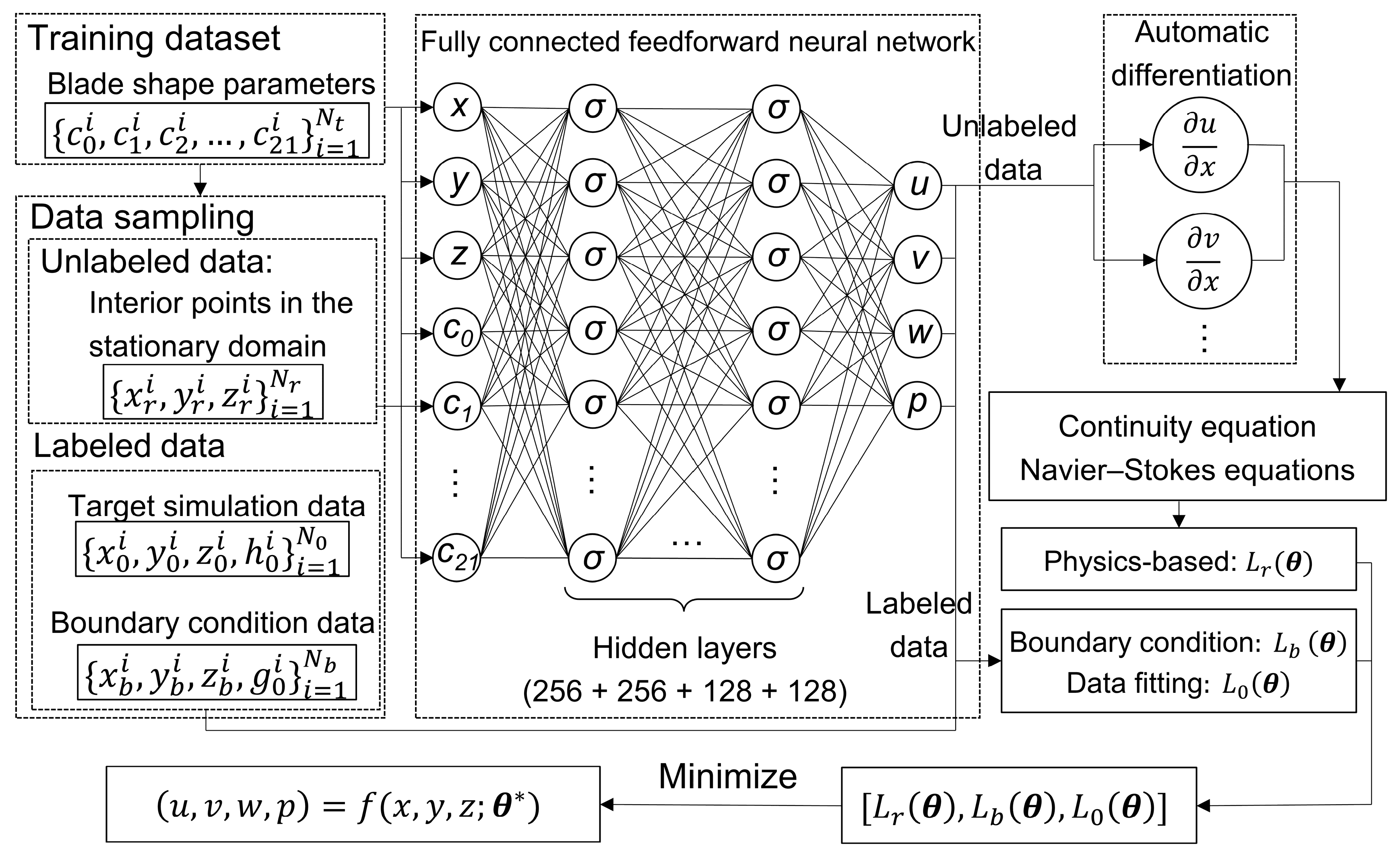
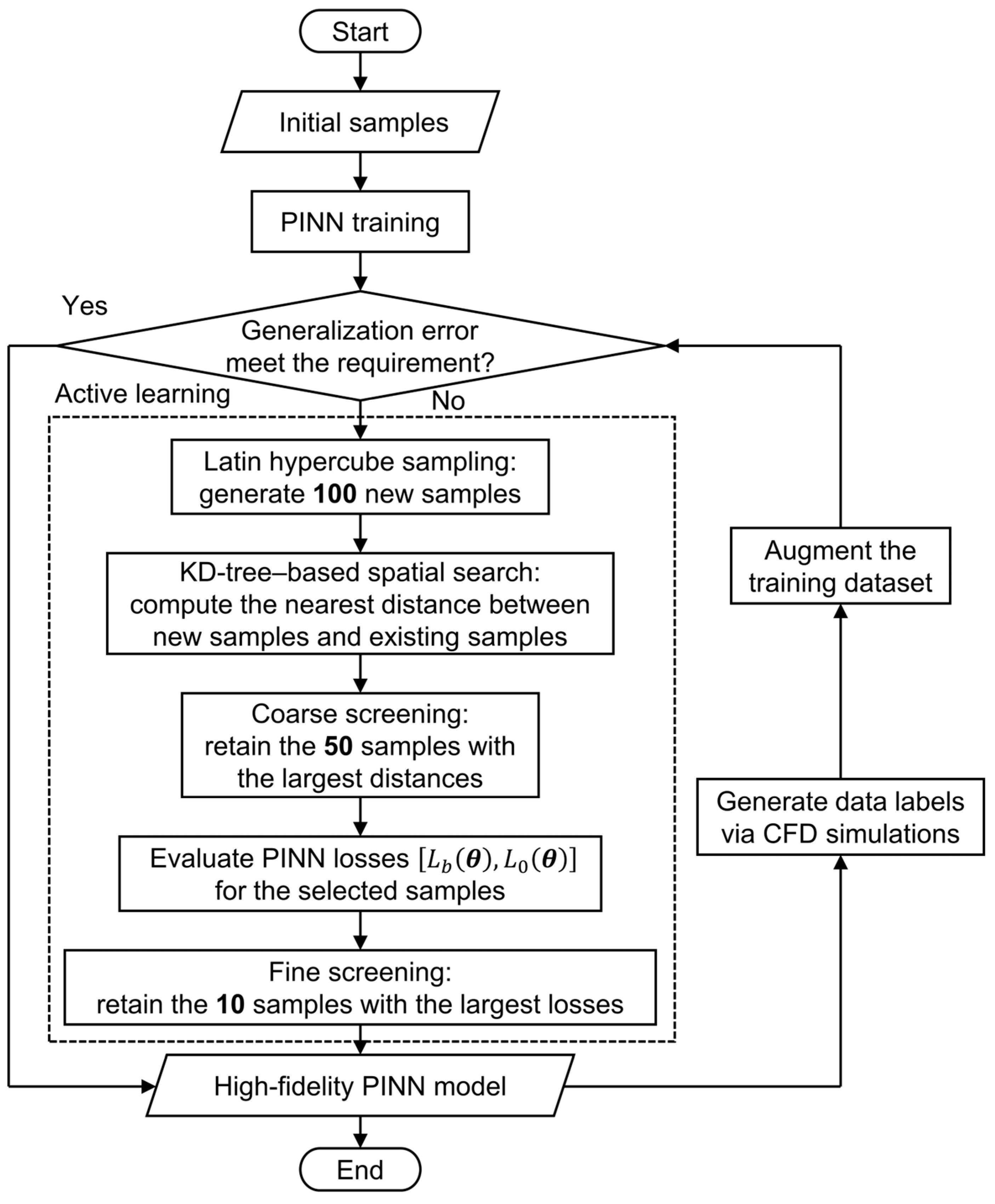
Due to the limited size of the initial sample set, the PINN model cannot achieve sufficient prediction accuracy for the mapping from blade shape parameters to the optimization objectives. To address this, additional turbine models with varied geometries need to be simulated and their results incorporated into the training set. However, conducting CFD simulations for all possible samples in the 22-dimensional design space would incur prohibitively high computational costs. Moreover, purely random sampling often results in poor coverage and low efficiency, failing to adequately explore critical regions of the parameter space. To overcome these challenges, this paper adopts the active learning framework shown in Figure 9, which enables efficient and targeted expansion of the training sample set.
Figure 9.
Sample enrichment process based on active learning.
The entire process begins with training the PINN model based on the initial sample set. The model’s generalization error is first evaluated on the validation set. If the preset accuracy requirement is not met, the active learning sample expansion module is activated. This module starts by using Latin hypercube sampling to uniformly generate 100 candidate new samples within the 22-dimensional design space, ensuring basic spatial filling of the new samples.
To select the most effective samples for model improvement, a two-stage screening strategy is employed:
1. Coarse Screening: Based on the KD-tree spatial index algorithm, the nearest neighbor distances between each new candidate sample and the existing training sample set are computed. The 50 samples with the largest distances are retained. This stage prioritizes exploring regions of the parameter space that are insufficiently covered by the existing samples, improving the diversity and coverage of the sample set.
2. Fine Screening: The 50 selected candidate samples are then input into the current PINN model. Through forward propagation, their physical residual loss and boundary condition loss are calculated. The magnitude of these losses directly reflects the model’s underfitting at those sample parameters. The top 10 samples with the highest loss values are selected for CFD numerical simulations to generate accurate flow field data labels.
Subsequently, these 10 new labeled samples are added to the original training set, and the PINN model is retrained. This process continues iteratively, efficiently expanding the training sample set until the generalization error converges to meet the requirement.
2.6. Multi-Objective Optimization
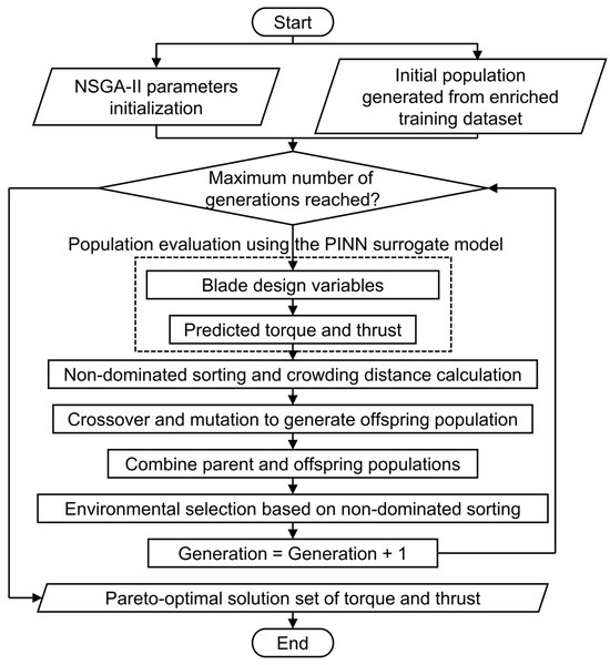
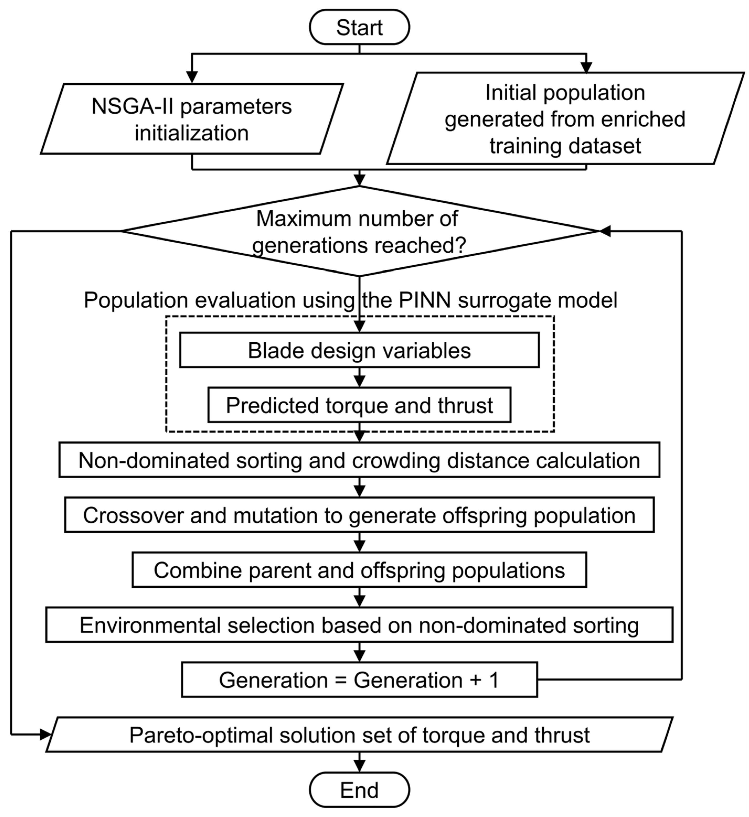
After constructing the high-precision PINN surrogate model, this paper further establishes the multi-objective blade shape optimization framework based on the Non-dominated Sorting Genetic Algorithm II (NSGA-II), as shown in Figure 10. The optimization problem is defined with three key elements:
Figure 10.
Multi-objective blade shape optimization framework based on the high-fidelity PINN surrogate model and NSGA-II.
Optimization Objectives: The optimization aims to simultaneously maximize two performance indicators: the torque exerted on the micro-turbine shaft, which reflects its rotational performance, and the axial thrust experienced by the turbine, which characterizes its contribution to MAV’s propulsion.
Design Variables: The 22 blade geometry parameters defined in Section 2.2, [c0, c1, …, c21], serve as the design variables. All variables are normalized to the range [0, 1] to facilitate optimization.
Constraints: Geometric constraints derived in Section 2.1 and Section 2.2, based on manufacturing limitations and turbine geometry, are imposed. These include the number of blades (5 ≤ N ≤ 15) and blade thickness (t ≥ 0.1 mm). The normalized design variable range [0, 1] ensures that all constraints are inherently satisfied.
The expanded training sample set is used as the initial population. The NSGA-II algorithm parameters are initialized first, including population size, crossover probability, mutation probability, and the maximum number of iterations. In each generation of the iteration process, the torque and thrust for each individual are first calculated based on the PINN prediction results. Non-dominated sorting and crowding distance calculations are performed to evaluate the quality and uniformity of the solution distribution. Then, crossover and mutation operations are applied to generate the offspring population, and both the parent and offspring populations are combined. An environmental selection strategy based on non-dominated sorting is used to select the new generation population. This process continues iteratively until the termination condition is met.
Finally, a Pareto-optimal solution set of torque and thrust is obtained, providing the optimal design solutions under a multi-objective trade-off for turbine blade design.
3. Results and Discussion
This section systematically verifies the proposed intelligent design framework for 3 mm-diameter micro-turbine blades, focusing on rotational speed and thrust performance. Starting from micro-fabrication and aerodynamic testing of the initial samples, experimental benchmarks were established to validate subsequent numerical models. Guided by these results, 3D CFD simulations were conducted to create a low-cost virtual mapping between blade parameters and turbine performance. Based on this, a PINN surrogate model was trained using a two-stage active learning strategy, enabling efficient dataset expansion and improved prediction accuracy. The trained PINN was then employed as the objective function in a multi-objective optimization using the NSGA-II algorithm to obtain a Pareto-optimal solution set reflecting the inherent trade-offs. Finally, the optimized samples were validated through micro-fabrication and aerodynamic testing, completing the full design loop.
3.1. Experimental Performance Testing for Initial Samples
The key to designing micro-turbine blades lies in establishing a mapping relationship between the geometric parameters and aerodynamic performance, allowing for the comparison of different configurations and the selection of optimal designs. Therefore, this section begins with physical testing, where actual micro-turbine prototypes with varying geometries are fabricated and their performance data are measured. Given the high cost of physical testing, only a limited number of samples can be tested. However, these experimental results provide the most accurate data, serving as an essential reference for the subsequent development of the mapping relationship in the virtual domain.
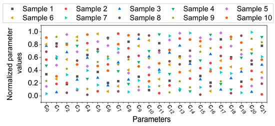
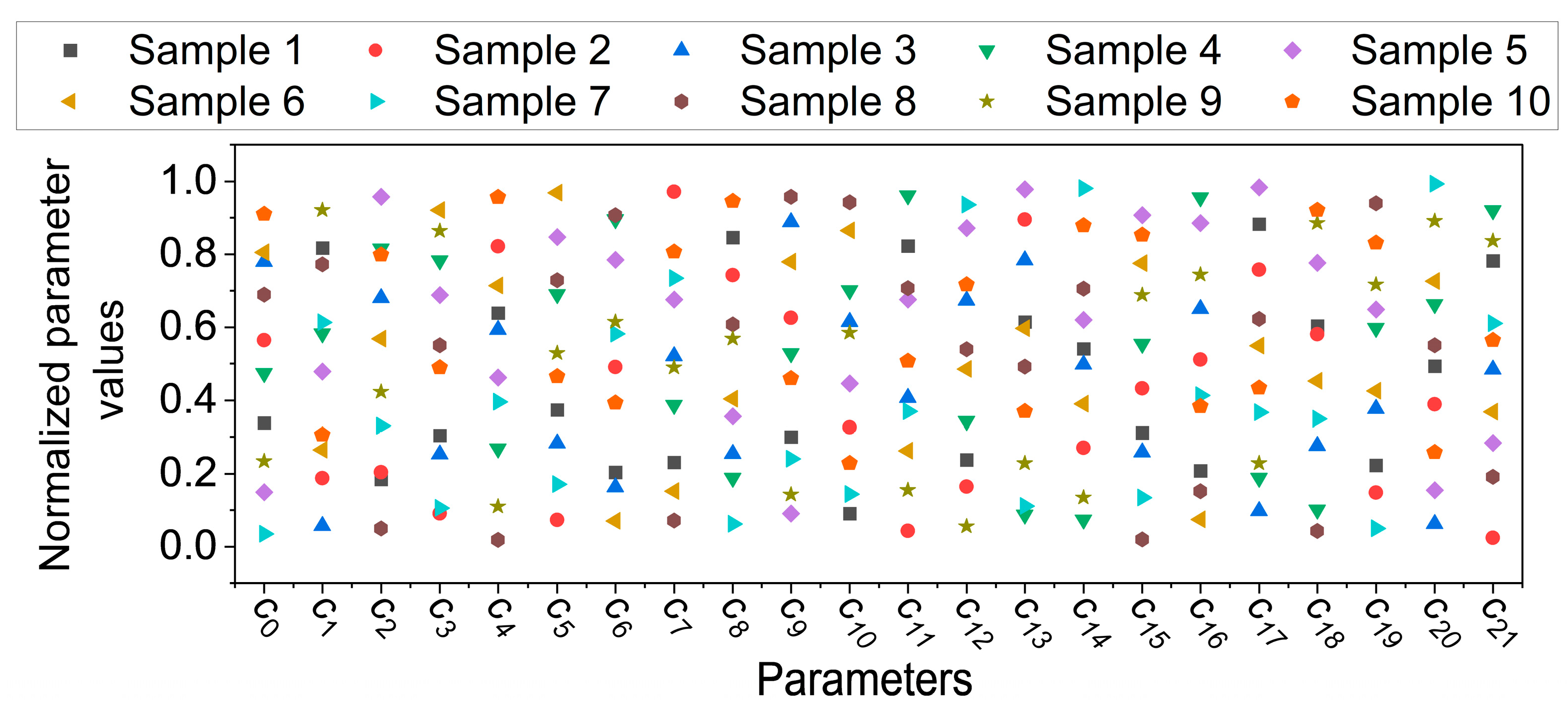
To ensure the uniform coverage of the initial samples across the parameter space, this paper uses the LHS method to generate 10 initial samples. Figure 11 shows the distribution of the initial samples across different blade shape parameter dimensions, with all parameters normalized to the range [0, 1]. It can be observed that the samples exhibit good dispersion across each parameter dimension, without any obvious clustering or gaps. This indicates that the LHS method effectively avoids the issue of concentrated sample distribution in the high-dimensional parameter space. The uniform and random sample distribution provides a reliable initial foundation for the subsequent PINN model training and active learning sample expansion process. The physical definition and design constraints of the 22 blade geometry parameters (c0–c21) used for sampling are detailed in Table 1, which correspond to the blade profile parametric modeling process described in Section 2.2 and Figure 4.
Figure 11.
Distribution of the initial samples across different parameters.
Table 1.
Definition and constraints of the 22-blade geometry parameters.
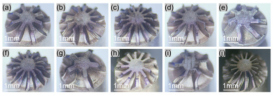
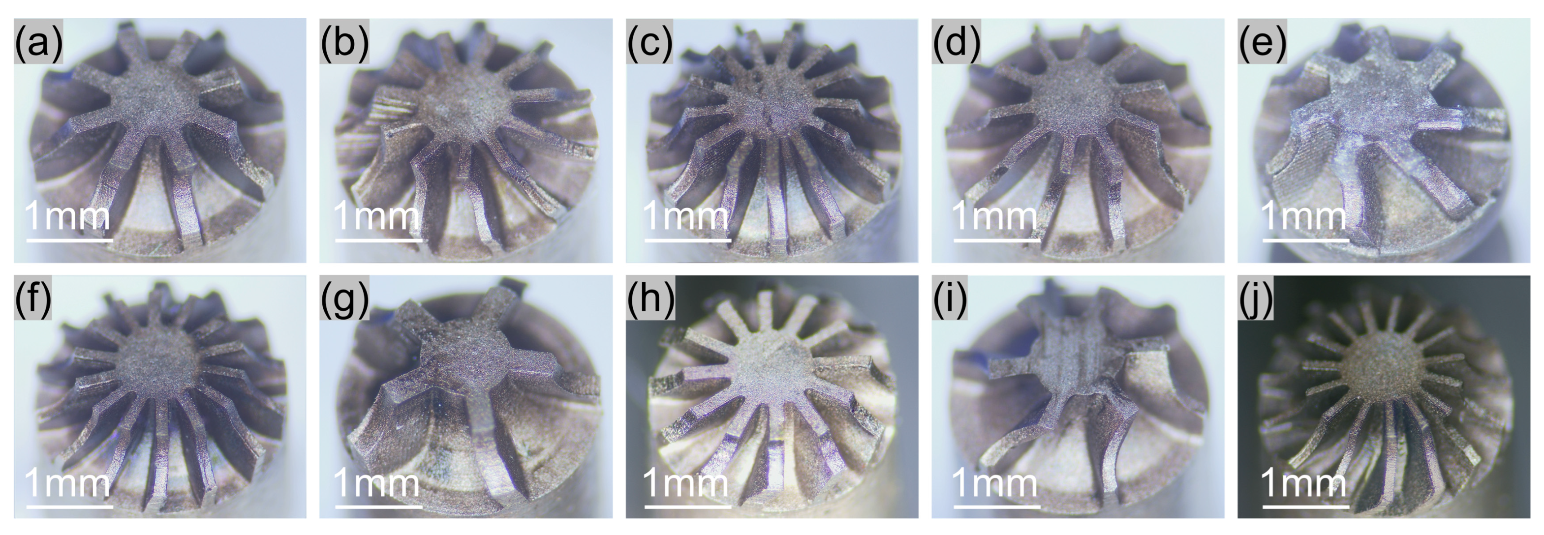
Figure 12 shows the manufacturing results of the 10 micro-turbine samples, each corresponding to different initial samples. The blade shapes exhibit significant morphological differences, further confirming that the sampling method, as shown in Figure 11, provides broad coverage of the parameter space. Despite the strong randomness in the parameter combinations, each sample corresponds to a well-defined turbine structure, and all fabrication processes were successfully completed. This demonstrates the robustness of the blade morphology parameterization method based on manufacturing feasibility: it not only enables the generation of diverse blade shapes but also ensures that all designs meet the required manufacturing conditions. These manufacturing results enable the possibility of performance testing on micro-turbines in a real physical context, serving as the basis for obtaining the most accurate representation of the turbine’s true operating conditions.
Figure 12.
Manufacturing results of the micro-turbines corresponding to the initial samples: (a) Sample 1: 8 blades, thickness 0.187 mm; (b) Sample 2: 11 blades, thickness 0.100 mm; (c) Sample 3: 13 blades, thickness 0.116 mm; (d) Sample 4: 10 blades, thickness 0.129 mm; (e) Sample 5: 7 blades, thickness 0.152 mm; (f) Sample 6: 14 blades, thickness 0.112 mm; (g) Sample 7: 5 blades, thickness 0.222 mm; (h) Sample 8: 12 blades, thickness 0.131 mm; (i) Sample 9: 6 blades, thickness 0.110 mm; (j) Sample 10: 15 blades, thickness 0.101 mm.
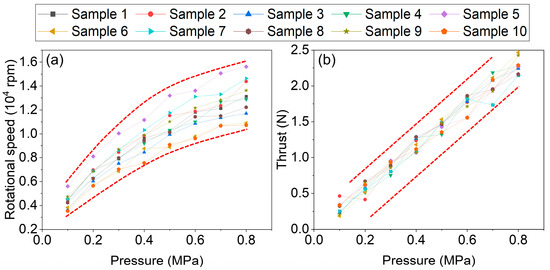
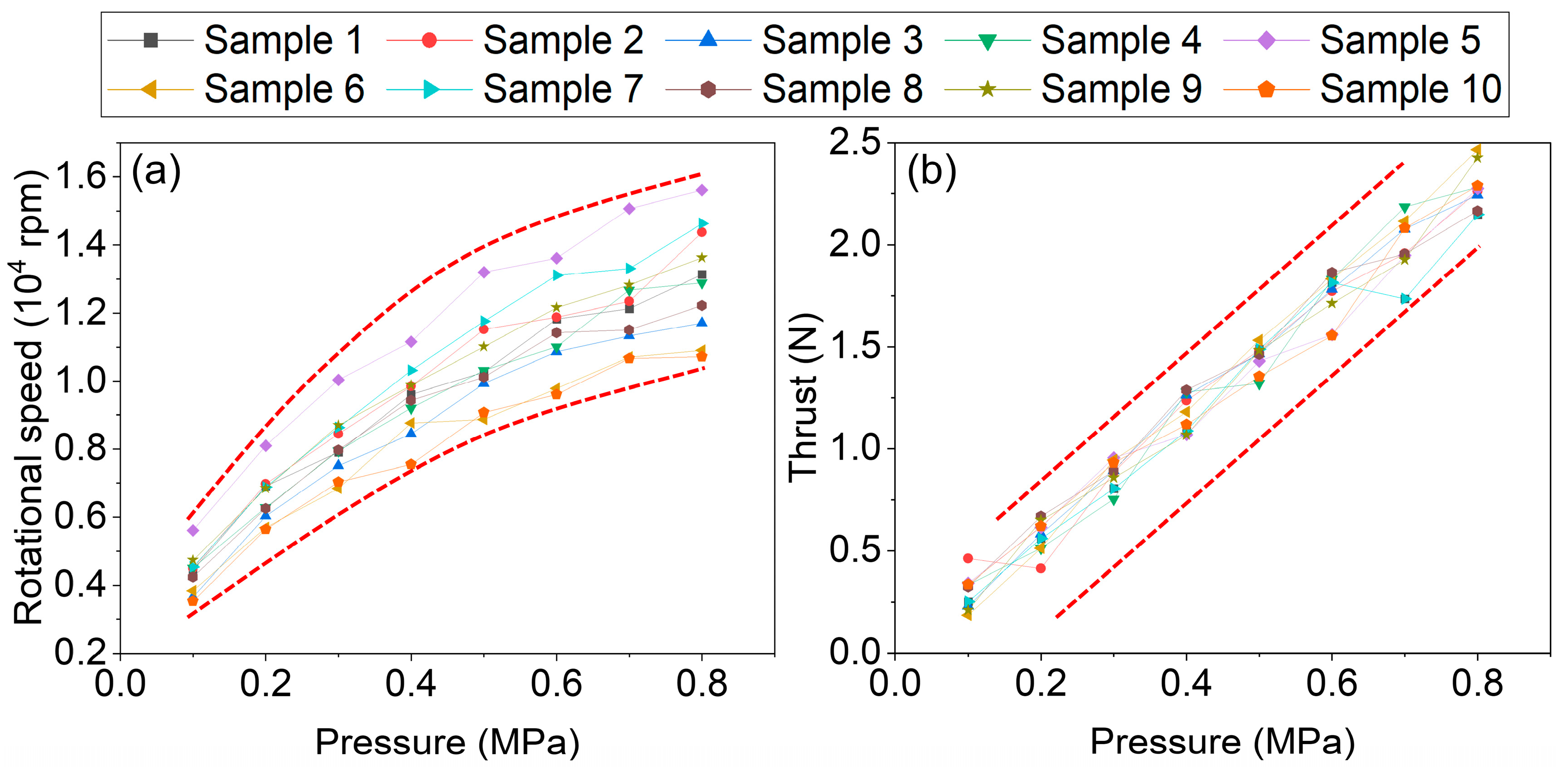
After fabricating the physical prototypes of the initial samples, they were installed on the test platform shown in Figure 6 to measure two fundamental performance metrics: rotational speed and thrust. To ensure broad coverage of operating conditions and facilitate comparison with subsequent simulation results, full-range tests were conducted under varying intake pressures from 0.1 to 0.8 MPa. The results are presented in Figure 13. From the rotational speed results in Figure 13a, it can be observed that during the low-pressure phase (when intake pressure is below 0.5 MPa), the rotational speed increases rapidly with the rise in pressure, indicating that the increase in energy input is effectively converted into the rotor’s kinetic energy. Once the pressure exceeds 0.5 MPa, the growth rate of the rotational speed significantly slows, and the overall trend shows a rapid rise followed by saturation, which is attributed to factors such as increased gas leakage and higher flow losses at higher pressures. Moreover, there are significant performance differences between the various samples. For example, Sample 5 maintains the highest rotational speed at all test pressures, while Sample 10 has the lowest rotational speed under most conditions. This directly reflects the critical influence of the blade morphology on the turbine’s aerodynamic performance, demonstrating the practical necessity and potential for performance improvement through blade shape optimization. As shown in Figure 13b, the thrust variation trend for the same turbine sample is more complex. However, the overall trend indicates a linear increase in thrust with rising intake pressure. This section provides a full-pressure-range characterization of the turbines’ target performance, yielding high-fidelity data and trends that serve as an essential reference for evaluating and validating subsequent CFD simulation results.
Figure 13.
Initial sample test results: (a) Rotational speed and (b) thrust under different air pressures.
3.2. Analysis and Verification of CFD Simulation Results
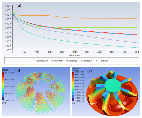
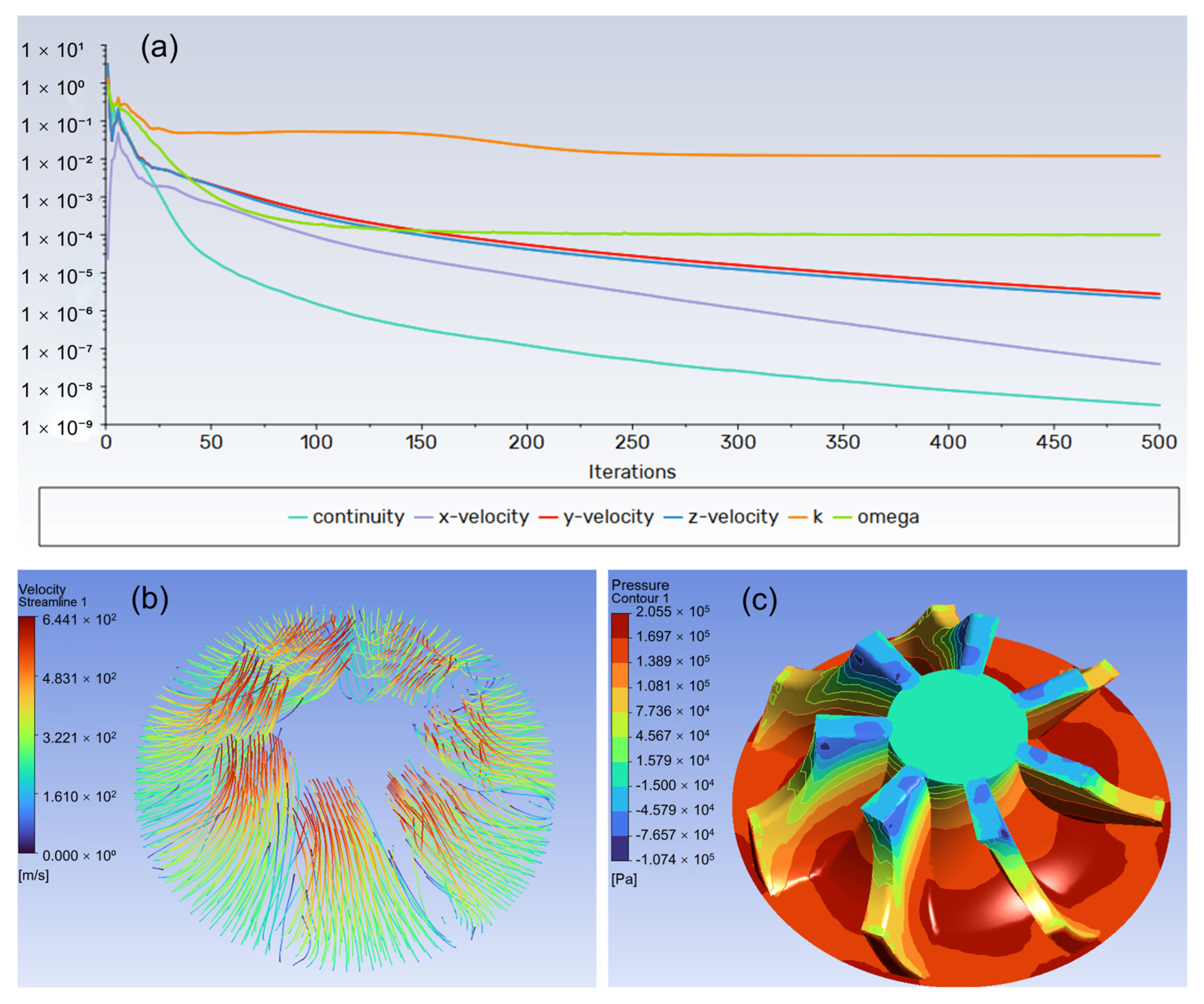
The initial experimental study provided preliminary measurements of the rotational speed and thrust performance for a small sample of blade designs, establishing a physical relationship between the blade structure and its operating performance at a practical scale. However, due to the high fabrication costs associated with physical testing, it was not feasible to cover a large number of samples. For a 22-dimensional parameter space, the 10 available experimental samples are far too few to meet the data requirements for neural network training. Therefore, this study further employs CFD simulations to evaluate the performance of micro-turbines with different blade morphologies. The aim is to establish a broader correlation between turbine blade parameters and aerodynamic performance at a lower cost, across a more extensive sample space. In this way, CFD simulations can be used to evaluate a much larger set of samples, generating the mapping between blade morphology parameters and performance results, which serves as a training set for developing a high-accuracy surrogate model. Specifically, CFD simulations were first conducted on the initial samples shown in Figure 12, with the key results from the simulation of sample 5 (Figure 12e) presented in Figure 14.
Figure 14.
CFD simulation results of the micro-turbine: (a) Residual curves. (b) Flow field in the rotating region. (c) Pressure distribution on the blade surface.
Figure 14a presents the residuals curve, where it can be seen that the residuals of all physical quantities decrease rapidly with the number of iterations and eventually fall below the set convergence criterion, indicating that the numerical calculation has reached a stable and reliable solution. Figure 14b shows the flow trajectories of the working fluid in the rotating region. Under low Reynolds number flow conditions, the gas streamlines follow the blade surface well, with no large-scale vortices or flow separation occurring. This is beneficial for reducing flow losses and improving energy conversion efficiency. Figure 14c further provides the static pressure distribution contour on the blade surface. When the high-pressure gas flows radially in, the pressure in the blade cup is significantly higher than on the blade surface, forming a stable pressure difference on both sides of the blade. This pressure difference provides an effective driving torque for the rotor shaft, which is the core aerodynamic force that drives the micro-turbine to rotate continuously in a counterclockwise direction. These simulation results clearly reveal the internal flow characteristics and work mechanism of the micro-turbine under the given operating conditions from both the flow field structure and blade load perspectives. The above results preliminarily demonstrate that the established simulation process is capable of achieving stable, convergent calculations for the micro-turbine’s working flow field. Additionally, the flow field state depicted by the results provides a theoretical foundation for the effective operation of the micro-turbine. Building on this, for different initial samples, we now need to extract the simulation results related to rotational speed and thrust, and compare them with the experimental data. This will allow us to specifically examine the correspondence between blade parameters and performance outcomes.
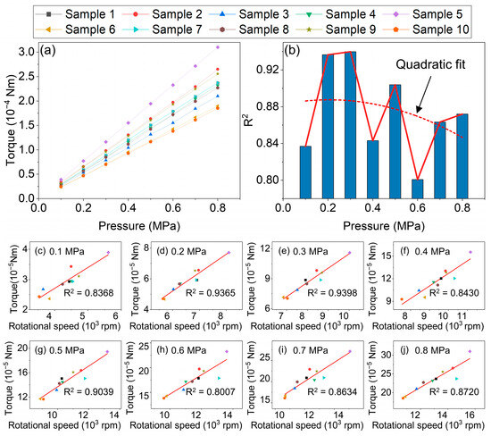
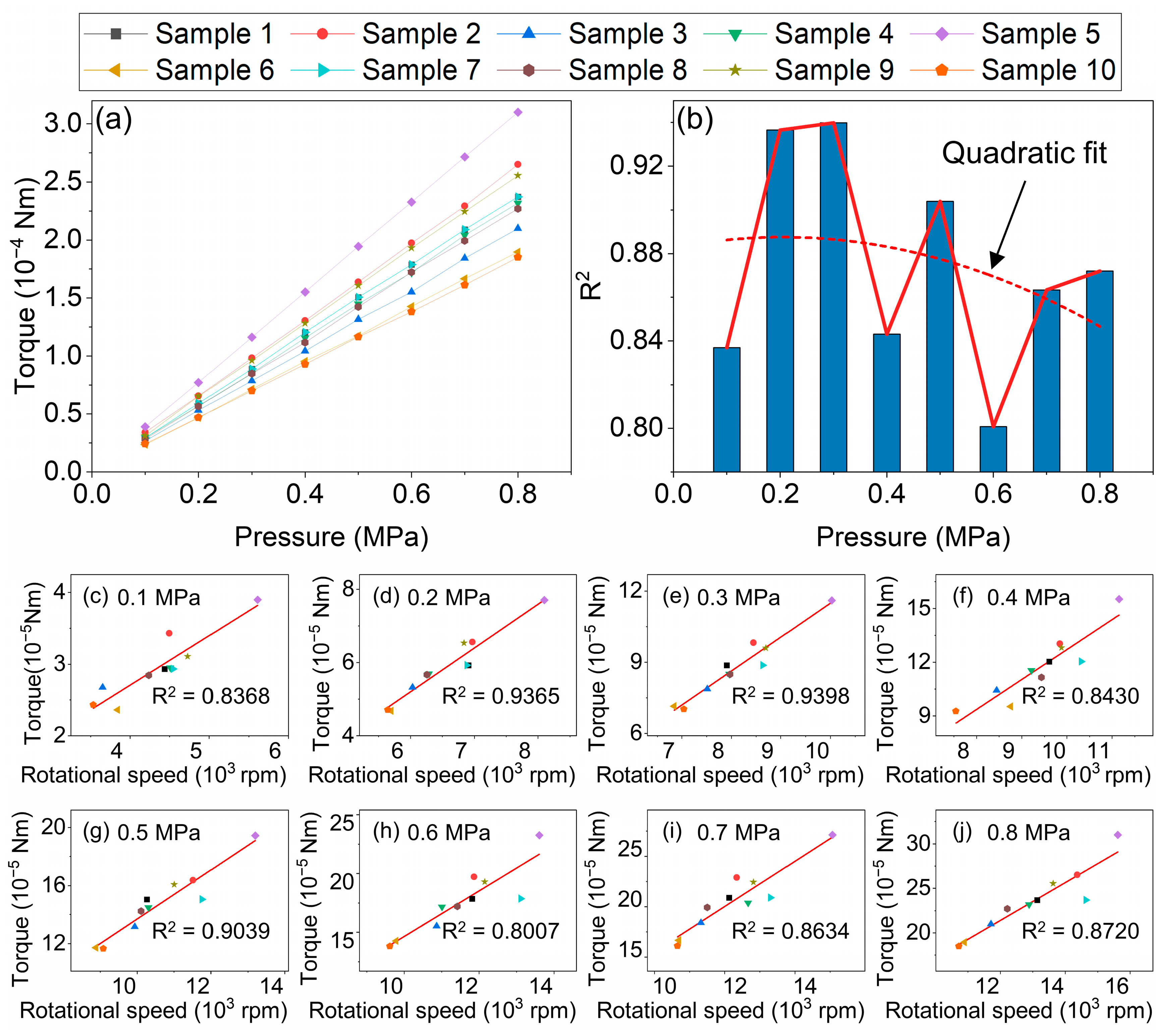
Figure 15 shows the simulation torque of the initial samples under different pressure conditions and its correlation with the experimental rotational speed. From Figure 15a, it can be observed that as the pressure increases, the torque increases approximately linearly, with samples having initially low torque showing a lower rate of increase. This indicates that the torque data for each sample does not cross over. From Figure 15c–j, it is evident that the torque is strongly correlated with the experimental rotational speed, with the correlation coefficient R2 generally higher than 0.8. This strongly confirms that the simulated torque and experimental rotational speed data are highly correlated and can be used as a surrogate indicator for assessing turbine rotational speed performance at the simulation method. The summary of R2 values in Figure 15b shows that as the pressure increases, the complex effects of experimental factors such as leakage gradually become more significant, leading to a decrease in the correlation between torque and rotational speed. At low pressure (0.1 MPa), the relative fluctuations in the measurement results due to experimental system errors also affect the correlation. Therefore, the simulated torque under the condition of 0.2 MPa most accurately reflects the relationship with the rotational speed. Considering the pattern of the simulated torque data (linear and non-crossing), the torque relationships at different samples under the same pressure can be approximated to reflect the torque relationships across all pressure conditions. Thus, under the 0.2 MPa condition, the relative ranking of simulated torque for different samples can be used to infer their rotational speed performance ranking across the entire pressure range, providing a basis for subsequent sample selection in simulations.
Figure 15.
Torque simulation and correlation analysis under different air pressures: (a) Torque of 10 initial samples under different pressures. (b) Summary of correlation coefficients R2 between simulated torque and experimental rotational speed. (c–j) Torque vs. rotational speed under 0.1–0.8 MPa.
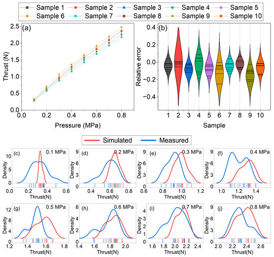
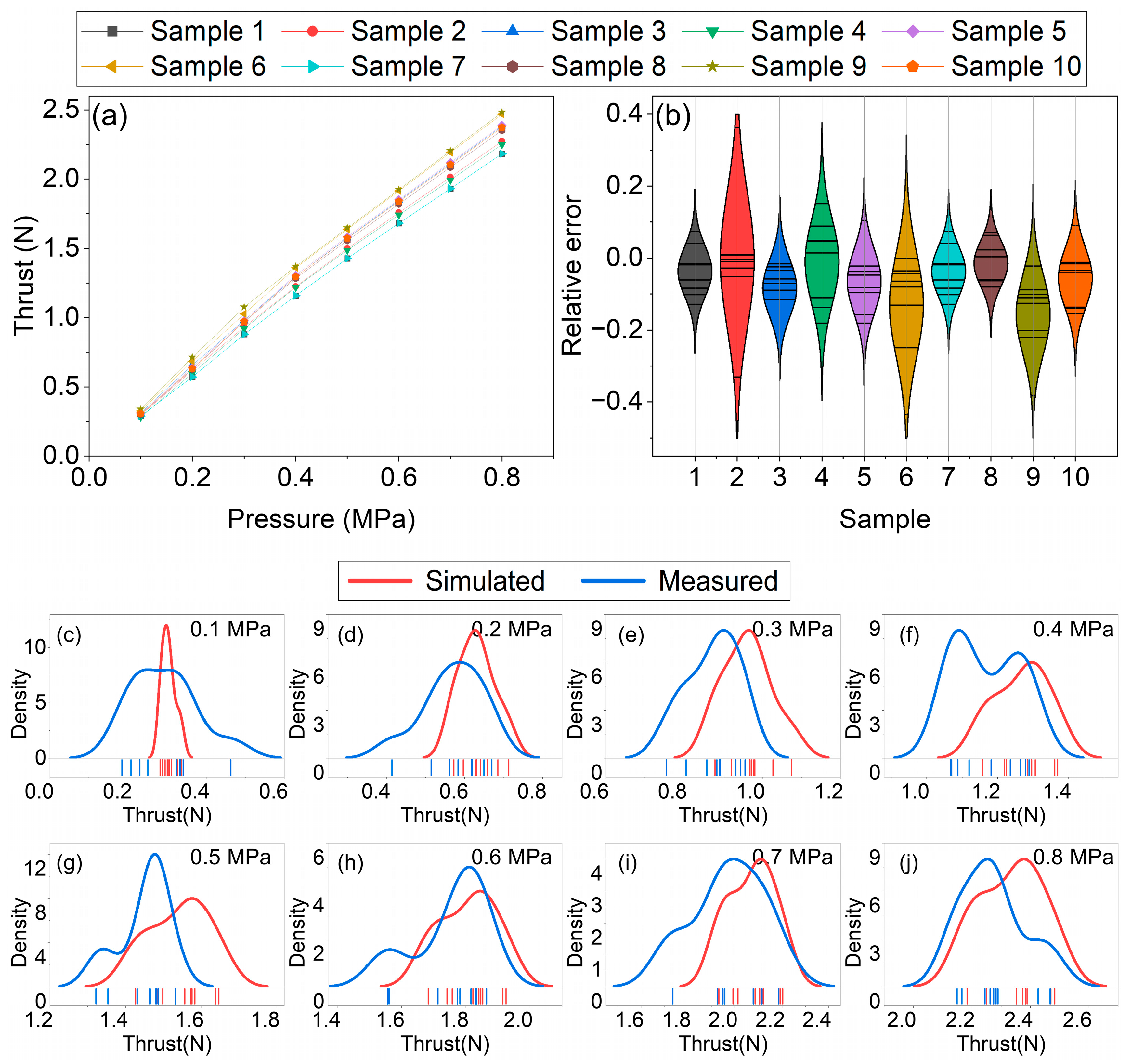
Figure 16 presents a comparative analysis of simulated thrust and test results under different inlet pressure conditions. Figure 16a shows that for Samples 1~10, the simulated thrust increases approximately linearly with pressure, which aligns with the experimental observations in Figure 13b. Figure 16b presents the distribution of relative errors between the simulated and measured thrust values for each sample using a box plot. The results show that the majority of the errors are controlled within 20%, with most errors concentrated in the 0~10% range (the median is approximately 6.73%), confirming the overall effectiveness of the simulation model in estimating thrust. Figure 16c–j further reveals the dynamic variation in error with pressure. At the low pressure of 0.1 MPa, the measured data are significantly affected by system noise, leading to a wide distribution and large error. As the pressure increases to 0.2 MPa and above, the probability density distributions of the simulated and measured data converge rapidly, with a high degree of agreement and a significant reduction in error. Based on this, and to maintain consistency with the torque simulation conditions, this study selects 0.2 MPa as the standard inlet condition for subsequent thrust performance comparison and evaluation, ensuring that the analysis results are based on the minimum error and highest consistency.
Figure 16.
Simulation and test results of thrust under different air pressures: (a) Simulated thrust of 10 initial samples under different pressures. (b) Distribution of relative error between simulated and measured thrust for different samples. (c–j) Distribution of simulated and measured thrust at pressures of 0.1–0.8 MPa.
The analysis of the simulation results for the initial samples has validated the reliability of the simulation method for modeling the turbine flow field. Furthermore, by extracting key data and comparing it with experimental results, it was confirmed that under the 0.2 MPa intake pressure condition, the simulated torque and thrust data most accurately correspond to the turbine’s actual rotational speed and thrust performance. This conclusion lays the foundation for the establishment of the training set. For subsequent simulations of additional samples, it is sufficient to perform simulations only under the 0.2 MPa intake condition, using the resulting torque and thrust data as a comparative basis for the performance of turbines with different structures. This approach eliminates the need for full-pressure-range simulations for each sample, significantly reducing the cost of data accumulation.
3.3. Establishment of PINN and Analysis of Parameter Influence
The training of a PINN requires a large number of samples linking parameters with performance as the training dataset. Based on the above research, it is evident that CFD simulations can achieve this goal at a relatively low cost. However, the computational resources consumed by significantly increasing the number of CFD samples inherently limit the size of the training dataset. Therefore, to achieve the desired training effect with a limited dataset, it is crucial to carefully select the parameter distribution of the training samples to ensure their contribution to the PINN model training is maximized. To address this challenge, this section employs the active learning approach shown in Figure 9 to gradually expand the training set in batches.
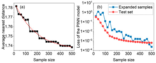
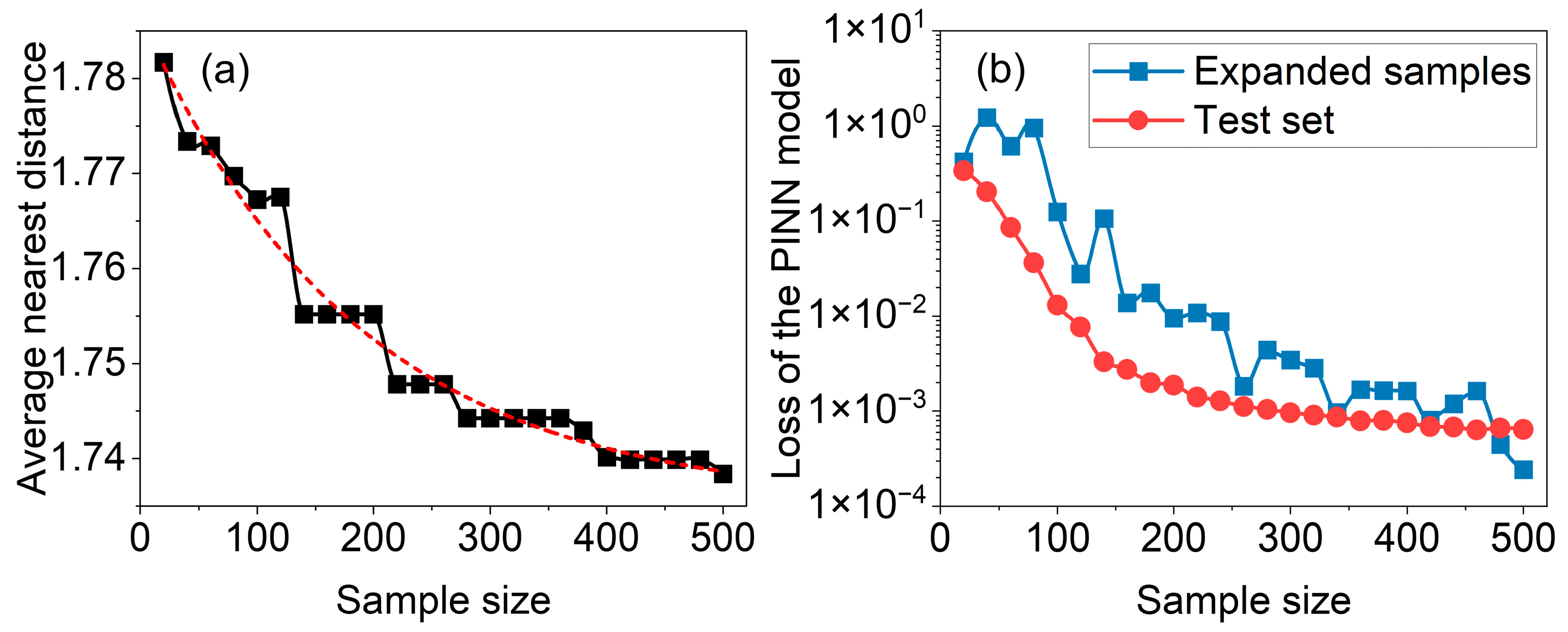
Figure 17 illustrates the impact of gradually increasing the training sample size on both parameter space coverage and the prediction performance of the PINN model within an active learning framework. Figure 17a reflects the evolution of the distribution of training samples in the design space. As the sample size increases, the average nearest neighbor distance between samples continuously decreases, indicating that the newly added samples effectively fill the gaps in the high-dimensional parameter space, improving both the representativeness and spatial uniformity of the sample set. When the sample size reaches around 500, the rate of decrease in the average distance slows down significantly, suggesting that the main regions of the parameter space have been adequately sampled, and further increasing the sample size leads to diminishing returns in terms of spatial coverage improvement.
Figure 17.
Analysis of the impact of sample size on parameter space coverage and PINN model performance: (a) Evolution of average nearest distance between samples with increasing sample size. (b) Loss variation in the PINN model during sample expansion.
Figure 17b concurrently records the loss variation in the PINN model during the sample expansion process, revealing the evolution of the model’s learning and generalization abilities. The blue curve represents the average physical loss calculated by the PINN for the candidate samples selected in each round of active learning. This loss steadily decreases as the sample size increases, indicating that the model continually strengthens its internal understanding of physical laws through the incorporation of new samples, thereby enhancing its prediction capability for unknown parameter points. The red curve represents the total loss evaluated on an independent test set, providing a more comprehensive reflection of the model’s overall generalization performance. When the sample size reaches around 500, the test set loss drops below 1 × 10⁻³ and the subsequent decrease becomes relatively flat, indicating that the model’s prediction accuracy has converged. The contribution of adding further training samples to accuracy improvement becomes limited. Based on this analysis, active learning expansion is stopped at 500 samples. At this point, the sample distribution adequately covers the key parameter space, and the PINN model achieves satisfactory predictive performance on the test set that meets engineering accuracy requirements. Finally, all high-fidelity simulation data at this sample size are integrated to fully train the PINN model and fix its network weights, resulting in a flow field surrogate model with both high accuracy and fast prediction capabilities.
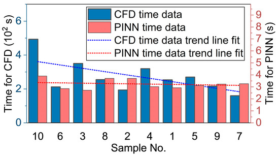
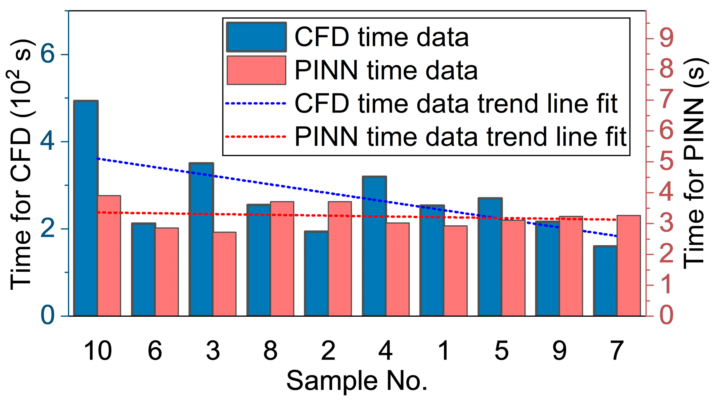
To quantitatively evaluate the computational efficiency and cost-effectiveness of the trained PINN surrogate model relative to conventional CFD methods, the single-sample computation times of both approaches were compared across all initial samples, as shown in Figure 18. The results indicate that the average computation time per sample using the CFD method is 272.3 s, whereas the trained PINN model requires only 3.2 s on average, representing an improvement of two orders of magnitude in computational efficiency. This finding highlights the significant advantage of the PINN surrogate in rapid performance prediction, providing practical feasibility for extensive parameter-space exploration, screening, and comparison. Additionally, all samples in Figure 18 are sorted by blade count in descending order. The results reveal a clear trend: CFD computation time increases markedly with blade number, as reflected in the downward-sloping linear fit, due to the higher geometric complexity and mesh density associated with additional blades, which substantially increase numerical iteration costs. In contrast, the PINN model exhibits nearly constant computation time regardless of blade number or geometric features, with a linear fit that is almost horizontal, demonstrating strong computational stability. Overall, the PINN surrogate not only dramatically reduces the time required for single-sample performance prediction but also maintains stable efficiency across varying geometries, making it highly suitable for large-scale rapid evaluation and providing a solid computational foundation for subsequent multi-objective optimization.
Figure 18.
Comparison of CFD and PINN computational time for initial samples.
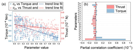
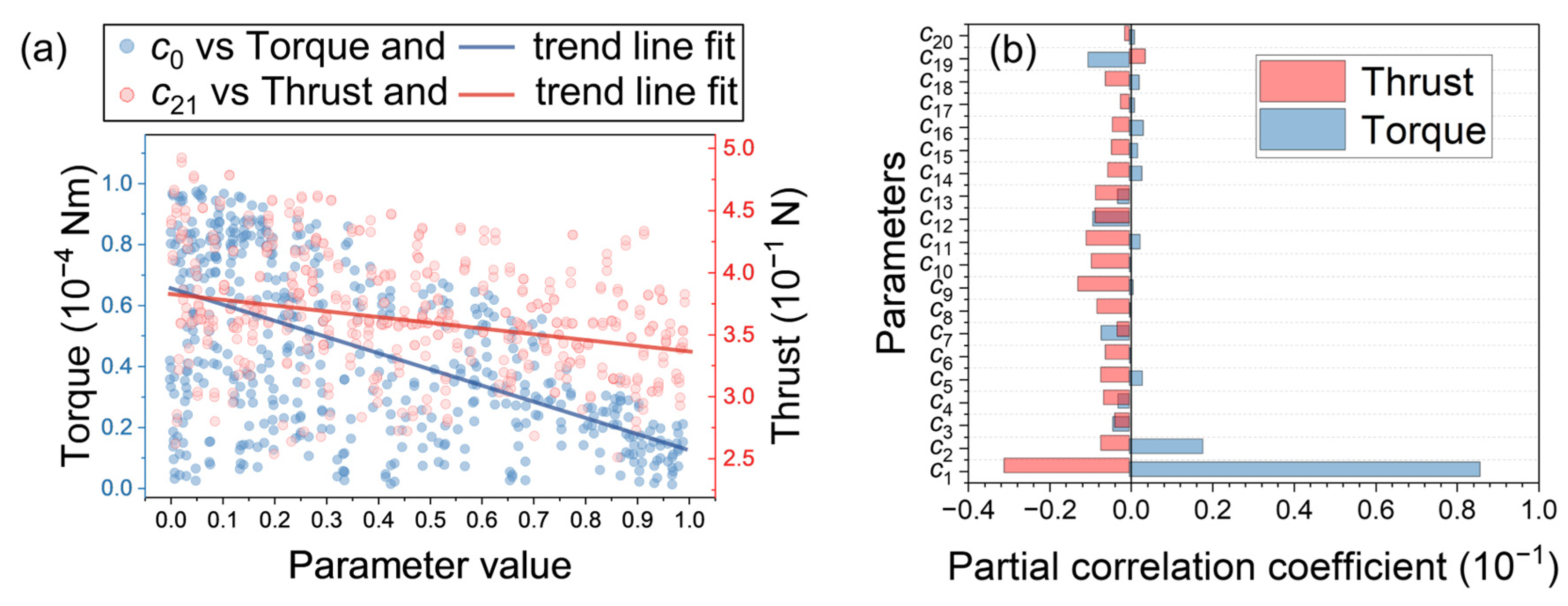
During the PINN training process with an active learning strategy, a high-quality dataset of 500 samples was generated through CFD simulations. Based on this dataset, a global sensitivity analysis of the design parameters with respect to two key performance metrics of the turbine—torque and thrust—was conducted, as shown in Figure 19. As illustrated in Figure 19a, the blade number parameter c0 exhibits the most significant effect on torque, displaying a clear negative correlation, whereas the blade thickness parameter c21 demonstrates the strongest regulatory effect on thrust, also with a negative trend. These results provide a direct illustration of the dominant influence of the two primary design variables on their respective target performances. Building on this, Figure 19b presents the partial correlation coefficients of the blade centerline shape parameters [c1~c20] with torque and thrust. It can be observed that most centerline parameters exert opposing effects on the two performances metrics: parameters contributing positively to torque often have a negative impact on thrust, and vice versa. This observation preliminarily indicates an inherent trade-off between torque and thrust in the micro-turbine, making it challenging to simultaneously enhance both through adjustment of a single parameter. Consequently, multi-objective optimization is necessary to obtain designs that achieve a balanced improvement in both performance metrics.
Figure 19.
Influence of parameters on torque and thrust: (a) Sensitivity analysis of parameters on torque and thrust (b) Partial correlation analysis of parameters about blade centerline.
Through the above work, a PINN surrogate model with considerable accuracy has been established to predict the performance corresponding to different blade input parameters [c0~c21]. This model offers computational efficiency far exceeding that of CFD simulations, enabling rapid comparison and screening across a wide range of parameter combinations. However, the parameter analysis indicates that the influence of blade parameters on turbine performance is highly complex, and there exists an inherent trade-off between the two key performance metrics, torque and thrust. This implies that simply optimizing a few individual parameters is insufficient to identify the optimal turbine structure. In addition, blindly sampling a large number of points in the 22-dimensional parameter space is inefficient for locating the optimal configuration. Therefore, it is necessary to employ a more powerful multi-objective optimization algorithm, using the mapping established by the PINN as the objective function, to systematically identify the final optimal sample.
3.4. Multi-Objective Optimization and Final Sample Validation
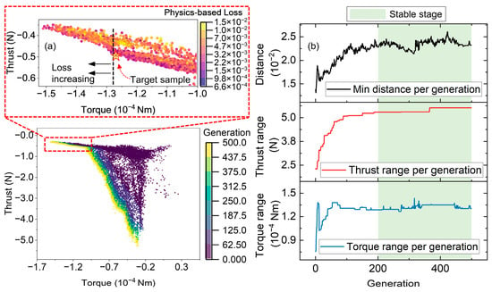
Building on the analysis from previous studies, this paper employs the NSGA-II algorithm for multi-objective optimization of torque and thrust performance using the established PINN model. The aim is to investigate the trade-off relationship between these two objectives across a broader parameter space and guide the selection of the final sample. The optimization process and results are shown in Figure 20. Figure 20a illustrates the evolution of the sample distribution in the objective space during the optimization. As the number of iterations increases, the algorithm successfully approximates and defines a continuous, smooth, and typically concave Pareto front, clearly revealing the inherent trade-off between the two objective values. The convergence trajectory of the algorithm is clearly displayed by the color gradient based on the generation index: early populations explore the objective space widely, while as evolution progresses, the solution set gradually converges and tightly clusters near the front, proving that the NSGA-II effectively balances global exploration and local exploitation. The solution set is evenly distributed along the Pareto front, with no significant clustering or sparse regions, indicating that the crowding distance mechanism maintains population diversity well.
Figure 20.
Optimization process of the micro-turbine using the NSGA-II algorithm: (a) Evolution of sample distribution and physics-based loss as the generation progresses. (b) Overall range of thrust and torque, and the minimum distance between samples per generation during the optimization process.
Since the turbine itself is made of lightweight network microstructure titanium composite materials, the thrust requirement is relatively low, and the design tends to favor achieving higher torque. Hence, we focus on the left side of the Pareto front. In the local magnified view, it can be observed that as torque further increases, the physical equation loss begins to rise significantly, indicating that this optimization front approaches the boundary of the physically feasible domain. Based on this observation, we select an optimal compromise point on the trade-off curve, just before the loss begins to rise steeply, and mark it with a star on the figure as the final recommended target sample.
To assess the convergence of the optimization process, Figure 20b shows the range of thrust and torque for each generation of the population, as well as the minimum distance between individuals in the same generation. The results indicate that after about 200 generations, the thrust range, torque range, and the minimum distance between individuals stabilize and the fluctuation significantly decreases. This suggests that the algorithm has fully explored the objective space, and no significant improvements are being made to the population, signaling that the optimization process has reached convergence. Therefore, the total iteration count of 500 generations set in this study ensures stable and converged optimization results.
In conclusion, the NSGA-II algorithm successfully provides the Pareto optimal solution set for both thrust and torque of the micro-turbine, and based on the physical equation loss, the feasible optimal design point for engineering applications is determined. The convergence analysis confirms the robustness and effectiveness of the optimization process.
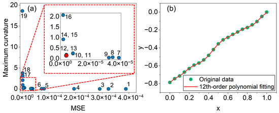
Based on the final sample parameters selected from the optimization algorithm, it is worth noting that the parameter combinations generated by the algorithm inherently contain random fluctuations. Although the overall blade morphology has been highly evaluated within the surrogate model, these local random variations can produce singular curvature features on the blade, potentially compromising manufacturability and aerodynamic performance. To mitigate this issue, the present study applies polynomial interpolation to fit and smooth the optimized blade morphology parameters (c1~c20), thereby enhancing the engineering applicability of the resulting blade centerline. Figure 19a shows the relationship between the mean squared error (MSE) of the fitted blade centerline (relative to the original data) and the maximum curvature of the fitted result for polynomial degrees 1 to 19. The results indicate that when the polynomial degree is between 7 and 16, both the error and curvature remain at relatively low levels. A 12th-degree polynomial was selected for fitting, as it effectively controls the error while suppressing sharp curvature changes. The mathematical form of the optimized centerline is provided below, along with the final coefficients for the 12th-degree polynomial, rounded to four significant digits.
As shown in Figure 21b, the 12th-order fitted curve aligns well with the original data, with minimal fitting error and a smooth overall contour, free from local fluctuations, thus meeting the blade design requirements for smoothness and precision.
Figure 21.
Polynomial fitting results for 20-dimensional blade morphology parameters after optimization: (a) Relationship between MSE, maximum curvature, and polynomial degree (1–19). (b) Comparison between 12th-order polynomial fitting and original data.
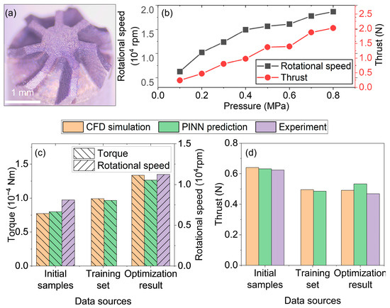
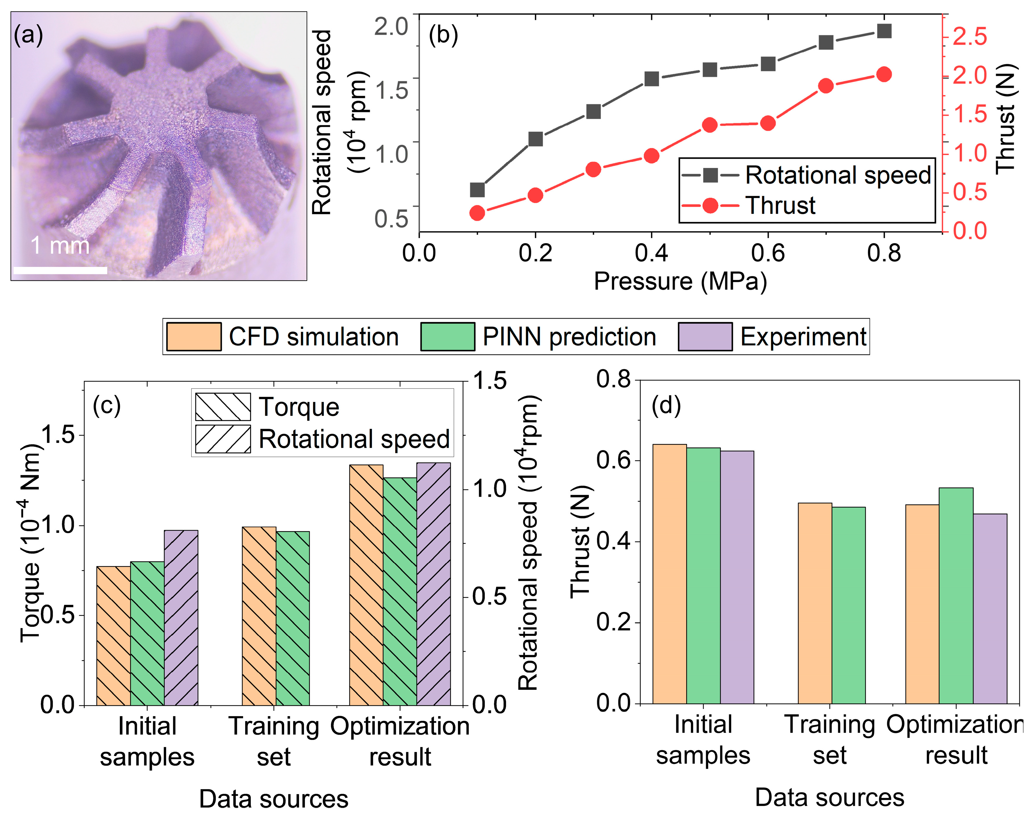
Based on the final optimized blade parameter combination obtained from the above study, the corresponding micro-turbine structure was fabricated and tested, confirming its performance improvement compared with the initial samples. Figure 22 demonstrates the optimized micro-turbine rotor sample and its performance evaluation results. Figure 22a shows a microscopic image of the optimized turbine, featuring 7 blades and displaying good structural integrity. Figure 22b compares the rotational speed and thrust of the optimized turbine with the inlet pressure (0~0.8 MPa). It can be seen that the performance trends of the optimized turbine are generally consistent with those of the initial samples shown in Figure 13, with both the rotational speed and thrust showing a monotonic increase across the entire operational range, confirming that the optimization design has not altered its basic aerodynamic response characteristics. Figure 22c,d compare the performance differences at various design stages in terms of torque and thrust. From the data obtained through CFD simulation and PINN model prediction, the model’s prediction error is relatively small for the initial and training set samples. For the optimized samples, although the prediction error slightly increases, it remains within 10%, indicating that the established PINN model possesses good generalization and extrapolation ability. Figure 22c shows that, after sample expansion and active learning, the maximum torque of the training set samples has increased compared to the initial samples. Moreover, after the multi-objective optimization with the NSGA-II algorithm, the torque performance of the optimal sample has been significantly enhanced, demonstrating the effectiveness of the parametric design and intelligent optimization approach. It is important to note that, for thrust, some training set samples experience a decrease in thrust as torque increases. However, the optimized sample does not exhibit any further decrease in thrust, indicating that the optimization process has effectively minimized thrust degradation while significantly enhancing torque.
Figure 22.
Optimization and performance evaluation of the micro-turbine: (a) Optimized micro-turbine. (b) Turbine rotational speed and thrust performance at different pressures. (c) Comparison of torque performance before and after optimization. (d) Comparison of thrust performance before and after optimization.
Under the typical operating condition of 0.2 MPa inlet pressure, the optimized sample achieves a 38.6% increase in rotational speed compared with the initial optimal sample, while maintaining 75.1% of the original thrust. This demonstrates the potential of this optimization strategy in improving the turbine’s dynamic response and energy conversion efficiency. This performance trade-off aligns well with the core requirements of compact reconnaissance and low-speed long-endurance MAVs, where the gains in shaft power density and energy efficiency from the elevated rotational speed far outweigh the impact of moderate thrust reduction, and the retained thrust is fully adequate for stable low-speed flight and hovering.
4. Conclusions
This study presents an integrated framework for the intelligent design of 3 mm micro-turbine blades, combining fabrication-aware parametric modeling, a PINN surrogate, and a two-stage active learning strategy, with validation through micro-fabrication and aerodynamic testing. To balance high-dimensional design freedom with micro-EDM manufacturability, the three-dimensional blade surface is parameterized as a centerline sequence controlled by 22 variables, ensuring both geometric accessibility and sufficient flexibility for aerodynamic optimization. To address the high computational cost and limited generalization of traditional surrogate models, a PINN-based flow prediction model is constructed, and a two-stage active learning approach integrating KD-tree spatial exploration and residual-based adaptive sampling is employed. Starting from only 10 initial samples, a high-accuracy surrogate with 500 samples is obtained, significantly improving prediction and generalization in the 22-dimensional design space. Using this surrogate, multi-objective optimization via NSGA-II identifies a Pareto-optimal set for torque and thrust, revealing the trade-offs between performance objectives. The optimized blade, smoothed with a 12th-degree polynomial, is fabricated and tested, achieving a 38.6% increase in rotational speed while retaining 75.1% of thrust at 0.2 MPa inlet pressure, demonstrating both performance enhancement and manufacturability. In summary, this work establishes a systematic methodology from parametric modeling and intelligent surrogate construction to automated multi-objective optimization and experimental verification, providing a reliable framework for the design of high-dimensional, fabrication-constrained microfluidic devices.
Author Contributions
Conceptualization, Y.H., L.Z., S.G. and Z.W.; Data curation, Y.H. and S.G.; Formal analysis, Y.H. and L.Z.; Funding acquisition, Z.W.; Investigation, Y.H. and L.Z.; Methodology, Y.H., L.Z., S.G. and Z.W.; Project administration, Z.W.; Resources, Z.W.; Software, Y.H.; Supervision, Z.W.; Validation, Y.H., L.Z. and S.G.; Visualization, Y.H.; Writing—original draft, Y.H. and L.Z.; Writing—review and editing, S.G. All authors have read and agreed to the published version of the manuscript.
Funding
This work is supported by the National Natural Science Foundation of China (Grant No. 52175390).
Institutional Review Board Statement
Not applicable.
Informed Consent Statement
Not applicable.
Data Availability Statement
The original contributions presented in this study are included in the article. Further inquiries can be directed to the corresponding author.
Conflicts of Interest
The authors declare no conflicts of interest.
Abbreviations
The following abbreviations are used in this manuscript:
| CFD | Computational Fluid Dynamics |
| EDM | Electrical Discharge Machining |
| GAN | Generative Adversarial Network |
| LHS | Latin Hypercube Sampling |
| LSTM | Long Short-Term Memory |
| MAV | Micro Aerial Vehicle |
| MSE | Mean Squared Error |
| NSGA-II | Non-dominated Sorting Genetic Algorithm II |
| PINN | Physics-Informed Neural Network |
| PTFE | Polytetrafluoroethylene |
| RANS | Reynolds-Averaged Navier–Stokes |
References
- Chopra, I. Small UAS and delivery drones: Challenges and opportunities the 38th Alexander A. Nikolsky honorary lecture. J. Am. Helicopter Soc. 2021, 66, 1–41. [Google Scholar] [CrossRef] [Scilit]
- Ju, Y.; Maruta, K. Microscale combustion: Technology development and fundamental research. Prog. Energy Combust. Sci. 2011, 37, 669–715. [Google Scholar] [CrossRef] [Scilit]
- Epstein, A.H.; Senturia, S.D. Microengineering—Macro power from micro machinery. Science 1997, 276, 1211. [Google Scholar] [CrossRef] [Scilit]
- Kang, S.; Johnston, J.P.; Arima, T.; Matsunaga, M.; Tsuru, H.; Printz, F.B. Microscale radial-flow compressor impeller made of silicon nitride: Manufacturing and performance. J. Eng. Gas Turbines Power 2004, 126, 358–365. [Google Scholar] [CrossRef] [Scilit]
- Cooper, A.G.; Kang, S.; Kietzman, J.W.; Prinz, F.B.; Lombardi, J.L.; Weiss, L.E. Automated fabrication of complex molded parts using mold shape deposition manufacturing. Mater. Des. 1999, 20, 83–89. [Google Scholar] [CrossRef] [Scilit]
- Cooper, A.G.; Kang, S.; Kietzman, J.W.; Prinz, F.B.; Lombardi, J.L.; Weiss, L. Automated Fabrication of Complex Molded Parts Using Mold SDM. In Proceedings of the 9th Solid Freeform Fabrication (SFF) Symposium, Austin, TX, USA, 10–12 August 1998. [Google Scholar]
- Yoshida, J.; Matsuo, E.; Takata, Y.; Monde, M. Thermodynamic analysis of high pressure hydrogen gas refueling system with turbo-expanders. Mech. Eng. J. 2019, 6, 18-00388. [Google Scholar] [CrossRef] [Scilit]
- Isomura, K.; Tanaka, S.; Togo, S.; Kanebako, H.; Murayama, M.; Saji, N.; Sato, F.; Esashi, M. Development of micromachine gas turbine for portable power generation. JSME Int. J. Ser. B Fluids Therm. Eng. 2004, 47, 459–464. [Google Scholar] [CrossRef] [Scilit]
- Isomura, K.; Togo, S.-i.; Hikichi, K.; Goto, S.; Tanaka, S. Analytical and Experimental Study of Hydroinertia Gas Bearings for Micromachine Gas Turbines. In Proceedings of the 50th ASME Turbo-Expo, Reno, NV, USA, 6–9 June 2005. [Google Scholar]
- Hikichi, K.; Goto, S.; Togo, S.; Tanaka, S.; Isomura, K. Hydroinertia gas bearings for micro spinners. J. Micromech. Microeng. 2005, 15, S228–S232. [Google Scholar] [CrossRef] [Scilit]
- Isomura, K.; Tanaka, S.; Togo, S.; Esashi, M. Development of high-speed micro-gas bearings for three-dimensional micro-turbo machines. J. Micromech. Microeng. 2005, 15, S222–S227. [Google Scholar] [CrossRef] [Scilit]
- Peirs, J.; Reynaerts, D.; Verplaetsen, F. A microturbine for electric power generation. Sens. Actuators A Phys. 2004, 113, 86–93. [Google Scholar] [CrossRef] [Scilit]
- Keding, M.; Dudzinski, P.; Reissner, A.; Hummel, S.; Tajmar, M. Improved μ-Scale Turbine Expander for Energy Recovery. In Proceedings of the ASME Turbo Expo 2010, Glasgow, UK, 14–18 June 2010. [Google Scholar]
- Waitz, I.A.; Gauba, G.; Tzeng, Y.S. Combustors for micro-gas turbine engines. J. Fluids Eng. 1998, 120, 109–117. [Google Scholar] [CrossRef] [Scilit]
- Shan, X.C.; Zhang, Q.D.; Sun, Y.F.; Wang, Z.F. Design, Fabrication and Characterization of an Air-Driven Micro Turbine Device. In Proceedings of the International MEMS Conference 2006, Singapore, 9–12 May 2006. [Google Scholar]
- Fu, L.; Feng, Z.P.; Li, G.J. Experimental investigation on overall performance of a millimeter-scale radial turbine for micro gas turbine. Energy 2017, 134, 1–9. [Google Scholar] [CrossRef] [Scilit]
- Fu, L.; Feng, Z.P.; Li, G.J. Investigation on design flow of a millimeter-scale radial turbine for micro gas turbine. Microsyst. Technol. 2018, 24, 2333–2347. [Google Scholar] [CrossRef] [Scilit]
- Shao, S.; Deng, Q.H.; Feng, Z.P. Aerodynamic Optimization of The Radial Inflow Turbine for a 100kw-Class Micro Gas Turbine Based on Metamodel-Semi-Assisted Method. In Proceedings of the ASME Turbo Expo: Turbine Technical Conference and Exposition, San Antonio, TX, USA, 3–7 June 2013. [Google Scholar]
- Fu, L.; Shi, Y.; Deng, Q.H.; Feng, Z.P. Aerodynamic design and numerical investigation on overall performance of a microradial turbine with millimeter-scale. J. Eng. Gas Turbines Power 2010, 132, 032301. [Google Scholar] [CrossRef] [Scilit]
- Fu, L.; Feng, Z.P.; Li, G.J. Discussions on problem analysis and solutions of a micro turbine test. Microsyst. Technol. 2018, 24, 1433–1442. [Google Scholar] [CrossRef] [Scilit]
- Holmes, A.S.; Hong, G.D.; Pullen, K.R. Axial-flux permanent magnet machines for micropower generation. J. Microelectromech. Syst. 2005, 14, 54–62. [Google Scholar] [CrossRef] [Scilit]
- Farhat, H.; Altarawneh, A. Physics-informed machine learning for intelligent gas turbine digital twins: A review. Energies 2025, 18, 5523. [Google Scholar] [CrossRef] [Scilit]
- Gao, E.N.; Ming, Y.; Zhao, K.W.; Shu, Y.D.; Xu, F.Y. A hybrid fault diagnosis framework for rudder propellers: Physics-guided learning from data and simulation. Ocean Eng. 2026, 351, 124419. [Google Scholar] [CrossRef] [Scilit]
- Li, Y.X.; Liu, W.H.; Sun, C.B.; Cui, M.; Ren, J.W.; Nikolaitchik, M.A. A physics-informed LSTM framework for solving fluid flow and heat transfer coupling problem of the turbine vane as well as the internal cooling optimization. Aerosp. Sci. Technol. 2026, 168, 111300. [Google Scholar] [CrossRef] [Scilit]
- Wang, P.Y.; Pan, B.L.; Liu, Z.; Gao, L.J. FDPI-DeepONet: A novel integration for 3D airfoil flow field computation. Acta Mech. Sin. 2026, 42, 725215. [Google Scholar] [CrossRef] [Scilit]
- Tong, Z.M.; Chen, R.Z. Physics-informed spatiotemporal neural network for unsteady propeller wake prediction via least squares finite-difference framework. Phys. Fluids 2026, 38, 025132. [Google Scholar] [CrossRef] [Scilit]
- Rahman, M.A.; Prantik, M.F.R.; Islam, S.M.T.; Rahman, A.; Masum, S.H.; Hossain, M.A. Hyperdimensional computing and ridge regression for airfoil aerodynamic prediction: A physics-informed machine learning framework. Aerosp. Sci. Technol. 2026, 171, 111591. [Google Scholar] [CrossRef] [Scilit]
- Xiao, Z.Y.; He, B.J.; Zhang, B.Y.; Chen, Y.T.; Cai, G.B.; Weng, H.Y. A physics-informed neural network model for viscous compressible turbulent flows simulations within a rocket engine nozzle. Aerosp. Sci. Technol. 2026, 171, 111598. [Google Scholar] [CrossRef] [Scilit]
- Huang, L.J.; Geng, L.; Li, A.B.; Yang, F.Y.; Peng, H.X. In situ TiBw/Ti-6Al-4V composites with novel reinforcement architecture fabricated by reaction hot pressing. Scr. Mater. 2009, 60, 996–999. [Google Scholar] [CrossRef] [Scilit]



Disclaimer/Publisher’s Note: The statements, opinions and data contained in all publications are solely those of the individual author(s) and contributor(s) and not of MDPI and/or the editor(s). MDPI and/or the editor(s) disclaim responsibility for any injury to people or property resulting from any ideas, methods, instructions or products referred to in the content. |
© 2026 by the authors. Licensee MDPI, Basel, Switzerland. This article is an open access article distributed under the terms and conditions of the Creative Commons Attribution (CC BY) license.